Marginalization using the metric of the likelihood

Given data $\vec{d}$, a linear parameter $c$ and some function $\vec{f}$ meant to explain the data, we have

The vectors shall have dimension $N$ according to the number of quantities measured. Due to the measurement process the data is corrupted by noise, where $\langle\varepsilon\rangle=0$ and $\langle\varepsilon^{2}\rangle=\sigma^{2}$. Then by the principle of Maximum Entropy the likelihood function reads

which is clearly normalizeable for the data $\vec{d}$ and bound for every parameter showing up as a functional dependency in $f$. The situation may change when we are looking for the expectation value of some parameter of $f$, let say $f=f(T)$. Then we need to evaluate the posterior of $T$ with

In order to connect the unknown posterior to the known likelihood we marginalize over all the parameters which enter the problem, that is in our problem $c$ and $\sigma$:

and make use of Bayes theorem:

Commonly, the infinitesimal elements in equation (4) are identified with

In mathematical terms this would mean that the probability functions live in euclidean space. They do not.

Parameterizations correspond to choices of coordinate systems. The problem to be solved has to be invariant against reparametrizations rod89, i.e. in the space of the probability functions one has to get the same answer no matter what parameters were chosen to describe a model. Therefore one is in need of a length measure $\mu$ which takes care of defining a distance between different elements of this probability function space. This task is done by applying differential geometry to statistical models, an approach which was baptized ’information geometry’ by S. Amari ama85. Eq. (6) then reads correctly

$\mu({\rm d}\vec{\theta})=\mu(\vec{\theta}){\rm d}\vec{\theta}$ is the natural Riemannian metric on a regular model (in our case the model is parameterized by $\vec{\theta}=(T,c,\sigma)$). It results from second variations of the entropy ama85; rod91 and is given by

where g is the Fisher information matrix:

For the above likelihood the metric reads explicitly

Notice that this approach is based on the assumption that the hypothesis space of the likelihood defines the metric to be calculated in. This may not be the case if some prior information was already used during data acquisition, e.g. the experimentalist uses his expert knowledge in separating ’correct’ data from the rest. The latter instantly rules out certain parts of all possible realizations of the likelihood function and results in a different hypothesis space.

First we want to demonstrate the relevance of using the correct metric with a simple example which already has all the features of the real world problem further down.

where the notation in $i$ corresponds to the data points $d_{i}$. For simplification let us assume that the variance $\sigma^{2}$ is known and we only have to marginalize over $c$ in order to get the posterior. What happens if we do not use the Riemannian metric? Then the marginalization integral over $c$ reads

In order to facilitate analytic calculation the exponent of the likelihood is written in a quadratic form over $c$

where $c_{0}=\vec{d}^{T}\vec{f}/\vec{f}^{T}\vec{f}$. For the prior $p(c|I)$ the only thing we know is that $c$ will be something in between an upper and a lower limit, where it is reasonable to assume that the upper (lower) bound is given by an unknown factor $n$ (1/$n$) of the value $c_{0}$ where the maximum of the likelihood occurs. The principle of maximum entropy gives a flat prior with

The integral over the c-dependent parts then reads

One may check that for $\vec{f}^{T}\vec{f}\gg\sigma^{2}$ it is allowed to shift the integral boundaries to $+/-$ infinity with affecting the value of the integrand up to a small error only. As a matter of fact for the chosen model parameters of $N$=3, $x_{i}$=$i$, $T$=1, c=1 and $\sigma$=0.1 the error is in the order of $10^{-7}$ of the correct integral. Notice that this is almost the same for every $T$ in between 0 and infinity. We finally get

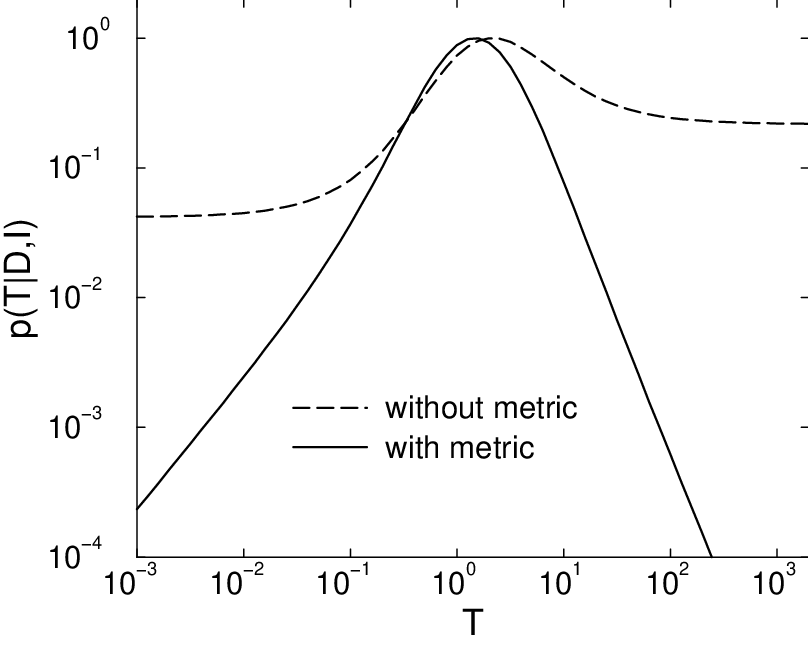
A look at the behavior for large and small T gives

Though one has no problem with the lower limit since the integrand is regular, the non-vanishing posterior distribution for $T\rightarrow\infty$ leads to an expectation value which depends on where the integration limits are set (see Fig. 1).

Now we implement in the calculation the Riemannian metric. From Eq. (10) we get an additional factor $c$, so the integration over the $c$-dependent parts changes to

Again it is allowed to extend the integration limits to $+/-$ infinity with only minor error. The full posterior then gives

What is now the behavior of $p(T|D,I)$ for $T$ approaching 0 and infinity? The exponent in Eq. (20) was already examined in Eqn. (17) and (18) to become constant, so we only have to look at the square root.

So indeed the square root term which stems from the metric does take care of zero tails in the posterior! The nice decrease towards 0 is shown in Fig. 1 by the solid line.

In the problem of determining the electron temperature in an hydrogen plasma heated by electron cyclotron resonance, the model function $T$ depends in a quite complicated way on the temperature $T$:

Both V and R are matrices, but only the diagonal matrix V depends on T with entries on the diagonal:

where $a_{i}$ and $b_{i}$ are constants with respect to ion species $i$. Since the sensitivity of the measurement apparatus is unknown one has to introduce a linear parameter $c$ in order to relate the data to the model, i.e. Eq. (1). Contrary to our simple problem we are not so fortunate to know the variance $\sigma$ exactly. The experimentalist can only provide an estimate $\vec{s}$ of the true errors $\vec{\sigma}$ with respect to each other but not on the total scale, so that we have to introduce an overall multiplication factor $\omega$, with $\sigma_{i}=\omega s_{i}$. In order to assign a prior to $\omega$ the outlier tolerant approach dol99 was chosen:

The expectation value of $\omega$ should be one, since the experimentalist does his estimation according to his best knowledge. Furthermore, from the characteristics of the measurement process one can tell that the best guess of $\vec{s}$ should not deviate by more than 50% from the true $\vec{\sigma}$. This results in $\alpha=1.28$ and $\gamma=2.0076$.

Now we follow the route explained above to evaluate the expectation value of $T$. Again we start by marginalizing $c$ (with the flat prior of Eq. (14)) and $\omega$ without making use of the Riemannian metric. This gives the posterior in $T$

For simplicity of notation the hat shall denote that the values have been divided by the estimated error $\vec{s}$: $\hat{d}_{i}=d_{i}/s_{i}$. The posterior is displayed in Fig. 2. Here we have to face the problem we observed above in the simple example. Though a non-vanishing tail for $T\rightarrow 0$ is not so harmful, the increase with $T\rightarrow\infty$ results in a divergence.

Help comes by obeying the correct Riemannian metric. Then the posterior reads

where $\mu(T)$ is just the metric of Eq. (10) without the terms in $c$ and $\omega$ (marginalized over). The situation changes completely (see Fig. 2) and the integral becomes feasible now.

The correct mathematical way to deal with marginalization integrals is to use the Riemannian metric. This invariant measure takes care of defining correct infinitesimal elements to be integrated over. Since parameterizations of a model may be subjective and vary with the investigator of a problem, this is the only consistent way to get comparable answers in probability space.

We like to acknowledge discussions with C. Rodriguez.

References

- (1) C. Rodriguez, “The metrics induce by the kullback number,” in Maximum Entropy and Bayesian Methods, J. Skilling, ed., Kluwer Academic, Dordrecht, 1989.
- (2) S. Amari, Differential-Geometrical Methods in Statistics, Springer-Verlag, Berlin, Heidelberg, 1985.
- (3) C. Rodriguez, “From euclid to entropy,” in Maximum Entropy and Bayesian Methods, J. W. T. Grandy, ed., Kluwer Academic, Dordrecht, 1991.
- (4) V. Dose and W. von der Linden, “Outlier tolerant parameter estimation,” in Maximum Entropy and Bayesian Methods, V. Dose et al., ed., Kluwer Academic, Dordrecht, 1999.