Transient behavior in Single-File Systems
Abstract
We have used Monte-Carlo methods and analytical techniques to investigate the influence of the characteristics, such as pipe length, diffusion, adsorption, desorption and reaction rates on the transient properties of Single-File Systems. The transient or the relaxation regime is the period in which the system is evolving to equilibrium. We have studied the system when all the sites are reactive and when only some of them are reactive. Comparisons between Mean-Field predictions, Cluster Approximation predictions, and Monte Carlo simulations for the relaxation time of the system are shown. We outline the cases where Mean-Field analysis gives good results compared to Dynamic Monte-Carlo results. For some specific cases we can analytically derive the relaxation time. Occupancy profiles for different distribution of the sites both for Mean-Field and simulations are compared. Different results for slow and fast reaction systems and different distribution of reactive sites are discussed.
pacs
02.70.Uu, 02.60.-x, 05.50.+q, 07.05.TpI Introduction
Although systems in nature evolve by obeying physical laws, it is in most cases difficult or not feasible to describe the system properties accurately since details of the microscopic dynamics are not fully known. Therefore we usually deal with simplified models for these systems of which stochastic models are an example. They are thus described by a reduced set of dynamic variables. Although many exact solutions have been found, Baxter 1982; Derrida and Evans 1997; Alcaraz 1994; Derrida et al. 1992; Schutz and Domany 1993; Derrida et al. 1993 the vast majority of stochastic models cannot be solved exactly. Many results for equilibrium systems J.G.Tsikoyannis and Wei 1991; R ¨ o denbeck et al. 1997; Okino et al. 1999; Coppens et al. 1998; Coppens et al. 1999 have been classified. In nature, however, equilibrium is rather an exception than a rule. In most cases the temporal evolution starts from an initial state which is far away from equilibrium. The relaxation of such a system towards its stationary state depends on the specific dynamical properties and cannot be described within the framework of equilibrium statistical mechanics. Instead it is necessary to set up a model for the microscopic dynamics of the system. Assuming certain transition probabilities, the time-dependent probability distribution to find the system in configuration has to be derived from the Master Equation (ME). Solving the ME is usually a difficult task. Therefore, the theoretical understanding of non-equilibrium processes is still at its beginning. Better understanding of these phenomena would be an important step as non-equilibrium systems exhibit a richer behavior than equilibrium systems. Privman 1997; Marro and Dickman 1998; Dickman and Jensen 1991; Grinstein et al. 1989; Dickman and Burschka 1988
We investigate non-equilibrium processes for a Single-File System (SFS) with conversion. In S.V.Nedea et al. 2002 we have already elaborated on the special properties of porous structures such as zeolites. The one-dimensional nature of the zeolite channel leads to extraordinary effects on the kinetic properties of these materials. These structures are modelled by one-dimensional systems called Single-File Systems where particles are not able to pass each other. In S.V.Nedea et al. 2002 we have focused on the steady-state properties of a SFS with conversion. The process of diffusion in SFS has different characteristics as ordinary diffusion, which affects the nature of both transport and conversion by chemical reactions. We are investigating the kinetic properties of this system, and, more precisely, we are interested in the properties of the system before reaching equilibrium (the transient or relaxation regime).
Different methods and techniques have been described in the literature to solve the ME exactly. R ¨ o denbeck et al. 1997; Privman 1997; Derrida and Evans 1999 In spite of the remarkable progress in the field of exactly solvable non-equilibrium processes, the majority of reaction-diffusion models cannot be solved exactly. Ben-Naim and Krapivsky 1994; Derrida et al. 1996 It is therefore necessary to use approximation techniques in order to describe their essential properties (e.g. Mean-Field Approximation, Cluster Approximation). J.Mai et al. 1994a Also, as was already realized by Smoluchowski, von Smoluchowski 1917 fluctuations and correlations may be extremely important in low-dimensional systems where the diffusive mixing is not strong. Therefore, these approximation techniques can give results that deviate strongly from the system behavior. Dynamic Monte Carlo methods are used to simulate the system according to the ME.
Few researchers have concentrated on the properties of the system in the transient regime and only studied the reactivity of the system in this regime. Moreover, few research has been done for an open system where adsorption/desorption is present at the marginal sites. The reason that many of the analytical approaches fail is because of the asymmetry of the system.
In the present work we focus on the non-equilibrium phase properties of SFS with conversion. We study the relaxation time of the system (time evolution of the system properties, starting with no particles) for different sets of kinetic parameters, lengths of the pipe and distributions of the reactive sites. In the transient regime we observe that MF results are close to the DMC results both for slow and fast reaction systems. We outline the cases for which the differences are significant. We compare with the steady-state situation in which the MF was not describing the Single-File effects properly. S.V.Nedea et al. 2002 We analyze the situations when analytical results can be derived, and we compare these results with Mean-Field (MF) and Dynamic Monte Carlo (DMC) results. We look at the relaxation of the total loading, loading with different components, occupancies of individual sites for various parameters and different distributions of the reactive sites. As MF is a coarse approximation, for the analysis of profile occupancies we introduce a better approximation (Cluster Approximation). We analyse the results using different analytic methods such as pair and MF approximation. Pair Approximation and MF Approximation tend to give similar results due to the high-order correlations in the system. We investigate the effect of various model assumptions made about diffusion, adsorption, desorption and reaction on the kinetic behavior of the system.
In section II we specify our mathematical model together with the theoretical background for analytical and simulation results. In section III.1 we present the various results for transient regimes for the simplified model without conversion. We solve numerically and analytically the Master Equation in order to get the relaxation time of the system. In section III.2 we use MF theory to simplify the rate equations S.V.Nedea et al. 2002 of the system for the case when all the sites have the same activity towards conversion. We present the results obtained using DMC simulations for the case with conversion when all the sites are reactive in section III.3.1, and when only some of the sites are reactive in section III.3.2. For all of these cases we compare the DMC results with MF and Pair Approximation results. The influence of the position of the reactive sites is also outlined. The last section summarizes our main conclusions.
II Theory
In this section we give the theoretical background for our analytical and simulation results. First we specify our model and then we show that the defined system obeys a Master Equation (ME). We derive then a set of exact rate equations from the Master Equation of the system describing the reaction kinetics. We look at the properties of the system in the transient regime by solving these rate equations. In order to do this we have to use approximation techniques. We use MF analysis and we derive a set of equations that we can solve numerically. Because MF is a strong simplification and neglects all spatial correlations in the system, we introduce another approximation called the Cluster Approximation. We have also simulated the system governed by the ME using DMC simulations.
II.1 The Model
We model a Single-File System by a one-dimensional array of sites, each possibly occupied by an adsorbate. This is the model of diffusion and reaction in a one-dimensional arrangements of particles with hard-core interaction. The sites are numbered . A particle can only move to the right or to the left if an adjacent site is vacant. The sites could be reactive and unreactive and we note with the number of reactive sites. A reactive site is the only place where a conversion may take place.

We consider two types of adsorbates, and , in our model and we denote
with the site occupation of a site, =(, , ), which stands for a
vacant site, a site occupied by , or a site occupied by a , respectively.
We restrict ourselves to the following mono- and bi-molecular transitions.
a) Adsorption and desorption
Adsorption and desorption take place only at the two marginal sites
i.e., the left and rightmost sites at the ends of the system.
+
+
+
where subscripts denotes a marginal site. Note that there is no adsorption.
’s can only be formed by conversion.
b) Diffusion
In the pipe, particles are allowed to diffuse via hopping to
vacant nearest neighbor sites.
+ +
+ +
where the subscripts are site indices: = 1, 2, , -1.
c) Conversion
An can transform into a at a reactive site.
.
In the initial state of the system all the sites are vacant (no particles in the pipe) as we are interested in the behavior of the system towards equilibrium.
II.2 Master Equation
Reaction kinetics is described by a stochastic process. Every reaction has a microscopic rate constant associated with it that is the probability per unit time that the reaction occurs. Stochastic models of physical systems can be described by a Master Equation. Kampen 1981
By , , we will indicate a particular configuration of the system i.e., a particular way to distribute adsorbates over all the sites. will indicate the probability of finding the system in configuration at time and is the rate constant of the reaction changing configuration to configuration .
The probability of the system being in configuration at time can be expressed as the sum of two terms. The first term is the probability to find the system already in configuration at time multiplied by the probability to stay in this configuration during . The second term is the probability to find the system in some other configuration at time multiplied by the probability to go from to during .
| (1) |
By taking the limit this equation reduces to a Master Equation:
| (2) |
Analytical results can be derived as follows. The value of a property is a weighted average over the values which is the value of in configuration :
| (3) |
From this follows the rate equation
| (4) |
II.3 Analytical methods
II.3.1 Rate equations
Starting from the Master Equation (2) and using expression (4) the rate equations of the system are derived. S.V.Nedea et al. 2002 We denote by , , the rate constants of adsorption, desorption and diffusion respectively. For simplicity we assume that the rate constants of and desorption are equal, and also the rate constants of and diffusion are equal. We denote by the probability that a particle of type is on site , and with the probability that a particle of type is at site and one at site , where =(,,). The coefficients , where =1, 2,, , are 1 if site is reactive and 0 otherwise. The rate equations for a non-marginal site are
| (5) |
For we get similarly
| (6) |
The marginal sites also have adsorption and desorption. They can be dealt with similary as the conversion. The rate equations for are
| (7) |
and the rate equations for
| (8) |
Note that these coupled sets of differential equations are exact, but not closed.
II.3.2 Mean-Field
To solve this coupled set of differential equations, we need to make an approximation for the two-site probabilities such as ,, etc. The closure relation
| (9) |
should hold for any approximation for these two-site probabilities. We denote with the occupation of site and with the occupation of site . The simplest approximation is
| (10) |
i.e. neighboring sites are considered independent.
The two-site probabilities then become =, =. J.Mai et al. 1994a This approximation is called the Mean-Field Approximation and gives us a coupled set of differential equations that we can solve numerically.
II.3.3 Cluster Approximation
The MF Approximation is a strong simplification because it neglects all spatial correlations in the system. Because the system we analyze is one-dimensional, the correlations might be significant and important. The obvious possibility to eliminate the weakness of the MF approach is to introduce another approximation.
Instead of using MF Approximation for the two-site probabilities, we write down their rate equations (see appendix). These equations have three-site probabilities which we approximate. This leads to a so-called Cluster Approximation. The closure relation
| (11) |
should now hold for any approximation. We denote here with the occupation of site , with the occupation of site , and with the occupation of site .
There are various decoupling scheme used in the literature Derrida and Evans 1999; Derrida and Evans 1997; Mamada and Takano 1968; Derrida et al. 1992; Derrida et al. 1993 as approximations for the -site probabilities. For many of these decoupling schemes the closure relation (11) no longer holds. For simplicity we will use the simplest Cluster Approximation, called Pair Approximation for which only the correlations between pairs of nearest neighbors (NN) are considered.
The decoupling scheme for our pair Approximation is
| (12) |
It is straightforward to see that the closure relation (11) holds.
| (13) |
After decoupling, this system of coupled sets of differential equations, consisting of the rate equations for one-site and two-site probabilities, becomes closed and can be solved numerically.
II.4 Dynamic Monte Carlo
We have seen that we can derive approximate analytical solutions to the Master Equation. DMC methods allow us to simulate the system governed by the Master Equation over time. We simplify the notation of the Master Equation by defining a matrix containing the rate constants , and a diagonal matrix by , if , and 0 otherwise. If we put the probabilities of the configurations in a vector , we can write the Master Equation as
| (14) |
where and are time independent. We also introduce a new matrix , This matrix is time dependent by definition and we can rewrite the Master Equation in the integral form
| (15) |
By substitution we get from the right-hand-side for
| (16) |
Suppose at the system is in configuration with probability . The probability that, at time , the system is still in configuration is given by . This shows that the first term represents the contribution to the probabilities when no reaction takes place up to time . The matrix determines how the probabilities change when a reaction takes place. The second term represents the contribution to the probabilities when no reaction takes place between times and , some reaction takes place at time , and then no reaction takes place between and . The subsequent terms represent contributions when two, three, four, etc. reactions take place. The idea of the DMC method is not to compute probabilities explicitly, but to start with some particular configuration, representative for the initial state of the experiment one wants to simulate, and then generate a sequence of other configurations with the correct probability. The method generates a time when the first reaction occurs according to the probability distribution . At time a reaction takes place such that a new configuration is generated by picking it out of all possible new configurations with a probability proportional to . At this point we can proceed by repeating the previous steps, drawing again a time for a new reaction and a new configuration. Lukkien et al. 1998; R.J.Gelten et al. 1998a
III Results and Discussion
In S.V.Nedea et al. 2002 various results for the system with conversion () and without conversion() were reported. In case we have only particles in the system. The total loading () of the system is defined as the average number of particles per site. In case we have ’s as well in the system. In this case, the total loading (), is the sum of the loading with particles () and loading with particles ()
| (17) |
Note that the total loading of the pipe for the model with conversion is the same as for the model without conversion. S.V.Nedea et al. 2002 We study the relaxation time of the system without conversion and of the system with conversion.
III.1 No conversion
We are interested in the relaxation time of the system (transients). We start with the evolution of the total loading over time starting from a system with no particles at all. As the total loading is the same for the case with and without conversion, we will consider for simplicity the case with no conversion first.
As we can derive a finite set of exact rate equations(5,6,7,8) it’s not necessary to work with the Master Equation in this case. With the probability that site is occupied we have
| (18) |
when is not a marginal site. The two-site probabilities can be eliminated by using closure relations,
| (19) |
that hold in this specific case. The probabilities with particles on both neighboring sites cancel and the result is
| (20) |
For the marginal sites we get
| (21) |
These equations are used for the derivation of the relaxation time. The rate equations are going to be simplified to a point where they are a set of homogeneous linear ODE’s with only one parameter apart from the system size. Dividing by and introducing the dimensionless parameters
| (22) |
we get
| (23) |
We can write these equations in matrix-vector notation as
| (24) |
where is a vector containing the occupancy probabilities, is the matrix of coefficients having the form
| (25) |
and is the vector that makes the system non-homogeneous. The parameter is the equilibrium coverage.
Finally we can make the set of equations homogeneous by working with probabilities for vacancies: i.e., with
| (26) |
we get
| (27) |
In order to solve equation (27), we try the substitution
| (28) |
Taking out the exponential leaves us with
| (29) |
Removing the time dependence yields relaxation times. We see that we have obtained an eigenvalue equation. The eigenvalues are the reciprocal of relaxation times for the corresponding eigenvectors. The relaxation time of the system as a whole() is the reciprocal of the smallest eigenvalue. We can get this time by simply numerically solving the eigenvalue equation for given and .
Solving the eigenvalue equation analytically.
For some special cases analytical expressions for the eigenvalues can be given. We consider the ansatz
| (30) |
If we substitute from expression (29) into the equation for not a marginal site, we get
| (31) |
This equation has two solutions.
| (32) |
where
| (33) |
There are two cases to be distinguished. If then both solutions are real. Because this is the same as , we will have this for slow diffusion and for eigenvectors with fast relaxation (large ). As we are interested in the slowest relaxation (small ) we will look at the other case or . The two solutions are then each others complex conjugate. (Note for the following that .)
Fast diffusion or slow relaxation.
In this case we can write the solutions as
| (34) |
where and are both real. In fact the equation for shows that when is a solution, then so is . This means that , or
| (35) |
Substitution in the equation for yields
| (36) |
This has indeed only solutions for .
Because there are two solutions for , the solution for is a linear combination of these two solutions: i.e.,
| (37) |
From equation (28) we remark that should be always real. This means that is the complex conjugate of . The coefficients will follow from the equations for the marginal sites. There are two of these equations. The equation above for is a third equation. We have four unknowns (, , , and ), but, as only the ratio between the coefficients can be determined, we should effectively be able to determine all of them.
Substitution of the expression for in the equations for the marginal sites taking into account that and are complex conjugate (), leads to
| (38) |
This equation only has non-trivial solutions (the trivial solution is ) when the determinant of the matrix equals zero. This leads to the following equation
| (39) |
We can eliminate using .
Using as parameter in equation (39), , we can get the ’s. Equations (35) and (32) gives us the ’s. We get in this way as a function of , coupled by the parameter (see figure 2c).
Solving the eigenvalue equation for the total loading, in the case
We solve the eigenvalue equation numerically in order to get the relaxation time of a system. We want to describe how the relaxation time of the total loading () depends on system parameters like reaction, adsorption/desorption, diffusion rate constants and system size . In figure 2 we show the influence of diffusion on the relaxation time for a system of size =30. Note that there are two regimes describing the dependence on diffusion of the relaxation time . The first regime is for slow diffusion, when decreases rapidly with increasing diffusion, and the second for fast diffusion, when slowly decreases with diffusion to a limiting value.

Because diffusion is infinitely-fast all the sites have the same probability to be occupied and the system is homogeneous. We can then analytically derive the limiting value of for infinitely-fast diffusion from the equation
| (40) |
The first term is the probability of a particle to be adsorbed at the two open ends, and the second is the probability of a particle to be desorbed at the two open ends. The probability of a particle to be adsorbed to one end equals the adsorption rate constant () times the probability to have there a vacancy (1-), while the probability of a particle to be desorbed equals the desorption rate constant () times the probability to have a particle ().
From the above equation we get the expression for ,
| (41) |
The relaxation time is
| (42) |
This limiting value is the same as the one indicated by the convergence of the curves in figure 2. The other parameter that influence the relaxation time is the length of the pipe . For diffusion very fast, increases linearly with (see figure 3).

III.2 Conversion
In the case with no conversion, we have derived a set of exact equations and we have simplified the rate equations to homogeneous linear ODE’s. Including conversion in our model, the two-site probabilities can not be eliminated and an approximation is needed. We use the MF Approximation and we get a coupled set of differential equations that we can solve numerically. In figure 4, from the MF results for the transients, we observe that there are two different behaviors determined by conversion.
For fast reaction systems (see figure 4a), the relaxation time of the loading with ’s () and ’s () is equal to the relaxation time of the total loading (). This means that when has reached equilibrium, and have also reached equilibrium.
For slow reaction systems (see figure 4b), the total loading relaxes faster to equilibrium than the loading with ’s () and ’s (). The regime between reaching equilibrium and and reaching equilibrium we call the reaction limited regime.


We remark that for slow reaction systems in the reaction limited regime, the vacancy probability can be replaced with the steady-state expression = . The set of equations for the case when all the sites are reactive then becomes
| (43) |
We can use these approximate MF equations for the problem of relaxation of and loadings for the case when the total loading has already reached steady-state. The equations for ’s can be written as
| (44) |
where is a vector containing the occupacy probabilities with ’s, is the matrix of coefficients and is the vector that makes this systems non-homogeneous having the non-zero elements for indices 1 and . We substitute = + in the rate equations (47), where is the vector with the deviations of the site occupancy probabilities with ’s from the steady-state. The substitution yields
| (45) |
because by definition.
The equations in are homogeneous and the matrix of coefficients is the same as the one in the original rate equations. We can obtain the eigenvalue equation by making the substitution
| (46) |
and taking out the exponential from the equations. The relaxation time of the loading() is then the reciprocal of the smallest eigenvalue. We can get this time by simply numerically solving the eigenvalue equation.


Solving the eigenvalue equation for the case with conversion
For fast reaction systems we have seen that using MF, the and loadings have the same relaxation, which is the relaxation of the total loading (see figure 4a). The relaxation of can be thus derived from exact equations (13,14). For slow reaction systems we can derive analytically the relaxation of and for the reaction limited regime. In this case we expect the relaxation of and to be determined only by reaction. From the MF results we remark that desorption has also a strong influence on the transients (see figure 4c). This is happening because, in the case desorption is very high, the adsorbed particles at the marginal sites will hardly diffuse into the pipe, most of them being desorbed immediately. As a result, few particles will succeed in getting to the middle sites and the residence time of the particles near the marginal sites will decrease. The loading of the pipe with particles will converge than slower to steady-state. In figure 5 we can see that the analytical results for the transients obtained solving the eigenvalue equation corresponds to the numerical results obtained using the MF Approximation for the case all the sites are reactive. In figure 6 we have analytical results from the eigenvalue equation and MF results for the system in reaction limited regime and for different distributions of the reactive sites. We observe that for marginal sites reactive the results are similar but differ considerably for the middle sites reactive and for the homogeneous distribution of the reactive sites.


Analytically, solving the eigenvalue equation for a very slow reaction system, we find that the relaxation of () as a function of desorption varies with reaction for low desorption rates and converges to a limiting value for very high rates of desorption (see figure 7-a,b).

The dependence of loading on has two regimes, the first for low desorption rates when loading strongly decreases with desorption, and the second when the loading is converging to a limiting value and the adsorption process takes over the system behavior.
We remark that the analytical results for obtained from the eigenvalue equation don’t give the MF peak of ’s particles accumulated in the transient regime for a slow reaction system.
III.3 Comparisons with simulation results
We present now the results obtained for the transients using DMC methods for different sets of parameters. We compare them with the Mean-Field and Pair Approximation results. As for very large pipes the computational effort is considerable, we study a system of size . We have considered separately the sets of parameters in Table 1.
The sets of parameters from a) to e) are for the cases of low loading and from f) to j) for high loading. The parameters in the table describe the following situations: a) and f) for very slow reaction and slow diffusion; b) and g) for slow reaction and slow diffusion; c) and h) for slow reaction and fast diffusion; d) and i) for fast reaction and slow diffusion; e) and j) for fast reaction and fast diffusion.
As the MF results for the total loading are exact, there are, as expected,
no differences between these results and those of the simulation for the
total loading.
We compare the MF results with the simulation results for the case with
conversion in the case all sites are reactive and when only some of the sites
reactive.
| case | ||||
|---|---|---|---|---|
| a) | 0.2 | 0.8 | 0.05 | 0.01 |
| b) | 0.2 | 0.8 | 0.05 | 0.1 |
| c) | 0.2 | 0.8 | 2 | 0.1 |
| d) | 0.2 | 0.8 | 1 | 2 |
| e) | 0.2 | 0.8 | 10 | 2 |
| f) | 0.8 | 0.2 | 0.05 | 0.01 |
| g) | 0.8 | 0.2 | 0.05 | 0.1 |
| h) | 0.8 | 0.2 | 2 | 0.1 |
| i) | 0.8 | 0.2 | 1 | 2 |
| j) | 0.8 | 0.2 | 10 | 2 |
III.3.1 All sites reactive
We first look at the time dependence of the loading with () and loading with (). From the simulation results in figures 8 and 9 we see several regimes for the transients.


In the case diffusion is slow, the relaxation time is determined by diffusion. When diffusion is fast and the reaction slow, then the relaxation time is determined by reaction and when both are fast, relaxation time is determined by adsorption/desorption. For all these cases the simulations results for the transients match the MF results, except when we have low reaction rates and fast diffusion for both low and high loading.
When diffusion is fast and reaction is slow, MF overestimates the amount of ’s in the pipe both for transients and for steady-state. DMC and MF results indicate an overshoot for both for high and low loadings in the transient regime. The overshooting appears as a consequence of the difference between diffusion and reaction rates constants. Because the reaction is slow and diffusion fast, many ’s start accumulating into the system and they are only later converted into ’s. The moment when the peak appears is determined by the ratio between and , but always shortly after the initial moment and it lasts only a short time. The height of the peak depends on the total loading () (see figure 10) and on the ratio between and (see figure 11 and 12). For the case of slow reaction and fast diffusion(f,g,h) in table II, the higher the peak, the lower the ratio between and .


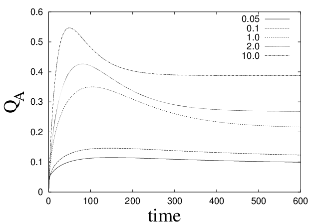
In the table II we give the relative height of the peak () for different
and , at high loading
(), where is the height of
the peak.
| case | ||||
|---|---|---|---|---|
| MF | Sim | |||
| a) | 0.01 | 2.0 | 1.5905 | 2.9521 |
| b) | 0.1 | 2.0 | 2.1590 | 2.693 |
| c) | 1.0 | 2.0 | 2.9911 | 2.9984 |
| d) | 0.01 | 0.05 | 1.4365 | 1.2761 |
| e) | 0.01 | 0.1 | 1.5070 | 1.4546 |
| f) | 0.01 | 1.0 | 1.6458 | 2.654 |
| g) | 0.01 | 2.0 | 1.5904 | 2.9384 |
| h) | 0.01 | 10.0 | 1.4095 | 3.141 |
| i) | 2.0 | 2.0 | 3.329 | 3.305 |
MF overestimates the height of this peak comparing with simulation results, but both DMC and MF results converge in the same way to steady-state. In figure 13 we show that MF results corresponds to DMC results for transients for slow reaction systems.

When difussion is slow and reaction is fast, MF predicts very well the DMC results. We have also in this case an overshoot for in the transient regime. When we have slow diffusion and very slow reaction, the height of the peak increases with both and (see table II for d, e, f). Also in this case the MF corresponds to the DMC results.
As MF ignores the spatial correlations between NN sites and MF gives qualitatively good results comparing with DMC results, we conclude that MF is a good enough approximation for the case when all the sites are reactive. This is confirmed also by the comparison between MF and Pair Approximation. The Pair Approximation gives the same results as MF.
III.3.2 Only some of the sites reactive
We want to see how the distribution of the reactive sites influence the relaxation of and loadings. We compare the MF and the DMC results for fast reaction and for slow reaction systems, for different distributions of the reactive sites. We distinguish homogeneous distribution of the reactive sites, marginal sites reactive, and middle sites reactive).
We have previously seen that for fast reaction systems and all sites reactive, the relaxation of and is the same as the relaxation of the total loading . From S.V.Nedea et al. 2002 we know that the results for the total loading, both for transients and for steady-state, can be derived analytically from exact equations and these results corresponds to the DMC results. When only the marginal sites are reactive and reaction very fast, DMC and MF results are similar with DMC and MF results for the cases when all sites are reactive and when it is a homogeneous distribution of the reactive sites in the pipe. When the reactive sites are situated in the middle of the pipe, the loadings ,and relax slower to equilibrium than in the case all the sites are reactive, because it takes more time for the particles to reach the reactive sites.
For slow reaction systems and all sites reactive, the relaxation of and is slower than the relaxation of the total loading . For this case we can not derive from exact equations. The loading is converging to equilibrium simultaneously with loading. We compare thus DMC and MF results for different distributions of the reactive sites, for different reaction rates. We will analyze two cases, the first for slow reaction () and the second for very slow reaction ().
In the first case (), the loading for homogenous distribution and middle site reactive reaches equilibrium faster than in the case of marginal sites reactive. This is happening because for marginal sites reactive, the ’s are formed near the open ends and, consequently, they can easily desorb and the equilibrium is reached later. When the marginal sites are reactive, the residence time of the ’s is small and the probability to find a on a marginal site is high. The loading with ’s is increasing more slowly to the steady-state value because of the ’s that are in the middle of the pipe. The same behavior has the loading converging to equilibrium simultaneously with loading. When the reactive sites are distributed in the middle of the pipe, because of blocking, the ’s can not reach easily the open ends, the probability to find a on a marginal site is small, and the residence time of the ’s in the system is large. The loading with ’s is increasing fast to the steady-state value. From figure 14, we see that and for homogeneous and middle sites reactive have the same relaxation.


In the case of very slow reaction (), when the marginal sites are reactive, the loading increases faster than in the case of homogeneous and middle sites reactive, till a certain time because particles can reach faster the reactive sites. While more ’s are formed, the loading is converging slower because the ’s can desorb relatively fast from the marginal sites, the residence time of the formed ’s is smaller than in the case when the reactive sites are in the middle of the pipe or homogeneously distributed (see figure 14). converges faster in case the middle sites are reactive than in the case of homogeneous distribution of the reactive sites.
We compare the time dependence of the loading and of the loading using DMC and MF for slow reaction systems and different rates of conversion when diffusion is fast (see figure 15).


We see that differences appear in the transient region as well as in the steady-state for all the distributions of the reactive sites but very prominent for marginal and middle sites reactive. In this case, for homogeneous distribution of the reactive sites the differences between MF and DMC are small (see figure 16).


For the other cases (fast reaction-slow diffusion, fast reaction-fast diffusion, slow reaction-slow diffusion), MF gives good results compared to DMC for all the distributions of the reactive sites. In figure 17 we compare the MF results for the transients for the case when five marginal sites are reactive.


We finally look at the site occupancy of the pipe. The MF profiles for marginal sites reactive show in the transient regime accumulation of the ’s in the middle of the pipe for a slow reaction system and fast diffusion. Because reaction is slow, the ’s can pass without reacting to the nonreactive sites. As the loading is increasing, the residence time of the particles increases, and the probability to find an in the middle of the pipe is decreasing because of blocking (see figure 18).

Dynamic Monte Carlo simulations show the same behavior. In figure 19 we see as well accumulation of particles in the middle of the pipe in the transient regime. As a consequence, until the equilibrium is reached the middle sites have different contribution to the occupancy in the pipe depending on their position. In the steady-state all the middle sites have the same contribution to the occupancy profiles S.V.Nedea et al. 2002.

IV Summary
We have used DMC and analytical techniques to study the properties of Single-File Systems in the transient regime.
We have derived exact equations to solve the relaxation time of the whole system (). We found that there are two regimes describing the dependence on diffusion of the relaxation time . The first regime is for slow diffusion, when decreases fast with increasing diffusion, and the second for fast diffusion, when slowly decreases with diffusion to a limiting value. We have analytically derived this limiting value of for infinitely-fast diffusion.
We have also studied the transients in the case with conversion. MF results show that there are two different behaviors determined by conversion. For fast reaction systems, the relaxation time of the loading with ’s () and ’s () is equal to the relaxation time of the total loading (). When has reached equilibrium, and have also reached equilibrium. For slow reaction systems, the total loading relaxes faster to equilibrium than the loading with ’s () and ’s (). The regime between reaching equilibrium and and reaching equilibrium we call the reaction limited regime. In the reaction limited regime, MF shows that not only reaction, but also desorption has a strong influence influence on the transients. We find that the relaxation of () as a function of desorption varies with reaction for low desorption rates and converges to a limiting value for very high rates of desorption.
DMC results shows several regimes for the transients, in the case all the sites are reactive. In the case diffusion is slow, the relaxation time is determined by diffusion. When diffusion is fast and the reaction slow, then the relaxation time is determined by reaction and when both are fast, relaxation time is determined by adsorption/desorption. For all these cases the simulations results for the transients match the MF results, except when we have low reaction rates and fast diffusion for both low and high loading. In this case MF overestimates the amount of ’s in the pipe both for transients and for steady-state. DMC and MF results indicate also an overshoot for both for high and low loadings in the transient regime, that appears as a consequence of the difference between diffusion and reaction rates constants.
When only some of sites are reactive, for fast reaction systems, MF gives good results compared to DMC for all the distributions of the reactive sites. When only the marginal sites are reactive and reaction very fast, DMC and MF results are similar with DMC and MF results for the cases when all sites are reactive and when it is a homogeneous distribution of the reactive sites in the pipe. When the reactive sites are situated in the middle of the pipe, the loadings , and relax slower to equilibrium than in the case all the sites are reactive, because it takes more time for the particles to reach the reactive sites.
For slow reactive systems, differences between DMC and MF results appear for transients for different distributions of the reactive sites when diffusion is fast, but are very prominent for marginal and middle sites reactive. For homogeneous distribution of the reactive sites the differences between MF and DMC are small. For slow reaction, we find that the loading for homogenous distribution and middle site reactive reaches equilibrium faster than in the case of marginal sites reactive. For very slow reaction, increases faster at the beginning than in the case of homogeneous and middle sites reactive and becomes slower as the ’s are formed. converges also faster in the case the middle sites are reactive than in the case of homogeneous distribution of the reactive sites.
V Acknowledgments
The authors thank Prof.dr. R.A. van Santen for many stimulating discussions.
VI Appendix
VI.1 Derivation of the equations for two-sites probabilities
In order to solve the rate equations of the system we use Cluster Approximation. For simplicity we consider an approximation that considers only the correlations between pairs of NN sites - Pair Approximation. To the already derived rate equations for one-site probabilities we add the two-site probability equations. We write write these equations in terms of three sites probabilities and we use then the decoupling scheme
| (47) |
We give here the equations for the two-site probabilities for and * occupancy of these sites. The equations for the left marginal sites are
| (48) |
where , etc.
Almost similar are the equations for the right marginal sites
| (49) |
And, finally, the equations for the non-marginal sites
| (50) |
We have the possibility to determine the one-site probabilities by calculating the sum of the two-sites probabilities
References
- Baxter (1982) R. J. Baxter, Exactly solved models in statistical mechanics (Academic Press, New York, 1982).
- Derrida and Evans (1997) B. Derrida and M. Evans, Cambridge University Press, U.K. (1997).
- Alcaraz (1994) F. C. Alcaraz, Int. J. Mod. Phys B 8, 3349 (1994).
- Derrida et al. (1992) B. Derrida, E. Domany, and D. Mukamel, J. Stat. Phys. 69, 667 (1992).
- Schutz and Domany (1993) G. Schutz and E. Domany, J. Stat. Phys. 72, 277 (1993).
- Derrida et al. (1993) B. Derrida, M. R. Evans, V. Hakim, and V. Pasquier, J. Phys. 26, 1493 (1993).
- J.G.Tsikoyannis and Wei (1991) J.G.Tsikoyannis and J. Wei, Chem. Eng. Sci. 46, 233 (1991).
- Rdenbeck et al. (1997) C. Rdenbeck, J. Krger, and K.Hahn, Physical Review E 55, 5697 (1997).
- Okino et al. (1999) M. S. Okino, R. Q. Snurr, H. H. Kung, J. E. Ochs, and M. L. Mavrovouniotis, J. Chem. Phys. 111, 2210 (1999).
- Coppens et al. (1998) M.-O. Coppens, A. Bell, and Chakraborty, Chem. Engng. Sci. 53, 2053 (1998).
- Coppens et al. (1999) M.-O. Coppens, A. Bell, and Chakraborty, Chem. Engng. Sci. 54, 3455 (1999).
- Privman (1997) V. Privman, Nonequilibrium statistical mechanics in one dimension (Cambridge University Press, U. K., 1997).
- Marro and Dickman (1998) J. Marro and R. Dickman, Nonequilibrium phase transitions in lattice models (Cambridge University Press, Cambridge, 1998).
- Dickman and Jensen (1991) R. Dickman and I. Jensen, Phys. Rev. Lett. 67, 2391 (1991).
- Grinstein et al. (1989) G. Grinstein, Z. W. Lai, and D. A. Browne, Phys. Rev. A 40, 4820 (1989).
- Dickman and Burschka (1988) R. Dickman and M. Burschka, Phys. Lett. A 127, 132 (1988).
- S.V.Nedea et al. (2002) S.V.Nedea, A.P.J.Jansen, J.J.Lukkien, and P.A.J.Hilbers, Phys.Rev.E (2002).
- Derrida and Evans (1999) B. Derrida and M. R. Evans, J. Phys. A 32, 4833 (1999).
- Ben-Naim and Krapivsky (1994) Ben-Naim and P. L. Krapivsky, J. Phys. A 27, 481 (1994).
- Derrida et al. (1996) B. Derrida, V. Hakim, and R. Zeitak, Phys. Rev. Lett. 77, 2871 (1996).
- J.Mai et al. (1994a) J.Mai, V. Kuzovkov, and W. von Niessen, J.Chem.Phys. 100(11), 8522 (1994a).
- von Smoluchowski (1917) M. von Smoluchowski, Z. Phys. Chem. 92, 129 (1917).
- Kampen (1981) V. Kampen, Stochastic Processes in Physics and Chemistry (Elsevier Science Publishers B.V., 1981).
- Mamada and Takano (1968) H. Mamada and F. Takano, J. Phys. Soc. Japan 25 25, 675 (1968).
- Lukkien et al. (1998) J. Lukkien, J. Segers, P.A.J.Hilbers, R.J.Gelten, and A.P.J.Jansen, Phys.Rev.E 58, 2598 (1998).
- R.J.Gelten et al. (1998a) R.J.Gelten, A.P.J.Jansen, R. van Santen, J.J.Lukkien, and P. Hilbers, J.Chem.Phys. 108(14), 5921 (1998a).
- R.J.Gelten et al. (1999) R.J.Gelten, R. van Santen, and A.P.J.Jansen, Dynamic Monte Carlo simulations of oscillatory heterogeneous catalytic reactions in P.B. Balbuena and J.M.Seminario (Elsevier, Amsterdam, 1999).
- R.J.Gelten et al. (1998b) R.J.Gelten, R. van Santen, and A.P.J.Jansen, Israel J.Chem. 38, 415 (1998b).
- A.P.J.Jansen (1995) A.P.J.Jansen, Comput. Phys. Comm. 86, 1 (1995).
- Segers (1999) J. Segers, Algorithms for the Simulation of Surface Processes (Ph.D. thesis, Eindhoven University of Technology, 1999).
- Binder (1986) K. Binder, Monte Carlo methods in Statistical Physics (Springer, Berlin, 1986).
- Gillespie (1976) D. Gillespie, J.Comput.Phys. 22, 403 (1976).
- Gillespie (1977) D. Gillespie, J.Phys.Chem. 81, 2340 (1977).
- J.Mai et al. (1994b) J.Mai, V. Kuzovkov, and W. von Niessen, J.Chem.Phys. 100(8), 6073 (1994b).
- Guttmann (1989) A. J. Guttmann, Asymptotic analysis of power-series expansions in Phase transitions and critical phenomena (Academic Press, 1989).
- Amit (1984) D. J. Amit, Field theory, the renormalization group, and critical phenomen (World Scientific, Singapore, 1984).
- Liggett (1985) T. M. Liggett, Interacting particle systems (Springer, Berlin, 1985).
- Spohn (1991) H. Spohn, Interacting particle systems (Springer, Berlin, 1991).
- McCoy and Wu (1973) B. M. McCoy and T. T. Wu, The two-dimensional Ising model (Harvard University Press, Cambridge, 1973).
- Polyakov (1970) A. M. Polyakov, Sov. Phys. JETP Lett. 12, 381 (1970).
- Cardy (1987) J. L. Cardy, Phase transitions and critical phenomena (Academic Press, New York, 1987).
- Henkel (1999) M. Henkel, Conformal Invariance and Critical Phenomena (Springer Verlag, Berlin, 1999).
- Schmittmann and Zia (1995) B. Schmittmann and R. K. P. Zia, Statistical mechanics of driven diffusive systems in Phase transitions and critical phenomen (Academic Press, New York, 1995).
- Alcaraz et al. (1994) F. C. Alcaraz, M. H. M. Droz, and V. Rittenberg, Ann. Phys. (N.Y. 230, 250 (1994).
- Evans et al. (1999) M. R. Evans, N. Rajewsky, and E. R. Speer, J. Stat. Phys 95, 45 (1999).
- Gwa and Spohn (1992) L. H. Gwa and H. Spohn, Phys. Rev. A 46, 844 (1992).
- Doering et al. (1991) C. R. Doering, M. A. Burschka, and W. Horsthemke, J. Stat. Phys. 65, 953 (1991).
*