Collisional deexcitation of exotic hydrogen atoms in highly excited states. I. Cross-sections

T.S. Jensen V.E. Markushin Affiliation: Paul Scherrer Institute, CH-5232 Villigen PSI, Switzerland Affiliation: Institut für Theoretische Physik der Universität Zürich, Winterthurerstrasse 190, CH-8057 Zürich, Switzerland

Received: date / Revised version: date

Abstract

The deexcitation of exotic hydrogen atoms in highly excited states in collisions with hydrogen molecules has been studied using the classical-trajectory Monte Carlo method. The Coulomb transitions with large change of principal quantum number $n$ have been found to be the dominant collisional deexcitation mechanism at high $n$ . The molecular structure of the hydrogen target is shown to be essential for the dominance of transitions with large $\Delta n$ . The external Auger effect has been studied in the eikonal approximation. The resulting partial wave cross-sections are consistent with unitarity and provide a more reliable input for cascade calculations than the previously used Born approximation.

pacs

34.50.-sScattering of atoms and molecules and 36.10.-kExotic atoms and molecules (containing mesons, muons, and other unusual particles)

1 Introduction

Exotic hydrogen atoms $x^{-}p$ ( $x^{-}=\mu^{-},\pi^{-},K^{-},\bar{p}$ ) are formed in highly excited states with the principal quantum number $n\sim\sqrt{\mbox{$\mu_{xp}$}/m_{e}}$ where $\mu_{xp}$ is the reduced mass of the exotic atom leon62; cohen99. For a long time the initial stage of the atomic cascade remained poorly understood despite a substantial progress in theoretical and experimental studies (see borie80; markushin94; markushin99 and references therein). In particular, the dominant collisional deexcitation mechanism was unclear for 40 years since the so-called chemical deexcitation was introduced in leon62 as a phenomenological solution to the problem of the cascade time at high $n$ (the external Auger effect alone would give much longer cascade times). A shortage of experimental data related to the initial stage of the atomic cascade hindered theoretical studies of this problem. The experimental situation, however, changed recently as more data on the atomic cascades in exotic hydrogen atoms at low density became available. The cascade time of antiprotonic hydrogen measured by the OBELIX collaboration obelix00 in the density range $3-150\;$ mbar was found to be significantly shorter than the prediction of the conventional cascade model reifenrother89. The new experimental results on the atomic cascade in muonic hydrogen from the PSI experiment kottmann99 provided detailed information not only on the cascade time, but also on the energy distribution at the end of the cascade, which at low density is actually preserved from the initial stage after the fast radiative deexcitation takes over the collisional processes.

The goal of this paper is to investigate the collisional deexcitation mechanisms for highly excited exotic atoms. In particular, we are interested in the role of the Coulomb acceleration in highly excited states and in the competition between the acceleration and slowing down in quasi-elastic collisions. Both molecular and atomic hydrogen targets were used in our calculations in order to investigate the role of molecular effects.

The paper is organized as follows. The classical-trajectory Monte Carlo method is described in Section 2. The results of calculations of Coulomb, Stark, and transport cross-sections for the $\mu^{-}p$ and $\bar{p}p$ atoms are presented in Section 3. The Auger deexcitation is discussed in Section 4. The conclusions are summarized in Section 5.

Unless otherwise stated, atomic units ( $\hbar=e=m_{e}=1$ ) are used throughout this paper. The unit of cross-section is $a_{0}^{2}=2.8\cdot 10^{-17}\;{\rm cm}^{2}$ , where $a_{0}=\frac{\hbar^{2}}{m_{e}e^{2}}$ is the electron Bohr radius.

2 Classical-trajectory Monte Carlo calculation

2.1 Effective potential

In the beginning of the atomic cascade, where many $nlm$ -states are involved in the collisions, classical mechanics is expected to be a good approximation. To study the scattering of exotic hydrogen atoms from hydrogen atoms or molecules we use a classical-trajectory Monte Carlo model. The following degrees of freedom are included in the model: the constituents of the exotic atom ( $x^{-}=\mu^{-},\pi^{-},K^{-},\bar{p}$ and the proton) and the hydrogen atoms are treated as classical particles. The electrons are assumed to have fixed charge distributions corresponding to the $1s$ atomic state around the protons in the hydrogen atoms.

We describe the exotic atom as a classical two-body system with the potential

\displaystyle V_{x^{-}p}(\mathbf{r})

\displaystyle=

\displaystyle-\frac{1}{r}.

(1)

The exotic atom interacts with two hydrogen atoms whose electron distributions are assumed to be frozen in the ground atomic state (see Figure 1 for notation):

	$\displaystyle V_{x^{-}p-H}(\mathbf{r},\mathbf{R})$	$\displaystyle=$	$\displaystyle\left(\frac{1}{R_{p}}+1\right)e^{-2R_{p}}$		(2)
		$\displaystyle-$	$\displaystyle\left(\frac{1}{R_{x}}+1\right)e^{-2R_{x}}$		(2)

The interaction between the hydrogen atoms is described by the Morse potential

\displaystyle V_{\mathrm{HH}}(\mathbf{R}_{\mathrm{HH}})

\displaystyle=

\displaystyle D_{e}(e^{-\alpha(R_{\mathrm{HH}}-R_{0})}-1)^{2}

(3)

where $D_{e}=4.75~\mathrm{eV}$ , $\alpha=1.03$ , and $R_{0}=1.4$ bransden83. The effective potential for the $\mbox{$x^{-}p$}+\mbox{${\mathrm{H}}$}+\mbox{${\mathrm{H}}$}$ system (see Figure 2) has the form

	$\displaystyle V$	$\displaystyle=$	$\displaystyle V_{x^{-}p}(\mathbf{r})+V_{x^{-}p-H}(\mathbf{r},\mathbf{R}_{1})+V_{x^{-}p-H}(\mathbf{r},\mathbf{R}_{2})$		(4)
		$\displaystyle+$	$\displaystyle V_{\mathrm{HH}}(\mathbf{R}_{\mathrm{HH}}).$		(4)

Refer to caption — Figure 1: Coordinates for the three-body subsystem. $C$ is the center of mass of the $x^{-}p$ .

2.2 Method of calculation

The classical equations of motion corresponding to the effective potential (4) were solved using a fourth-order Runge-Kutta method. The initial conditions were defined as follows. Given the initial principal quantum number $n_{i}$ and the orbital angular momentum $l_{i}$ of the $x^{-}p$ atom, the initial classical state was generated as a classical Kepler orbit with the total CMS energy $E_{xp}$ and the classical angular momentum $l_{c}$ :

	$\displaystyle E_{xp}$	$\displaystyle=$	$\displaystyle-\frac{\mbox{$\mu_{xp}$}}{2n_{i}^{2}},$		(5)
	$\displaystyle l_{c}$	$\displaystyle=$	$\displaystyle l_{i}+\frac{1}{2}.$		(6)

The orbit was oriented randomly in space, and the orbital $x^{-}p$ motion was set at a random time within the period. The hydrogen atoms in the target molecule were set at the equilibrium distance $R_{0}$ , and the molecule was randomly oriented in space. The impact parameter $\rho$ of the $x^{-}p$ atom was selected with a uniform distribution in the interval $(0,\rho_{\mathrm{max}})$ , as discussed below. The accuracy of the numerical calculations was controlled by checking the conservation of total energy and angular momentum. Instead of requiring convergence for every individual trajectory, we used the global criteria that the cross-sections for the various processes (see below) were stable within the statistical errors against further increase in the numerical accuracy for each collision.

The final atomic state was determined when the distance between $x^{-}p$ and the hydrogen atoms after the collision was larger than $10a_{0}$ . The final atomic state with the energy $E_{xp}$ and the angular momentum $l_{c}$ was identified as corresponding to the final $n_{f}l_{f}$ state according to the rules similar to (5,6):

	$\displaystyle n_{f}-\frac{1}{2}<$	$\displaystyle n_{c}=\sqrt{2\|E_{xp}\|/\mbox{$\mu_{xp}$}}$	$\displaystyle\leq n_{f}+\frac{1}{2}$		(7)
	$\displaystyle l_{f}<$	$\displaystyle l_{c}{n_{f}}/{n_{c}}$	$\displaystyle\leq l_{f}+1.$		(8)

In addition to the quantum numbers $n_{f}$ and $l_{f}$ , the CMS scattering angle $\theta$ and the excitation energy of the target $\Delta E_{\mathrm{target}}$ were also obtained. For the purpose of cascade calculations, we are mainly interested in the reaction channels that include the $x^{-}p$ atomic states:

\displaystyle(\mbox{$x^{-}p$})_{n_{i}l_{i}}+\mbox{${\mathrm{H}}$}_{2}

\displaystyle\to

\displaystyle\left\{\begin{array}[]{l}(\mbox{$x^{-}p$})_{n_{f}l_{f}}+\mbox{${\mathrm{H}}$}_{2}\\ (\mbox{$x^{-}p$})_{n_{f}l_{f}}+\mbox{${\mathrm{H}}$}_{2}^{*}\\ (\mbox{$x^{-}p$})_{n_{f}l_{f}}+\mbox{${\mathrm{H}}$}+\mbox{${\mathrm{H}}$}\end{array}\right.

Other possible channels are the breakup reactions

\displaystyle(\mbox{$x^{-}p$})_{n_{i}l_{i}}+\mbox{${\mathrm{H}}$}_{2}

\displaystyle\to

\displaystyle\left\{\begin{array}[]{l}x^{-}+p+\mbox{${\mathrm{H}}$}_{2}^{*}\\ x^{-}+p+\mbox{${\mathrm{H}}$}+\mbox{${\mathrm{H}}$}\end{array}\right.

and the formation of $(x^{-}\mbox{${\mathrm{H}}$})_{n_{f}l_{f}}$ ions

(\mbox{$x^{-}p$})_{n_{i}l_{i}}+\mbox{${\mathrm{H}}$}_{2}\to(x^{-}\mbox{${\mathrm{H}}$})_{n_{f}l_{f}}+p+\mbox{${\mathrm{H}}$}.

(16)

An example of a collision that results in Coulomb deexcitation of the $\mu^{-}p$ and dissociation of the hydrogen molecule is shown in Figure 3.

For a given initial $n$ of the $x^{-}p$ and laboratory kinetic energy, $T_{i}$ , a set of the impact parameters $\rho_{i},\;i=1,...,K$ with a uniform distribution in the interval $(0,\rho_{\mathrm{max}})$ was generated. The value $\rho_{\mathrm{max}}=5+2n_{i}^{2}/\mbox{$\mu_{xp}$}$ was found to be suitable for all cases concerned. The cross-sections were obtained from the computed set of trajectories using the following procedure. Let $P_{i}^{\alpha}$ be the probability that the reaction channel $\alpha$ corresponds to the final state in collision $i$ :

\displaystyle P_{i}^{\alpha}

\displaystyle=

\displaystyle\left\{\begin{array}[]{rcl}1&,&\mbox{\rm if $\alpha$ occurred}\\ 0&,&\mbox{\rm otherwise}\end{array}\right.

The cross-section for the reaction channel $\alpha$ is given by

\displaystyle\sigma_{\alpha}

\displaystyle=

\displaystyle 2\pi\rho_{\mathrm{max}}\frac{1}{K}\sum_{i=1}^{K}\rho_{i}P_{i}^{\alpha}

(20)

The differential cross-sections are determined in a similar way by binning the corresponding intervals of variables like $z=\cos\theta$ , where $\theta$ is the CMS scattering angle, and the target excitation energy $\Delta E_{\mathrm{target}}$ . For instance, the differential cross-section $\mbox{\rm d}\sigma(z)/\mbox{\rm d}z$ is calculated using the relation

\frac{\mbox{\rm d}\sigma(z)}{\mbox{\rm d}z}\approx\frac{\sigma(z-\Delta z<\cos\theta<z+\Delta z)}{2\Delta z}

(21)

2.3 Special final states

The formation of $x^{-}\mathrm{H}$ ions in reaction (16) is an artifact of our model due to the treatment of the electrons as fixed charge distributions. The cross-sections for these processes turn out to be small, and usually the final $n_{f}$ is small, so that the electron screening is not very important. For the purpose of cascade calculations, one can count the $x^{-}\mathrm{H}$ formation as the $x^{-}p$ events with the corresponding values of $n_{f}$ , $l_{f}$ , $\cos\theta$ , and $\Delta E_{\mathrm{target}}$ . Another channel involving $x^{-}\mathrm{H}$ ions is related to the formation of metastable molecular states like

p(x^{-}\mathrm{H})_{n_{f}l_{f}}

(22)

where a deeply bound $x^{-}\mbox{${\mathrm{H}}$}$ ion forms a loosely bound state with the proton. These molecular states can be rather stable and often do not dissociate within a reasonable amount of computer time. In our calculations we consider the metastable molecular states as final states. We used the following criteria for the metastability: first, the collision time must exceed

t_{\mathrm{mol}}=50/v_{\mathrm{init}}

(23)

where $v_{\mathrm{init}}$ is the initial velocity of the $x^{-}p$ in the laboratory system. With the choice of the time interval (23), the colliding particles reach their asymptotically free final trajectories for most non-resonant collisions. Second, the $x^{-}$ must form a bound state with one of the hydrogen atoms and the binding energy must not vary by more than 1% within the time

\tau=20\frac{2\pi n_{i}^{3}}{\mbox{$\mu_{xp}$}}

(24)

which corresponds to 20 classical periods of the initial $x^{-}p$ atom. Once metastability is reached, the event is counted as an $x^{-}\mathrm{H}$ event.

3 Results

The classical-trajectory Monte Carlo method described in Section 2 has been used to obtain the collisional cross-sections needed in calculations of the cascades in $\mu^{-}p$ , $\pi^{-}p$ , $K^{-}p$ , and $\bar{p}p$ . The same method can also be used in a direct simulation of the atomic cascade without using pre-calculated cross-sections. For $\mu^{-}p$ and $\bar{p}p$ atoms experimental data at low density are available for direct comparison with the cascade calculations jensen02next. We will, therefore, present detailed results for these two cases. The initial stages also affect the cascades in $\pi^{-}p$ and $K^{-}p$ because they determine the kinetic energy distribution in the intermediate stage of the cascade where nuclear absorption becomes important.

The calculations have been done for $n_{i}=8-20$ for $\mu^{-}p$ , $n_{i}=13-35$ for $\bar{p}p$ and 9 values of the laboratory kinetic energy in the interval $0.05\;\mbox{\rm eV}\leq T\leq 20\;\mbox{\rm eV}$ . At $T=1\;\mbox{\rm eV}$ the cross-sections have been calculated down to $n_{i}=4$ for $\mu^{-}p$ and $n_{i}=8$ for $\bar{p}p$ . For each initial state $(n_{i},T)$ , 1000 classical trajectories have been calculated as described above. The orbital quantum number $l_{i}$ was distributed according to the statistical weight. For the purpose of illustration, a larger number of trajectories (up to 10000) have been calculated for some initial states in order to reduce statistical errors. Preliminary results have been shown in jensen02hyp.

We compare the results of the classical Monte Carlo (CMC) calculations with those of the semiclassical approximation. Bracci and Fiorentini bracci78 calculated the Coulomb cross-sections for muonic hydrogen scattering from atomic hydrogen in a semiclassical model. Though the approach bracci78 may be unsuitable for treating the low $n$ states, where more elaborate calculations give much smaller values for the cross-sections ponomarev99, it can be expected to give a fair description of the high $n$ region. In the case of Stark mixing we use the fixed field model jensen02epjd for comparison. In the case of molecular target, we obtained a semiclassical estimate of the Stark cross-sections by using the spherical symmetric electric field corresponding to the charge distribution of a $\mbox{${\mathrm{H}}$}_{2}$ molecule in the ground state.

3.1 Muonic hydrogen

3.1.1 Coulomb deexcitation

The $n$ dependences of the total cross-sections of the Coulomb deexcitation for collisions with molecular and atomic hydrogen

	$\displaystyle(\mbox{$x^{-}p$})_{n_{i}l_{i}}+\mbox{${\mathrm{H}}$}_{2}$	$\displaystyle\to$	$\displaystyle\left\{\begin{array}[]{l}(\mbox{$x^{-}p$})_{n_{f}l_{f}}+\mbox{${\mathrm{H}}$}_{2}^{*}\\ (\mbox{$x^{-}p$})_{n_{f}l_{f}}+\mbox{${\mathrm{H}}$}+\mbox{${\mathrm{H}}$}\end{array}\right.,$
	$\displaystyle(\mbox{$x^{-}p$})_{n_{i}l_{i}}+\mbox{${\mathrm{H}}$}$	$\displaystyle\to$	$\displaystyle(\mbox{$x^{-}p$})_{n_{f}l_{f}}+\mbox{${\mathrm{H}}$}$		(28)

with $n_{f}<n_{i}$ are shown in Figure 4. The cross-sections increase steadily with increasing $n$ as the $\mu^{-}p$ becomes larger and the energy spacing between the $n$ levels smaller. The cross-sections for the atomic target at the laboratory kinetic energy $T=1\;$ eV are very close to the semiclassical results of Bracci and Fiorentini bracci78. The cross-section for the molecular target is larger by a factor of about $2-3$ .

An example of the energy dependence of the total Coulomb cross-sections ( $n_{f}<n_{i}$ ) for $n_{i}=13$ is shown in Figure 5. The cross-sections calculated with molecular target are approximately twice as large as the atomic ones in the whole energy range considered. The CMC result for the atomic target is in fair agreement with the semiclassical result bracci78 for energies above 1 eV. The energy dependence of the CMC cross-sections is approximately given by $1/\sqrt{T}$ corresponding to constant rates. This is in contrast to the $1/T$ behavior found for low energies in bracci78.

The distribution over final states $n_{f}$ is completely different for the molecular and the atomic targets as illustrated in Figure 6 showing the $l$ -average cross-sections $\sigma_{13\to n_{f}}$ for $\mu^{-}p$ at 1 eV. The calculations for atomic target predict that $\Delta n=1$ transitions dominate the Coulomb deexcitation in agreement with the semiclassical result bracci78. For the molecular target, the transitions with $\Delta n>1$ are strongly enhanced as compared to the atomic case. The shape of the $n_{f}$ distribution depends on the initial state $n_{i}$ : with decreasing $n_{i}$ it becomes narrower and its maximum shifts towards smaller values of $\Delta n$ . For $n_{i}=13$ , the transitions $\Delta n=2-3$ dominate. Figure 7 shows the $n_{f}$ dependence for initial state $n_{i}=9$ : the transitions with $\Delta n=1$ are most likely, but the $\Delta n>1$ transitions still make up a substantial fraction of 38% of the Coulomb cross-section as compared to 19% for atomic target.

3.1.2 Stark mixing and elastic scattering

The Stark collisions change the orbital angular momentum while preserving the principal quantum number:

	$\displaystyle(\mbox{$x^{-}p$})_{n_{i}l_{i}}+\mbox{${\mathrm{H}}$}_{2}$	$\displaystyle\to$	$\displaystyle\ (\mbox{$x^{-}p$})_{n_{i}l_{f}}+\mbox{${\mathrm{H}}$}_{2}^{*}\;(\mbox{${\mathrm{H}}$}+\mbox{${\mathrm{H}}$}),$		(29)
	$\displaystyle(\mbox{$x^{-}p$})_{n_{i}l_{i}}+\mbox{${\mathrm{H}}$}$	$\displaystyle\to$	$\displaystyle(\mbox{$x^{-}p$})_{n_{i}l_{f}}+\mbox{${\mathrm{H}}$}.$		(30)

The CMC results for the $n$ dependence of the $l$ -average Stark mixing cross-section are shown in Figure 8. The Stark cross-sections calculated with molecular target are less than twice the atomic ones. This is due to two reasons. First, there is a considerable molecular screening effect because the electric fields from the two hydrogen atoms partly cancel each other. Second, the Coulomb cross-section makes up a larger fraction of the total cross-section in the molecular case. The classical Monte Carlo results for the atomic target are in a good agreement with the semiclassical fixed field model. At low $n$ , where the inelasticity due to the Coulomb deexcitation is small and can be neglected in the calculation of the Stark cross-sections, there is a good agreement between the classical Monte Carlo results for the molecular target and the corresponding semiclassical model.

Figure 9 shows the energy dependence of the Stark cross-sections for $n=9$ . The classical-trajectory model and fixed field model are in agreement with each other for kinetic energies above 10 eV (molecular target) and 2 eV (atomic target). At lower energies where the Coulomb transitions make up a substantial part of the cross-sections, the fixed field model overestimates the Stark cross-sections.

The Stark mixing and elastic scattering processes, (29) and (30), lead to a deceleration of the exotic atom. Their importance in the kinetics of atomic cascade can be estimated with the corresponding transport cross-section

\sigma_{n}^{\mathrm{tr}}=\int(1-\cos\theta)\frac{\mbox{\rm d}\sigma_{n\to n}}{\mbox{\rm d}\Omega}\mbox{\rm d}\Omega

(31)

where $\mathrm{d}\sigma_{n\to n}/\mathrm{d}\Omega$ is the differential cross-section for the processes (29) or (30) averaged over $l$ . This estimate based on the transport cross-section neglects the Coulomb deexcitation process which can lead to both deceleration and acceleration, and, in the case of molecular target, the additional deceleration due to excitation of the $\mbox{${\mathrm{H}}$}_{2}$ molecule. The $n$ dependence of the transport cross-sections at 1 eV for muonic hydrogen scattering from hydrogen atoms and molecules is shown in Figure 10. There is a fair agreement between the CMC and the fixed field model for atomic target below $n\sim 8$ . For higher $n$ , the inelastic effects due to the Coulomb deexcitation process become important, and the fixed field model overestimates the transport cross-section. For molecular target, the discrepancy between the two models is larger because the Coulomb cross-section makes up a larger fraction of the total cross-section as compared to the CMC model with atomic target (for $n=10$ and $T=1$ eV the fractions are $\sim 0.24$ for molecular target and $\sim 0.11$ for atomic target).

Figure 11 shows the $l$ -averaged differential cross-section (using 20 equally spaced bins in $z$ ) summed over all the final channels for $n_{i}=13$ in the classical Monte Carlo model with atomic target. The cross-section is in good agreement with that of the semiclassical fixed field model. The pattern of maxima and minima in the semiclassical differential cross-sections is a characteristic feature of quantum mechanical scattering, which, of course, cannot be reproduced in a classical model.

The kinetic energy of the $x^{-}p$ in the final state is important for detailed cascade calculations. Let $T_{x^{-}p}$ , $T_{\mathrm{H}}$ and $T_{\mathrm{H}_{2}}$ be the CMS kinetic energies of the $x^{-}p$ , the H (for atomic target), and the $\mathrm{H}_{2}$ (for molecular target). The total kinetic energy is shared among the two ( $x^{-}p$ and H) or three atoms ( $x^{-}p$ and two hydrogen atoms):

T_{\mathrm{tot}}=\left\{\begin{array}[]{ll}T_{x^{-}p}+T_{\mathrm{H}},&{\rm atomic\;target}\\ T_{x^{-}p}+T_{\mathrm{H}_{2}}+\Delta E_{\mathrm{target}},&{\rm molecular\;target}\end{array}\right.

(32)

In the case of atomic target, the energy of the $x^{-}p$ in CMS is fixed:

\frac{T_{x^{-}p}}{T_{\mathrm{tot}}}=\frac{M_{\mathrm{H}}}{M_{xp}+M_{\mathrm{H}}}\quad(=0.47\;\mathrm{for}\;\mbox{$\mu^{-}p$})

(33)

where $M_{\mathrm{H}}$ and $M_{xp}$ are the masses of the hydrogen atom and the $x^{-}p$ atom, correspondingly. The case of molecular target corresponds to a three-body final state with the kinematical boundaries:

0\leq\frac{T_{x^{-}p}}{T_{\mathrm{tot}}}\leq\frac{T_{x^{-}p}^{\mathrm{max}}}{T_{\mathrm{tot}}}=\frac{2M_{\mathrm{H}}}{M_{xp}+2M_{\mathrm{H}}}.

(34)

The upper boundary (0.64 for muonic hydrogen) is reached when the hydrogen molecule remains in its ground state corresponding effectively to a two-body ( $(\mbox{$x^{-}p$})+(\mbox{${\mathrm{H}}$}_{2})$ ) final state. Figure 12 shows the distributions in $T_{x^{-}p}/T_{\mathrm{tot}}$ for Coulomb deexcitations calculated in the classical Monte Carlo model for muonic hydrogen with $n_{i}=9$ , 13 and $T=1$ eV. The approximation of effective two-body final states clearly fails, whereas the pure phase space distribution

f(T_{x^{-}p})=\frac{4T_{\mathrm{tot}}}{\pi T_{x^{-}p}^{\mathrm{max}}}\sqrt{1-\left(\frac{2T_{x^{-}p}}{T_{x^{-}p}^{\mathrm{max}}}-1\right)^{2}}

(35)

gives a fair description of the results.

3.2 Antiprotonic hydrogen

The atomic cascade in antiprotonic hydrogen starts around $n_{i}\sim 30$ ; thus classical mechanics is even a better approximation than in the muonic hydrogen case. The $n$ dependence of the Stark mixing, Coulomb deexcitation, transport, and the $\bar{p}\mbox{${\mathrm{H}}$}$ formation cross-sections is shown in Figure 13, and the energy dependence is demonstrated in Figure 14. As with muonic hydrogen, the fixed field model overestimates the Stark mixing and especially the transport cross-section because the inelasticity effects due to Coulomb deexcitation are not included in this framework.

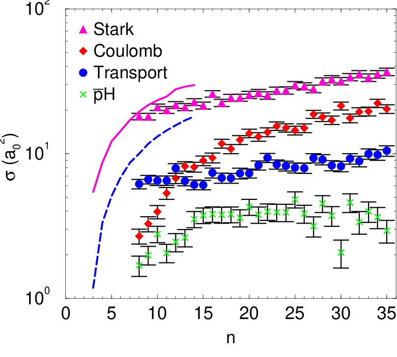
Figure 15 shows the distribution over the final states $n_{f}$ for the Coulomb deexcitation of the antiprotonic hydrogen at the laboratory energy $T=1$ eV. For high $n$ initial states, the most probable Coulomb transitions are the ones with a large change of the principal quantum number ( $\Delta n\gg 1$ ), with the molecular target being essential for this feature. A very important consequence of this result is that at the beginning of the atomic cascade a small number of Coulomb transitions is sufficient to bring the $\bar{p}p$ to the middle stage, where, depending on the target density, the radiative or Auger deexcitation takes over.

The dependence of the Coulomb cross-sections on the angular momentum $l_{i}$ of the initial state is weak, see Figure 16 for antiprotonic hydrogen with $n_{i}=25$ . The Stark cross-sections show a moderate dependence on $l_{i}$ : they are smaller for the circular states ( $l_{i}=n_{i}-1$ ) than for the low $l_{i}$ , by about 50%. The reason for this is that the elongated ellipses in the low $l$ states are more easily perturbed by the electric field of the target molecule. A similar effect is expected if a quantum mechanical description of the $\bar{p}p$ is used: the size of the $\bar{p}p$ as estimated by the expectation value of $r^{2}$ is given by

\langle r^{2}\rangle=\frac{n^{2}}{2\mu_{\mbox{$\bar{p}p$}}^{2}}\left(5n^{2}+1-3l(l+1)\right).

(36)

For high $n$ states, the expectation value of $r^{2}$ for the circular state is only 40% of that of the $ns$ states.

4 External Auger effect in the eikonal approximation

In our treatment of the Coulomb and Stark mixing collisions in Section 2, the electronic degrees of freedom were assumed to be frozen. These degrees of freedom, however, play an important role in the Auger deexcitation process

(x^{-}p)_{n_{i}l_{i}}+\mathrm{H}\to(x^{-}p)_{n_{f}l_{f}}+p+e^{-}.

(37)

The Auger transitions are often treated in the Born approximation leon62 that gives (conveniently) energy independent rates. However, this approximation violates unitarity for some important ranges of principal quantum numbers and kinetic energies. For kinetic energies in the range of few eV, the eikonal approximation bukhvostov82 provides a more suitable framework. In this section, we use the eikonal approach to calculate Stark mixing and Auger deexcitation simultaneously. As a result, the corresponding partial wave cross-sections are consistent with unitarity.

The cross-section for the process (37) was calculated in bukhvostov82 by assuming that the exotic atom moves along a straight line trajectory with constant velocity $v$ through the electric field of the hydrogen atom at rest. The cross-section is given by

\sigma^{\mathrm{Auger}}_{n_{i}l_{i}}=2\pi\int_{0}^{\infty}P(\rho)\rho\mbox{\rm d}\rho

(38)

where $P(\rho)$ is the reaction probability for the impact parameter $\rho$ :

P(\rho)=1-e^{-I(\rho)},\quad I(\rho)=\frac{1}{v}\int_{-\infty}^{\infty}\Gamma_{n_{i}l_{i}}(\sqrt{\rho^{2}+z^{2}})\mbox{\rm d}z.

(39)

The reaction rate, $\Gamma_{n_{i}l_{i}}(R)$ , at distance $R$ is the sum of the partial rates $\Gamma_{n_{i}l_{i}\to n_{f}l_{f}}(R)$ over all final states. According to bukhvostov82 the estimated rates are

\Gamma_{n_{i}l_{i}\to n_{f}l_{f}}(R)=\gamma\frac{1}{(R^{2}+b^{2})^{3}}+\gamma_{1}\frac{k_{e}^{2}}{1+k_{e}^{2}}\exp(-2R)

(40)

where $k_{e}$ is the electron momentum, $b=1.5$ , and the parameters $\gamma$ and $\gamma_{1}$ are given by

$\displaystyle\gamma$	$\displaystyle=$	$\displaystyle\frac{2^{10}\pi}{3}\mu_{xp}^{-2}\frac{\exp\left((-4/k_{e})\arctan k_{e}\right)}{(1+k_{e}^{2})^{6}(1-\exp(-2\pi/k_{e}))}$	(41)
	$\displaystyle\times$	$\displaystyle(C^{l_{f}0}_{l_{i}010})^{2}(R_{n_{i}l_{i}}^{n_{f}l_{f}})^{2},$	(41)
$\displaystyle\gamma_{1}$	$\displaystyle=$	$\displaystyle\frac{16}{3k_{e}}\mbox{$\mu_{xp}$}^{-2}(C^{l_{f}0}_{l_{i}010})^{2}(R_{n_{i}l_{i}}^{n_{f}l_{f}})^{2}$	(42)

where $C^{l_{f}0}_{l_{i}010}$ is a Clebsch-Gordan coefficient and $R_{n_{i}l_{i}}^{n_{f}l_{f}}$ is the radial matrix element bethe57. The transition rate is proportional to the square of the dipole matrix element, therefore only transitions with $\Delta l=|l_{f}-l_{i}|=1$ are possible.

The Auger deexcitation rate, as a function of $n$ , peaks at the $n$ -value where the energy released in a $\Delta n=1$ transition is just sufficient to ionize the hydrogen atom. The effect of these high-rate Auger transitions is that the inelastic cross-sections for some partial waves are not small in comparison with the unitarity limit. Therefore the corresponding inelasticity should be taken into account in the calculations of other collisional processes. One can expect that taking the Auger effect into account will reduce the other inelastic cross-sections. In order to examine this effect, we include the Auger deexcitation in the framework presented in jensen02epjd for calculating Stark mixing and elastic scattering. In the same way as the nuclear absorption processes in hadronic atoms were taken into account via imaginary energy shifts of the $ns$ -states, the Auger deexcitation process is included via the imaginary absorption potential, $-i\Gamma_{nl}(R)/2$ . The calculations can be done in the close-coupling model, the semiclassical model, and the fixed field model. In the case of the fixed field model, the time-dependent Schrödinger equation for the set of the linear independent solutions forming the $n^{2}\times n^{2}$ matrix $A$ is given by

i\dot{A}(t)=H(t)A(t)

(43)

where the interaction is given by

	$\displaystyle H(t)$	$\displaystyle=$	$\displaystyle Z\frac{1}{R^{2}(t)}(1+2R(t)+2R^{2}(t))e^{-2R(t)}$		(44)
		$\displaystyle+$	$\displaystyle\Delta E-i\frac{\Gamma(R)}{2}.$		(44)

Here $\Delta E$ is a diagonal matrix corresponding to the energy shifts due to the vacuum polarization and the strong interaction. The term $\Gamma(R)$ is a diagonal matrix with the matrix elements $\Gamma_{nl}(R)$ . The factor $Z$ originates from the dipole operator and has the following matrix elements ( $i=|nl\Lambda\rangle$ , $j=|n(l-1)\Lambda\rangle$ ):

Z_{ij}=-\frac{3n}{2\mu_{xp}}\sqrt{\frac{(l^{2}-\Lambda^{2})(n^{2}-l^{2})}{(2l+1)(2l-1)}}.

(45)

The solution of Equation (43) using the method described in jensen02epjd gives the scattering matrix $S^{\mathrm{FF}}$ . The cross-sections for the transitions $n_{i}l_{i}\to n_{i}l_{f}$ are given by

	$\displaystyle\sigma_{n_{i}l_{i}\to n_{i}l_{f}}$	$\displaystyle=$	$\displaystyle\frac{1}{2l_{i}+1}\frac{\pi}{k^{2}}\sum_{J}(2J+1)$
	$\displaystyle\times$	$\displaystyle\sum_{\Lambda}$	$\displaystyle\|\langle n_{i};JM\Lambda l_{f}\|S^{\mathrm{FF}}-1\|n_{i};JM\Lambda l_{i}\rangle\|^{2}$		(46)

and the ones of the Auger deexcitation by

	$\displaystyle\sigma_{n_{i}l_{i}}^{\mathrm{Auger}}$	$\displaystyle=$	$\displaystyle\frac{1}{2l_{i}+1}\frac{\pi}{k^{2}}\sum_{J}(2J+1)\Big((2l_{i}+1)$		(47)
		$\displaystyle-$	$\displaystyle\sum_{\Lambda l_{f}}\|\langle n_{i};JM\Lambda l_{f}\|S^{\mathrm{FF}}\|n_{i};JM\Lambda l_{i}\rangle\|^{2}\Big).$		(47)

We will refer to this framework as the eikonal multichannel model.

The $l$ -average Auger deexcitation cross-sections calculated with the method of bukhvostov82 (Equations (38) and (39)) agree closely with our results in the eikonal multichannel model. Figure 17 shows the $l$ -average $\Delta n=1$ Auger deexcitation rates in muonic hydrogen for $n=3,5,7$ . The rates have been calculated in the eikonal approximation and the Born approximation. The rates in the eikonal approximation are lower in the low energy range, but they approach the ones of the Born approximation for high energies. The $n$ dependence of the Auger deexcitation and Stark mixing rates for muonic hydrogen is presented in Figure 18. The two approaches are in a fair agreement with each other except for the states $n=6,7$ where the Auger rates have the highest values. For the state $n=7$ , the Stark mixing rates are reduced by almost 50% when the inelasticity due to the Auger effect is included. This resembles the situation with the eikonal and the Born approximations which disagree when the Auger deexcitation cross-sections are large, in which case the eikonal approximation gives smaller cross-sections than the Born approximation. The explanation of this effect is given in Figure 19 showing the average partial wave cross-sections for the collision $(\mu p)_{n=7}+\mbox{${\mathrm{H}}$}$ . The Auger deexcitation cross-sections are saturated in the low angular momentum region and, therefore, the Born approximation fails. Though the $l$ -average results agree for the two eikonal approaches, the $l$ dependence of the cross-sections in the eikonal multichannel model is weaker because of the effect of Stark mixing as demonstrated in Figure 20.

The eikonal approximation as described above does not give the differential cross-section and distribution over final $l_{f}$ for the Auger transitions. The partial wave cross-sections, Figure 19, show that the main contribution to the Auger cross-section comes from low partial waves, i.e. from the strong mixing region. This suggests that the distribution in $l_{f}$ is nearly statistical and that the differential cross-section is less forward-peaked than the elastic and Stark differential cross-sections jensen02epjd.

5 Conclusions

The collisional deexcitation mechanisms of the exotic hydrogen atoms in highly excited states have been investigated in detail using the classical-trajectory Monte Carlo method. The Coulomb transitions have been shown to be the dominant mechanism of collisional deexcitation of highly excited exotic atoms. Target molecular structure has large effects on the Coulomb deexcitation. In particular, the distribution over the final states favors large change of the principal quantum number $n$ contrary to the case of atomic target. This feature is very important for the cascade kinetics as it leads to a fast deexcitation and a significant acceleration at the initial stage of the atomic cascade jensen02next. The calculated cross-sections provide a more reliable theoretical input for further cascade studies by removing the long standing puzzle of the so-called chemical deexcitation leon62, which was used, on purely phenomenological grounds, in many cascade calculations without clarification of underlying dynamics.

The external Auger effect has been studied in an eikonal multichannel model which allows us to calculate Stark mixing, elastic scattering, and Auger deexcitation simultaneously. Partial wave cross-sections computed in this framework are consistent with unitarity. For ranges of principal quantum numbers and kinetic energies where the unitarity constraint is important, the Auger cross-sections computed in this model are significantly lower than those of the Born approximation leon62.

The first results of cascade calculations using the cross-sections of jensen02epjd and the present paper have been presented in markushin02hyp; jensen02pin. More detailed results of the cascade calculations will be discussed in a separate publication jensen02next.

Acknowledgment

We thank F. Kottmann, L. Simons, D. Taqqu, and R. Pohl for fruitful and stimulating discussions.

References

[1] M. Leon and H.A. Bethe, Phys. Rev. 127, 636 (1962).
[2] J.S. Cohen, Phys. Rev. A 59, 1160 (1999).
[3] E. Borie and M. Leon, Phys. Rev. A 21, 1460 (1980).
[4] V.E. Markushin, Phys. Rev. A 50, 1137 (1994).
[5] V.E. Markushin, Hyperf. Interact. 119, 11 (1999).
[6] A. Bianconi et al., Phys. Lett. B 487, 224 (2000).
[7] G. Reifenröther and E. Klempt, Nucl. Phys. A 503, 885 (1989).
[8] F. Kottmann et al., Hyperf. Interact. 119, 3 (1999).
[9] B.H. Bransden and C.J. Joachain, Physics of atoms and molecules (Longman Scientific & Technical, Essex, 1983).
[10] T.S. Jensen and V.E. Markushin, next paper.
[11] T.S. Jensen and V.E. Markushin, Proceedings of $\mu$ CF01, in press.
[12] L. Bracci and G. Fiorentini, Nuovo Cimento A 43, 9 (1978).
[13] L.I. Ponomarev and E.A. Solov’ev, Hyperf. Interact. 119, 55 (1999).
[14] T.S. Jensen and V.E. Markushin, Eur. Phys. J. D 19, 165 (2002).
[15] A.P. Bukhvostov and N.P. Popov, Sov. Phys. JETP 55, 12 (1982).
[16] H.A. Bethe and E.E. Salpeter, Quantum mechanics of one- and two-electron atoms (Academic Press, New York, 1957).
[17] V.E. Markushin and T.S. Jensen, Proceedings of $\mu$ CF01, in press.
[18] T.S. Jensen and V.E. Markushin, $\pi N$ Newsletter 16, 358 (2002).