A Local Ensemble Kalman Filter for Atmospheric Data Assimilation
Revised August 11, 2026
Abstract
In this paper, we introduce a new, local formulation of the ensemble Kalman Filter approach for atmospheric data assimilation. Our scheme is based on the hypothesis that, when the Earth’s surface is divided up into local regions of moderate size, vectors of the forecast uncertainties in such regions tend to lie in a subspace of much lower dimension than that of the full atmospheric state vector of such a region. Ensemble Kalman Filters, in general, assume that the analysis resulting from the data assimilation lies in the same subspace as the expected forecast error. Under our hypothesis the dimension of this subspace is low. This implies that operations only on relatively low dimensional matrices are required. Thus, the data analysis is done locally in a manner allowing massively parallel computation to be exploited. The local analyses are then used to construct global states for advancement to the next forecast time. The method, its potential advantages, properties, and implementation requirements are illustrated by numerical experiments on the Lorenz-96 model. It is found that accurate analysis can be achieved at a cost which is very modest compared to that of a full global ensemble Kalman Filter.
1 Introduction
The purpose of this paper is to develop and test a new atmospheric data assimilation scheme, which we call the Local Ensemble Kalman Filter method. Atmospheric data assimilation (analysis) is the process through which an estimate of the atmospheric state is obtained by using observed data and a dynamical model of the atmosphere (e.g., Daley 1991; Kalnay 2002). These estimates, called analyses, can then be used as initial conditions in operational numerical weather predictions. In addition, diagnostic studies of atmospheric dynamics and climate are also often based on analyses instead of raw observed data.
The analysis at a given time instant is an approximation to a maximum likelihood estimate of the atmospheric state in which a short-term forecast, usually referred to as the background or first guess field, is used as a prior estimate of the atmospheric state (Lorenc 1986). Then the observations are assimilated into the background field by a statistical interpolation. This interpolation is performed based on the assumptions (i) that the uncertainties in the background field and the observations are unbiased and normally distributed, (ii) that there are no cross correlations between background and observations errors, and (iii) that the covariance between different components of the background (formally the the background covariance matrix) and the covariances between uncertainties in the noisy observations (formally the observational error covariance matrix) are known. In reality, however, the background error covariance matrix cannot be directly computed. The implementation of a data assimilation system, therefore, requires the development of statistical models that can provide an estimate of the background error covariance matrix. The quality of a data assimilation system is primarily determined by the accuracy of this estimate.
In the case of linear dynamics the mathematically consistent technique to define an adaptive background covariance matrix is the Kalman Filter (Kalman 1960; Kalman and Bucy 1961) which utilizes the dynamical equations to evolve the most probable state and the error covariance matrix in time. In the case of linear systems with unbiased normally distributed errors the Kalman Filter provides estimates of the system state that are optimal in the mean square sense. The method has also been adapted to nonlinear systems, but, in this case, optimality no longer applies. Although the Kalman Filter approach has been successfully implemented for a wide range of applications and has been considered for atmospheric data assimilation for a long while (Jones 1965; Petersen 1973; Ghil et al. 1981, Dee et al., 1985), the computational cost involved does not allow for an operational implementation in the foreseeable future (see Daley 1991 for details).
The currently most popular approach to reduce the cost of the Kalman Filter is to use a relatively small (10-100 member) ensemble of background forecasts to estimate the background error covariances (e.g. Evensen 1994; Houtekamer and Mitchell 1998, 2001; Bishop et al. 2001; Hamill et al. 2001; Whitaker and Hamill 2002; Keppenne and Rienecker 2002). In ensemble-based data assimilation schemes the ensemble of background forecasts is generated by using initial conditions distributed according to the result of the previous analysis. [In this paper we will not consider the issue of model error. How to appropriately incorporate model error in an ensemble Kalman filter, especially when accounting for the fact that such errors are temporally correlated, is still an open question.]
The ensemble-based approach has the appeal of providing initial ensemble perturbations that are consistent with the analysis scheme. This is important because currently implemented operational techniques generate initial ensemble perturbations without use of direct information about the analysis errors (Toth and Kalnay 1997; Molteni et al. 1996). These techniques are obviously suboptimal considering the goal of ensemble forecasting, which is to simulate the effect of the analysis uncertainties on the ensuing forecasts.
The main difference between the existing ensemble-based schemes is in the generation of the analysis ensemble. One family of schemes is based on perturbed observations (Evensen and van Leeuwen 1996; Houtekamer and Mitchell 1998, 2001; Hamill and Snyder 2000, 2001, Keppenne and Rienecker 2002). In this approach, the analysis ensemble is obtained by assimilating a different set of observations to each member of the background ensemble. The different sets of observations are created by adding random noise to the real observations, where the random noise component is generated according to the observational error covariance matrix. The main weakness of this approach is that the ensemble size must be large in order to accurately represent the probability distribution of the background errors. Thus a relatively large forecast ensemble has to be evolved in time, limiting the efficiency of the approach. Recent papers have discussed how the required size of the ensemble can be reduced (Houtekamer and Mitchell 1998 and 2001; Hamill et al. 2001), e.g., by filtering the long distance covariances from the background field.
The other family of schemes, the Kalman square-root filters, use a different approach to reduce the size of the ensemble. These techniques do the analysis only once, to obtain the mean analysis. Then the analysis ensemble perturbations (to the mean analysis) are generated by linearly transforming the background ensemble perturbations to a set of vectors that can be used to represent the analysis error covariance matrix. Thus, the analysis is confined to the subspace of the ensemble. This type of Kalman square-root strategy is feasible because the analysis error covariance matrix can be computed explicitly from the background and observational error covariance matrices. Since there is an infinite set of analysis perturbations that can be used to represent the analysis error covariance matrix, many different schemes can be derived following this approach (Tippett et al., 2002). Existing examples of the square root filter approach are the Ensemble Transform Kalman Filter (Bishop et al. 2001), the Ensemble Adjustment Filter (Anderson 2001), and the Ensemble Square-root Filter (Whitaker and Hamill 2001).
The scheme we propose is a Kalman square-root filter 11 1 The basic algorithm was first described in the paper Ott, E., B. H. Hunt, I. Szunyogh, M. Corazza, E. Kalnay, D. J. Patil, J. A. Yorke, A. V. Zimin, and E. Kostelich, 2002: “Exploiting local low dimensionality of the atmospheric dynamics for efficient Kalman filtering” (http://arxiv.org/abs/physics/0203058).. The most important difference between our scheme and the other Kalman square-root filters is that our analysis is done locally in model space. In a sense, our paper is related to previous work that attempted to construct a simplified Kalman Filter by explicitly taking into account the dominant unstable directions of the state space (Kalnay and Toth 1994; Fisher 1998).
Our scheme is based on the construction of local regions about each grid point. The basic idea is that we do the analysis at each grid point using the state variables and observations in the local region centered at that point. The effect is similar to using a covariance localization filter (e.g., Hamill et al. 2001) whose characteristic length is roughly the size of our local regions. An outline of the scheme is as follows.
- 1.
Advance the analysis ensemble of global atmospheric states to the next analysis time, thus obtaining a new background ensemble of global atmospheric states.
- 2.
For each local region and each member of the background ensemble, form vectors of the atmospheric state information in that local region. (Section 2)
- 3.
In each local region, project the ‘local’ vectors, obtained in step 2, onto a low dimensional subspace that best represents the ensemble in that region. (Section 2)
- 4.
Do the data assimilation in each of the local low dimensional subspaces, obtaining analyses in each local region. (Section 3)
- 5.
Use the local analyses, obtained in step 4, to form a new global analysis ensemble. (This is where the square root filter comes in.) (Section 4)
- 6.
Go back to step 1.
These steps are summarized, along with a key of important symbols that we use, in Figure 1 and its caption.
This method is potentially advantageous in that the individual local analyses are done in low dimensional subspaces, so that matrix operations involve only relatively low dimensional matrices. Furthermore, since the individual analyses in different local regions do not interact, they can be done independently in parallel.
In the following sections we describe and test our new approach to data assimilation. Section 2 introduces the concept of local regions and explains how the dimension of the local state vector can be further reduced. Section 3 explains the analysis scheme for the local regions. In section 4, the local analyses are pieced together to obtain the global analysis field and the ensemble of global analysis perturbations. Section 5 illustrates our data assimilation scheme by an application to a toy spatio-temporally chaotic model system introduced by Lorenz (1996).
2 Local vectors and their covariance
A model state of the atmosphere is given by a vector field where is two dimensional and runs over discrete values (the grid in the physical space used in the numerical computations). Typically, the two components of are the geographical longitude and latitude, and at a fixed is a vector of all relevant physical state variables of the model (e.g., wind velocity components, temperature, surface pressure, humidity, etc., at all height levels included in the model). Let denote the dimensionality of (at fixed ); e.g., when five independent state variables are defined at 28 vertical levels, .
Data assimilation schemes generally treat as a random variable with a time-dependent probability distribution. The characterization of is updated over time in two ways: (i) it is evolved according to the model dynamics; and (ii) it is modified periodically to take into account recent atmospheric observations.
We do our analysis locally in model space. In this section we introduce our local coordinate system and the approximations we make to the local probability distribution of . Since all the analysis operations take place at a fixed time , we will suppress the dependence of all vectors and matrices introduced henceforth.
Motivated by the work of Patil et al. (2001) we introduce at each point local vectors of the information for . That is, specifies the model atmospheric state within a by patch of grid points centered at . (This particular shape of the local region was chosen to keep the notations as simple as possible, but different (e.g., circular) shape regions and localization in the vertical direction can also be considered.) The dimensionality of is . We represent the construction of local vectors via a linear operator ,
| (1) |
We now consider local vectors obtained from the model as forecasts, using initial conditions distributed according to the result of the previous analysis, and we denote these by (where the superscript stands for “background”). Let be our approximation to the probability density function for at the current analysis time . A fundamental assumption is that this probability distribution can be usefully approximated as Gaussian,
| (2) |
where and are the local background error covariance matrix and most probable state associated with . Graphically, the level set
| (3) |
is an ellipsoid as illustrated in Figure 2. The equation of this probability ellipsoid is
| (4) |
We emphasize that the Gaussian form for the background probability distribution, ), is rigorously justifiable only for a linear system, but not for a nonlinear system such as the atmosphere.
As explained subsequently, the rank of the by covariance matrix for our approximate probability distribution function is much less than . Let
| (5) |
( in Figure 2). Thus has a dimensional null space and the inverse is defined for the component of the vectors lying in the dimensional subspace orthogonal to
In the data assimilation procedure we describe in this paper, the background error covariance matrix and the most probable background state are derived from a member ensemble of global state field vectors , ; . The most probable state is given by
| (6) |
To obtain the local background error covariance matrix that we use in our analysis, we first consider a matrix given by
| (7) |
where the superscribed denotes transpose, and
| (8) |
It is also useful to introduce the notation
| (9) |
in terms of which (7) can be rewritten,
| (10) |
We assume that forecast uncertainties in the mid-latitude extra-tropics tend to lie in a low dimensional subset of the dimensional local vector space 22 2 Preliminary results with an implementation of our data assimilation scheme on the NCEP GFS supports this view.. Thus we anticipate that we can approximate the background error covariance matrix by one of much lower rank than , and this motivates our assumption that an ensemble of size of , where is substantially less than , will be sufficient to yield a good approximate representation of the background covariance matrix. Typically, has rank , i.e., it has positive eigenvalues. Let the eigenvalues of the matrix be denoted by , where the labeling convention for the index is
| (11) |
Since is a symmetric matrix, it has orthonormal eigenvectors {} corresponding to the eigenvalues (11). Thus
| (12) |
Since the size of the ensemble is envisioned to be much less than the dimension of , , the computation of the eigenvalues and eigenvectors of is most effectively done in the basis of the ensemble vectors. That is, we consider the eigenvalue problem for the matrix , whose nonzero eigenvalues are those of [11] and whose corresponding eigenvectors left-multiplied by are the eigenvectors of . We approximate by truncating the sum at
| (13) |
In terms of and , the principal axes of the probability ellipsoid (Figure 2) are given by
| (14) |
The basic justification for the approximation of the covariance by is our supposition that for reasonably small values of , the error variance in all other directions is much less than the variance,
| (15) |
in the directions {}, . The truncated covariance matrix is determined not only by the dynamics of the model but also by the choice of the components of . In order to meaningfully compare eigenvalues, Equation (11), the different components of (e.g., wind and temperature) should be properly scaled to ensure that, if the variance (15) approximates the full variance, then the first eigendirections, {}, , explain the important uncertainties in the background, . For instance, the weights for the different variables can chosen so that the Euclidean norm of the transformed vectors is equal to their total energy norm derived in Talagrand (1981). In what follows, we assume that the vector components are already properly scaled. (We also note that if , the comparison of eigenvalues is not used and thus such a consistent scaling of the variables is not necessary.)
For the purpose of subsequent computation, we consider the coordinate system for the dimensional space determined by the basis vectors . We call this the internal coordinate system for . To change between the internal coordinates and those of the local space, we introduce the by matrix,
| (16) |
We denote the projection of vectors into and the restriction of matrices to by a superscribed circumflex (hat). Thus for a dimensional column vector , the vector is a dimensional column vector given by
| (17) |
Note that this operation consists of both projecting into and changing to the internal coordinate system. Similarly, for a by matrix , the matrix is by and given by
| (18) |
To go back to the original dimensional local vector space, note that while represents projection on , i.e., it has null space and acts as the identity on . We may write as
| (19) |
| (20) |
where and denote the components of in and , respectively, and the projection operators and are given by
| (21) |
In addition, if is symmetric with null space ,
| (22) |
Note that is diagonal,
| (23) |
and thus it is trivial to invert.
3 Data assimilation
With Section 2 as background, we now consider the assimilation of observational data to obtain a new specification of the probability distribution of the local vector. In what follows, the notational convention of Ide et al. (1997) is adopted whenever it is possible.
Let be the random variable at the current analysis time representing the local vector after knowledge of the observations and background mean are taken into account. For simplicity, we assume that all observations collected for the current analysis were taken at the same time . Let be the vector of current observations within the local region, and assume that the errors in these observations are unbiased, are uncorrelated with the background, and are normally distributed with covariance matrix . An ideal (i.e., noiseless) measurement is a function of the true atmospheric state. Considering measurements within the local region , we denote this function . That is, if the true local state is , then the error in the observation is . Assuming that the true state is near the mean background state , we approximate by linearizing about ,
| (24) |
where
| (25) |
and the matrix is the Jacobian matrix of partial derivatives of evaluated at . (If there are scalar observations in the local by region at analysis time , then is dimensional and the rectangular matrix is by ). Then, since we have assumed the background (pre-analysis) state to be normally distributed, it will follow below that is also normally distributed. Its distribution is determined by the most probable state and the associated covariance matrix . The data assimilation step determines (the local analysis) and (the local analysis covariance matrix).
Since our approximate background covariance matrix has null space , we consider the analysis increment component within the -dimensional subspace , and do the data assimilation in . Thus the data assimilation is done by minimizing the quadratic form,
| (26) | |||||
Here maps to the observation space, using the internal coordinate system for introduced in the previous section, so that . The most probable value of ,
| (27) |
is the minimizer of , where the analysis covariance matrix is the inverse of the matrix of second derivatives (Hessian) of with respect to ,
| (28) |
For computational purposes, we prefer to use the alternate form,
| (29) |
both in place of (28) and in computing (27). A potential numerical advantage of (29) over (28) is that (28) involves the inverse of , which may be problematic if has a small eigenvalue.
Another alternative is to compute (27) and (28) in terms of the “Kalman gain” matrix
| (30) |
Then it can be shown (e.g., Kalnay 2002, p. 171) that (27) and (28)/(29) are equivalent to
| (31) |
and
| (32) |
Again, the inverse of is not required.
Though (27) and (29) are mathematically equivalent to (30)–(32), the former approach may be significantly more efficient computationally for the following reasons. In both cases, one must invert an by matrix, where is the number of local observations. While these matrices are considerably smaller than those involved in global data assimilation schemes, they may still be quite large. Generally the by matrix whose inverse is required in (29) will be diagonal or close to diagonal, and thus less expensive to invert than the matrix inverted in (30). (Furthermore, in some cases one may be able to treat as time-independent and avoid recomputing its inverse for each successive analysis.) The additional inverse required in (29) is of a by matrix, where may be relatively small compared to if the number of observations in the local region is large.
Finally, going back to the local space representation, we have
| (33) |
4 Updating the ensemble
We now wish to use the analysis information, and , to obtain an ensemble of global analysis fields ; . Once these fields are determined, they can be used as initial conditions for the atmospheric model. Integrating these global fields forward in time to the next analysis time , we obtain the background ensemble . This completes the loop, and, if the procedure is stable, it can be repeated for as long as desired. Thus at each analysis time we are in possession of a global initial condition that can be used for making forecasts of the desired durations.
Our remaining task is to specify the ensemble of global analysis fields from our analysis information, and . Denote local analysis vectors by
| (34) |
| (35) |
In addition, we let
| (36) |
because our analysis uses the observations only to reduce the variance in the space , leaving the variance in unchanged. (We note, however, that by our construction of in section 2, the total variance in is expected to be small compared to that in . Also, in the case all members of the analysis perturbation ensemble will lie in , so that projection onto is superfluous, and in (35) and the term in (37) (below) may be omitted.) Combining (20) and (34)-(36), we have
| (37) |
We require that
| (38) |
which, by virtue of (36), and (from (6) and (38))
| (39) |
is equivalent to
| (40) |
Thus we require that
| (41) |
In addition, is given by
| (42) |
Hence the local analysis state (determined in Section 3) is the mean over the local analysis ensemble , and, by (42), gives a representation of the local analysis error covariance matrix. We now turn to the task of determining the analysis perturbations . Once these are known is determined from (37).
4.1 Determining the ensemble of local analysis perturbations
There are many choices for that satisfy (41) and (42), and in this section we will describe possible methods for computing a set of solutions to these equations. (See also Tippett et al. (2002) for different approaches to this problem in the global setting.) In a given forecasting scenario, one could compare the accuracy and speed of these methods in order to choose among them. There are two main criteria we have in mind in formulating these methods.
First, the method for computing should be numerically stable and efficient. Second, since we wish to specify global fields that we think of as being similar to physical fields, we desire that these fields be slowly varying in and . That is, if is slowly varying, we do not want to introduce any artificial rapid variations in the individual through our method of constructing a solution of (41) and (42). For this purpose we regard the background vectors as physical states, and hence slowly varying in and . (This is reasonable since the background ensemble is obtained from evolution of the atmospheric model from time to time .)
Thus we are motivated to express the analysis ensemble vectors as formally linearly related to the background ensemble vectors. We consider two possible methods for doing this. In the first method, we relate to the background vector with the same label ,
| (43) |
where
| (44) |
(Note that the apparent linear relation between the background and analysis perturbations in (43) is only formal, since our solution for will depend on the background perturbations.) In the second method, we formally express as a linear combination of the vectors, , , , ,
| (45) |
where
| (46) |
Using (46) the analysis and the background covariance matrices can be expressed as
| (47) |
The matrix or the matrix can be thought of as a generalized ‘rescaling’ of the original background fields. This ‘rescaling’ can be viewed as being similar to the techniques employed in the breeding method (Toth and Kalnay, 1993) and in the Ensemble Transform Kalman Filter approach (Bishop et al., 2001; Wang and Bishop, 2002). If or vary slowly with and , then by (43) and (45) so will .
Considering (43), we see that (41) is automatically satisfied because, by (39) and (44), the background perturbations sum to zero,
| (48) |
where is a column vector of ones. The analysis perturbations given by (43) will satisfy (42) [equivalently (47)] if, and only if,
| (49) |
Considering (45), we see that (47) yields the following equation for
| (50) |
Unlike (43) for , (45) does not imply automatic satisfaction of (41). We note that (41) can be written as
| (51) |
Thus, in addition to (50), we demand that must also satisfy
| (52) |
Equation (49) has infinitely many solutions for . Similarly, equations (50) and (52) have infinitely many solutions for . In order for the results to vary slowly from one grid point to the next, it is important that we use an algorithm for computing a particular solution that depends continuously on and .
4.2 Solutions of Equation (49)
4.2.1 Solution 1
One solution is
| (53) |
where in (53), by the notation , we mean the unique positive symmetric square root of the positive symmetric matrix . In terms of the eigenvectors and eigenvalues of , the positive symmetric square root is
| (54) |
where
| (55) |
Recall that is diagonal, so that its inverse square root in (53) is easily computed.
4.2.2 Solution 2
4.2.3 Family of solutions
We can create a family of solutions for by introducing an arbitrary positive symmetric matrix and by pre- and post-multiplying (49) by . This yields
| (58) |
where
| (59) |
| (60) |
Applying solution 2 to (58) we obtain (57) with and replaced by and , Then, applying (59) and (60), we find that the unique solution to (49) such that is symmetric is
| (61) |
Thus for any choice of we obtain a solution of (49), and this is the unique solution for subject to the added condition that is symmetric.
Another way to generate a family of solutions is to replace (53) by
| (62) |
where for a positive definite symmetric matrix , we mean by any matrix for which . Note that this equation does not uniquely determine , and that given any solution , the most general solution is where is any orthogonal matrix. In particular, the positive symmetric square root (which we denote ) is a specific choice for , and, in general, . Furthermore, by considering all possible matrices we obtain all possible solutions of (49). Thus we can write a general solution of (49) as
| (63) |
where is an arbitrary orthogonal matrix. (Note that can be a function of and .) For further discussion see Appendix A.
The family of solutions of (49) generated by (61) with different is smaller than the family given by (63) with different . In particular, the family (63), being the most general solution of (49), must contain the family corresponding to (61). To see that the latter family is indeed smaller than the former family, consider the special case, . For , (61) always gives , while (63) gives
| (64) |
which is never unless the orthogonal matrix is . (Here denotes evaluated at .) Based on our treatment in section 4.3, we believe that the smaller family, given by (61) with different , gives results for that are more likely to be useful for our purposes.
4.2.4 Solution 3
Subsequently, special interest will attach to the choices and in (61). Although these two choices yield results from (60) and (61) that appear to be of quite different form, the two results for are in fact the same. We call this solution for solution 3. To see that these two choices yield the same , we note that (49) can be put in the form,
| (65) |
Thus symmetry of (required by the choice in (61)) implies symmetry of (i.e., in (61)) and vice versa. Hence, the two choices for necessarily yield the same . Explicitly, setting in (61) we can write solution 3 as
| (66) |
As discussed subsequently, alternate formulations exist for which solution 3 does not require inverting (see Equations (77), (79), and (80)). This may be advantageous if has small eigenvalues.
4.3 ‘Optimal’ choices for
Since we think of the background ensemble members as physical fields, it is reasonable to seek to choose the analysis ensemble perturbations in such a way as to minimize their difference with the background,
| (67) |
subject to the requirement that (42) be satisfied. Thus, introducing a matrix of Lagrange multipliers, we form the following quantity,
| (68) |
which we minimize with respect to and . Forming the first and second derivatives of with respect to , we have
| (69) |
| (70) |
where we have defined as
| (71) |
Since is stationary, (69) implies (43), and the derivative with respect to returns (42). Since is minimum, (70) implies that is positive, while (71) gives . Thus the solution that minimizes is obtained from the unique symmetric positive solution for . This is given by solution 2 (57).
It is also of interest to consider different metrics for the distance between the analysis ensemble and the background ensemble . Thus we minimize the quadratic form,
| (72) |
where the positive symmetric matrix specifies the metric. (The quadratic form is the special case of when the metric is defined by the identity matrix, ). The introduction of the metric matrix is equivalent to making the change of variables, . Inserting this change of variables in (57), we obtain (61).
Solution 3, namely equal to or , appears to be favorable in that it provides a natural intuitive normalizations for the distance. We thus conjecture that solutions 3 may yield better performance than solutions 1 and 2.
4.4 Solution of (50) and (52)
Another way of solving for the analysis fields is to use the ‘Potter method’ (e.g., Biermann 1977). To see how this solution is obtained, let
| (73) |
so that (50) becomes
| (74) |
Because is and is , there is a lot of freedom in choosing . It seems reasonable that, if the analysis covariance and the background covariance are the same (i.e., , then the ensemble analysis perturbations should be set equal to the ensemble background perturbations:
| (75) |
A solution for consistent with (73)-(75) is
| (76) |
This solution for is symmetric and can also be shown to be positive definite. Equation (76) yields if , as required by (73) and (75), and satisfaction of (74) by (76) can be verified by direct substitution and making use of . From (73) we have , and, if the positive symmetric square root is chosen, then (75) is satisfied. Thus we have as a possible solution
| (77) |
It remains to show that (76) and (77) also satisfies (52). By (76) and (48) we have ; i.e., is an eigenvector of with eigenvalue one. Since the positive square root is employed in (77) is also an eigenvector of with eigenvalue one. Hence , which is identically zero by (48), thus satisfying (52).
Potter’s expression for is obtained by using (30) and (32) in (76),
| (78) |
For (77) and (78) the square root is taken of a by matrix, but the inverse is of an by matrix, where is the dimension of the local observation space. An equivalent way to write (78) in our setting is
| (79) |
where
| (80) |
Now aside from , we need only invert a by matrix. As previously discussed, although is by , its inverse is easily computed even when is much larger than .
We now ask whether each solution of (49) has a corresponding such that and yield the same result for . To see that they do, we note that the matrix (which consists of rows and columns) has a (nonunique) right inverse such that , where
| (81) |
and is any matrix for which . Thus, from , we have
| (82) |
From the definition of , , we see that (82) and (81) yield
| (83) |
where is any by matrix satisfying . Since we desire that , when , a possible choice for is
| (84) |
(We note that given by (84) is a projection operator, for any integer exponent .) Thus from (83) and (84), a corresponding to any solution (e.g., solution 1, 2 or 3) is
| (85) |
Using (85), (49), and (48) it can be verified that with given by (76). Thus is the same matrix for all solutions (e.g., solutions 1,2, and 3). The general solution of is
| (86) |
where is an arbitrary orthogonal matrix. However, to ensure that (52) is satisfied we also require that (where is a column vector of ones); i.e., that is an eigenvector of with eigenvalue .. For example, can be any rotation about . Thus there is still a large family of allowed orthogonal matrices . (Note that can depend on and , and that for (75) to be satisfied, must be whenever .) Hence we can think of the various solutions for either as being generated by (61) and (85) with different choices for the metric matrix , or as being generated by (76) and (86) with different choices for the orthogonal matrix .
Note that since is symmetric for solution 3 (e.g., see (66)), the resulting from (85) is symmetric and must therefore coincide with (77). That is, with given by (66) and with given by (76) and (77) both yield the same result for . Also, in Appendix B we show that as given by (85) can be used to directly obtain the analysis (note the absence of the superscribed circumflex on ).
4.5 Construction of the global fields
Regardless of which of these solution methods for is chosen, by use of (37) we now have local analyses at each point , and it now remains to construct an ensemble of global fields that can be propagated forward in time to the next analysis time. There are various ways of doing this. The simplest method is to take the state of the global vector, , at the point directly from the local vector, , for the local regions centered at . This approach uses only the analysis results at the center point of each local region to form the global analysis vectors. Another method (used in our numerical example of section 5) takes into account atmospheric states at the point obtained from all the local vectors that include the point . In particular, these states at are averaged to obtain . In forming the average we weight the different local regions with weights depending on such that the weights decrease away from . The motivation for this is that, if we obtain from state estimates at points in the local region , then the estimates may be expected to be less accurate for points toward the edges of the local region. Note that such averaging to obtain has the effect of gradually decreasing the influence of observations that are further from the point at which is being estimated. In order to illustrate this, consider the case where the weights are equal for , , where , and zero for , (this is what we do in Section 5). That is, we only average over states obtained from local regions whose centers are within an inner square contained in the local region , and we give those inner states equal weights. See Figure 3 for an illustration of the case , . For the example in Figure 3, an observation at a point within the inner square would be contained within all the 25 local regions centered at points within the inner square, but observations outside the inner square are contained in fewer of the local regions, and observations outside the square centered at point are in none of the 25 local regions. Note also that in the case , we use only the analysis at the center point of the local region (no averaging). We do not believe that there are any universal best values for the weights used to form the average; in a particular scheme, the parameter can be varied to test different weightings, or more general weights can be considered.
4.6 Variance inflation
In past work on ensemble Kalman filters (Anderson and Anderson 1999; Whitaker and Hamill 2002) it was found that inflating the covariance ( or ) by a constant factor on each analysis step, leads to more stable and improved analyses. One rationale for doing this is to compensate for the effect of finite sample size, which can be shown to, on average, underestimate the covariance. In addition, in Section 5 and Appendix C we will investigate the usefulness of enhancing the probability of error in directions that formally show only very small error probability (i.e., eigendirections corresponding to small eigenvalues of the covariance matrices). Following such a modification of or , for consistency, we also make modifications to the ensemble perturbations or so as to preserve the relationship (47). (Again, similar to the discussion in Section 4.2.3, the choice of these modifications is not unique.)
In our numerical experiments in section 5 we will consider two methods of variance inflation. One method, which we refer to as regular variance inflation, multiplies all background perturbations by a constant . This corresponds to multiplying by . This method has been previously used by Anderson and Anderson (1999) and by Whitaker and Hamill (2002). In addition to this method, in Appendix C we introduce a second variance inflation method, which, as our results of section 5 indicate, may yield superior performance. We refer to this method as enhanced variance inflation.
5 Numerical experiments
5.1 Lorenz-96 model
In this section we will test the skill of the proposed local ensemble Kalman Filter scheme by carrying out Observing System Simulation Experiments (OSSE’s) on the Lorenz-96 (L96) model (Lorenz 1996; Lorenz and Emanuel 1998),
| (87) |
Here, , where , , and . This model mimics the time evolution of an unspecified scalar meteorological quantity, , at equidistant grid points along a latitude circle. We solve (87) with a fourth-order Runge-Kutta time integration scheme with a time step of 0.05 non-dimensional unit (which may be thought of as nominally equivalent to 6-h in real world time assuming that the characteristic time scale of dissipation in the atmosphere is 5-days; see Lorenz 1996 for details). We emphasize that this toy model, (87), is very different from a full atmospheric model, and that it can, at best, only indicate possible trends and illustrate possible behaviors.
For our chosen forcing, , the steady state solution, for , in (87) is linearly unstable. This instability is associated with unstable dispersive waves characterized by westward (i.e., in the direction of decreasing ) phase velocities and eastward group velocities. Lorenz and Emanuel (1998) demonstrated by numerical experiments for and that the field is dominated by a wave number 8 structure, and that the system is chaotic; it has 13 positive Lyapunov exponents, and its Lyapunov dimension (Kaplan and Yorke 1979) is 27.1. It can be expected that, due to the eastward group velocities, growing uncertainties in the knowledge of the model state propagate eastward. A similar process can be observed in operational numerical weather forecasts, where dispersive short (longitudinal wave number 6-9) Rossby waves, generated by baroclinic instabilities, play a key role in the eastward propagation of uncertainties (e.g., Persson 2000; Szunyogh et al. 2002; and Zimin et al. 2003).
We carried out experiments with three different size systems ( ) and found that increasing the number of variables did not change the wavelength, i.e. the fields were dominated by wavenumber structures.
5.2 Rms analysis error
The 40-variable version of the L96 model was also used by Whitaker and Hamill (2002) to validate their ensemble square root filter (EnSRF) approach. In designing our OSSE’s we follow their approach of first generating the ‘true state’, , , by a long (40,000 time-step) model integration; then first creating ‘observations’ of all model variables at each time step by adding uncorrelated normally distributed random noise with unit variance to the ‘true state’ (i.e., ). (The rms random observational noise variance of 1.00 is to be compared with the value 3.61 of the time mean rms deviation of solutions, , of (87) from their mean.) We found that our results were the same for Gaussian noise and for truncated Gaussian noise (we truncated at three standard deviations). The effect of reduced observational networks is studied by removing observations one by one, starting from the full network, at randomly selected locations. The reduced observational networks are fixed for all experiments. That is, the difference between a network with observations and another with observations is that there is a fixed location at which only the latter takes observations.
The observations are assimilated at each time step, and the accuracy of the analysis is measured by the time mean of the rms error,
| (88) |
5.3 Reference data assimilation schemes
In order to the assess the skill of our data assimilation scheme in shadowing the true state, we considered three alternative schemes for comparison.
5.3.1 Full Kalman filter
For the sake of comparison with our local ensemble Kalman filter results, we first establish a standard that can be regarded as the best achievable ensemble Kalman filter result that could be obtained given that computer resources placed no constraint on computations of the analysis. (In contrast with operational weather prediction, for our simple -variable Lorenz model, this is indeed the case.) For this purpose, we considered the state on the entire domain rather than on a local patch. Then several Kalman filter runs were carried out with different numbers of ensemble members. In these integrations, full () rank estimates of the covariance matrices were considered and the ensemble perturbations were updated using (76), (77), and (93) of Appendix B. (see Section 4.4).
We found that stable cycling of the full ensemble Kalman filter requires increasing variance inflation when the number of observations is reduced, even if several hundred ensemble members are used (e.g., the assimilation of 21 observations required 2% variance inflation). This suggests that variance inflation is needed, not to compensate for sampling errors, but to correct for variance lost to nonlinear effects.
It can be seen that by increasing the number of ensemble members the time mean of converges to 0.20 regardless of (figure 4). The only difference between the different size systems (characterized by different values of ) is that more ensemble members are required to reach the minimum value for the larger systems. We refer to 0.2 as the “optimal” error, and we regard it as a comparison standard for our local Kalman filter method. (However, we note that it is not truly optimal since Kalman filters are rigorously optimal only for linear dynamics.)
5.3.2 Conventional method
We designed another comparison scheme that we call the conventional method, to obtain an estimate of the analysis error that can be expected from a procedure analogous to a 3D-Var scheme adapted to the L96 model. In this scheme, only the best estimate of the true state is sought (not an ensemble of analyses) using a constant estimate of the background error covariance matrix that does not change with time or position. This background error covariance matrix was determined by an iterative process. In the first step, the background error covariance matrices from the full Kalman filter were averaged over all locations and time steps to obtain a first estimate. Then, a time series of the true background error vector was generated and used to obtain an estimate of the background error covariance matrix for the next iteration step. This step was repeated until the estimated background error covariance matrix converged, where the convergence was measured by the Frobenius matrix norm. We found that this procedure was always convergent when all variables were observed. The estimate obtained this way is not necessarily optimal in the sense of providing the smallest possible analysis error of any constant background error matrix, but it has the desirable feature that the background error statistics are correctly estimated by the analysis scheme. This is a big advantage compared to the operational schemes, for which the estimate of the background error covariance matrix has to be computed by rather ad hoc techniques, since the true state, and therefore the true background error statistics, are not known. Thus, it might be assumed that our “conventional method” provides an estimate of the analysis error that is of good accuracy as compared to analogous operational schemes.
For reduced observational networks (), the background error covariance matrix was determined by starting the iteration from the background error covariance matrix for . It was found that, when more than a few observations (more than 6 for ) were removed, our iterative determination of background error covariance matrices started to diverge after an initial phase of convergence. This probably occurs because the background error becomes inhomogeneous, due to the inhomogeneous observing network, and the average background error underestimates the error at the locations where the background error is larger than average. This leads to a further increase of the background error at some locations, resulting in an overall underestimation of the background error. This highlights an important limitation of the schemes based on a static estimate of the background error covariance matrix: The data assimilation scheme must overestimate the average background error in order to prevent the large local background errors from further growth. Keeping this in mind, we chose that member of our iteration scheme that provided the smallest analysis error.
5.3.3 Direct insertion
We now give a third standard designed to decide whether the data assimilation schemes provide any useful information compared to an inexpensive and simple scheme, not requiring matrix operations. This scheme, called direct insertion, updates the state estimate by replacing the background with the observations, where observations are available, and leaving the background unchanged, where there are no observations.
5.4 Implementation of the Local ensemble Kalman filter
We now describe the implementation of our method on the L96 model. From (28) we know that for our OSSE’s ( is the unit matrix), the analysis error covariance matrix is , where and =1 if there is an observation at grid point and is zero otherwise. (Here the local regions are labelled by a single subscript (rather than as used in Section 2.4) corresponding to the one dimensional spatial variable in (87).) [When observations are at all grid points , and since commutes with , we have that and commute. Thus, when every point is observed, (53), (57), and (66) are identical, and solution 1, 2, and 3 are the same.] We implement this solution using (76), (77) and (93) of Appendix B.
In our experiments, the local analysis covariance matrix is computed by (29) and the local analysis is obtained by (27). The analysis ensemble is updated by (76), (77) and (93) of Appendix B, and the variance of the background ensemble is increased by a factor of in each step using the enhanced variance inflation algorithm (see Appendix C for detail). The final analysis at each point is computed by averaging local analyses (see figure 3). We found, by numerical experimentation, that achieving the same accuracy requires fewer ensemble members using averaging instead of simply inserting the center point. Choosing , , and , values that for gave the lowest mean error (0.2), we found that the mean error does not change with increasing .
Figure 5 shows, that when the ensemble has at least eight members, the analysis error settles at the level (0.2) of the ”optimal” scheme, independently of the number of variables. This is roughly consistent with the supposition of an effective correlation length for the dynamics that is less than . Thus our method appears to be effective on large systems of this type. Moreover, the (non-parallelized) analysis computational time scales linearly with the number of local regions (i.e., with ). This favorable scaling is to be expected, since the analysis computation size in each local region is independent of .
We note, that the aforementioned scaling property of the local Kalman filter is in contrast to the behavior of the full Kalman filter, which requires many more members, and also an increasing number of members for an increasing number of variables, to achieve the ”optimal” precision. This demonstrates the potential superiority of the local Kalman filter in terms of computational efficiency when applied to large systems. On the other hand, it also means that, since the minimum error was independent of , it suffices to use the smallest, 40-variable, system for further experimentation.
5.5 Comparison of the data assimilation schemes
The four data assimilation schemes (local ensemble Kalman Filter, full Kalman filter, conventional method, and direct insertion) were compared for different numbers of observations (figure 6). The two Kalman filter schemes give almost identical error results, although the full Kalman filter has a very small advantage. The two Kalman filter schemes and the conventional data assimilation scheme are always more accurate than direct insertion, indicating that they are always able to retrieve nontrivial, useful information about the true state. The two Kalman filter schemes, in addition, have a growing advantage over the conventional scheme as the number of observations is decreased. This shows that, as the observational network and the background error become more inhomogeneous, the adaptive nature of the background error covariance matrix in the Kalman filters leads to a growing advantage over the static scheme.
The above numerical experimentation results provide a guide for making good parameter choices in the case of the L96 model. In future applications to actual weather models, choices for the analysis parameters might similarly be determined by experimentation, but it would also be useful to obtain some guides for initial guesses of good parameter choices.
5.6 Sensitivity to the free parameters
The free parameters of our scheme are the dimensionality of the local regions (which is ), the rank of the covariance matrices (), and the coefficient () in the enhanced variance inflation algorithm. These parameters have been fixed so far. In what follows, the sensitivity of the data assimilation scheme to the tunable free parameters is investigated by numerical experiments ( is held fixed at ). In these experiments, our ‘true state’ and observations are generated in the same way as in Whitaker and Hamill (2002) (). Also, we use the same ensemble size as Whitaker and Hamill (). Hence our analysis error results and theirs can be directly compared.
In the first experiment the variance inflation coefficient is constant, , while the dimension of the local vectors () and the rank () of the background covariance matrix are varied. The results are shown in Table 1. The scheme seems to be stable and accurate for a wide range of parameters. The optimal size local region consists of grid points, at which rank estimates of the background covariance matrix provide similarly accurate analyses. Moreover, rank 3 and 4 estimates lead to surprisingly accurate analyses for the smaller size () local regions. This indicates that the background uncertainty in a local region at a given time () can be well approximated in a low () dimensional linear space. Our premise, that the dimension of this space can be significantly lower than the number of ensemble members () needed to evolve the uncertainty, proved to be correct for the L96 model. (We note that the local dimensionality is also much smaller than the ”global” Lyapunov-dimension, 27.1, of the system). On the practical side, this result suggests that, at least for the L96 model, the efficiency of the analysis scheme can be significantly improved by using ranks that are smaller than the dimension of the local vectors and the number of ensemble members. We note that our best results are at least as good as the best results published in Whitaker and Hamill (2002) and attain the optimal value (0.20) from section 5.3.
In the second experiment, the dimension of the local regions is constant (), while the rank and the variance inflation coefficient are varying. The results are shown in Table 2. While lower rank estimates of the background error covariance matrix require somewhat stronger variance inflation, the results are not sensitive to the choice of once it is larger than a critical value. (By critical value we mean the smallest that provides the optimal error).
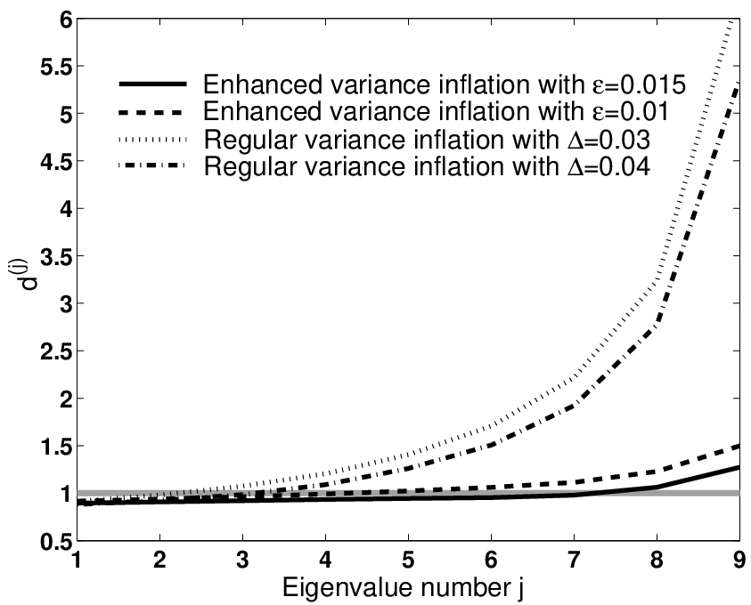
The second experiment was then repeated by using the regular variance inflation of Anderson and Anderson (1999) and Whitaker and Hamill (2002). In the regular variance inflation, all background ensemble perturbations are multiplied by , where is small, . This inflation strategy increases the total variance in the background ensemble by a factor of . It can be seen from Table 3 that, except for , the critical value of is less than half of the critical value of . The main difference between the two inflation schemes is that the enhanced scheme inflates the dominant eigendirections of the background covariance matrix less aggressively, and the least dominant eigendirections more aggressively. The numerical results suggest that this feature of the scheme is beneficial, indicating that the ensemble-based estimate of the background error is more reliable in the more unstable directions than in the other directions. This is also well illustrated by the quantitative results shown in Figure 7. To explain this figure, we define the true background error, by the difference between the truth, and the background mean, . We also define , the component of along the semi-axis of the probability ellipsoid, corresponding to the th largest eigenvalue, of , where . (The case is illustrated in Figure 8.) For an ensemble that correctly estimates the uncertainty in each basis direction, the time means of
| (89) |
should be close to one. When, for a given , the ratio is smaller than one, the ensemble tends to overestimate the distance between the truth and the background in the direction. When is larger than one, the ensemble underestimates this distance. Figure 7 shows that with the enhanced variance inflation the behavior of the ensemble is much better than with the regular variance inflation. This is especially true for the less dominant eigendirections, for which the ensemble with regular variance inflation significantly (by about a factor of 6) underestimates the distance between the truth and the mean background. We found that , the true background variance unexplained by the directions, , ; is about 3% of the true total variance () for all four cases shown in Figure 7. Thus the results indicate that the superior performance of the enhanced variance inflation is due to the better distribution of the variance between the resolved directions. We note that this advantage of the enhanced variance inflation could not be exploited if the analysis was not done in introduced in Section 2. Whether the advantage found for our enhanced variance inflation scheme carries over from the L96 model to a more realistic situation remains to be determined.
An interesting feature is the anomalously large error value of 0.29 at , in Table 3. An inspection of the data revealed that the higher time average is associated with a sudden and short-lived high amplitude spike in the rms analysis error. A further analysis of the problem revealed that spikes occur very rarely and they usually have small amplitude (smaller than 1). On rare occasions, however, the spikes can have large amplitude (sometimes larger than 5), and they can last a few thousand time steps. This phenomenon is illustrated by Figure 9, in which the first large spike occurs after more than 162,000 time steps (equivalent to about 104 years, assuming that one time step is equivalent to 6 hours) and lasts about 12,000 time steps (12 years in real time), and a second large spike develops 230,000 time steps (146 years in real time) later, which lasts for 3000 steps (2 years). The severity of this problem was studied by carrying out several long term integrations with different combinations of the tunable parameters. An interesting feature is that the spikes do not destroy the overall stability of the cycle; the large errors always disappear after a finite time and the mean error is smaller than 0.3. (For the case shown in Figure 9 the time mean error is 0.23). Spikes occur regardless of the size of the local region, and the type of the variance inflation scheme. They become less frequent, however, as the rank and the variance inflation are increased. In particular, no spikes were observed for . This suggests that the easiest way to prevent the occurrence of spikes is to choose a large enough variance inflation coefficient.
All results shown so far were obtained using (93) to generate the analysis ensemble, . This scheme results in analysis perturbations of the form as required by (34)-(36). In order to test the importance of including the small component, the first experiment was repeated by using solution 1 [(53)] for and instead of (36). (Using solution 1 and (36) would give the same result as (93) for our choice of .) This modified scheme, restricting the analysis perturbations to the dimensional space , is clearly inferior (compare Tables 2 and 4 and Tables 3 and 5). More precisely, the constrained scheme provides stable analysis cycles only if both and are relatively large. This is not unexpected, since setting the component to zero artificially reduces the total variance, . Increasing decreases the reduction in the total variance, while increasing compensates for an increasing part of the lost variance. Also, the constrained scheme is more stable when the enhanced variance inflation is used, indicating that correcting the distribution of the variance is not less important than increasing the total variance.
5.7 Discussion of the significance of the numerical experiments
Finally, we reemphasize that the significance of the results of all our numerical experiments on the toy model (87) is limited. Many important factors of real weather forecasting are not represented (e.g., model error), and very idealized conditions are assumed (e.g., known, normal, uncorrelated, unbiased, observation errors, and no “subgrid scale” stochastic-like input to the evolution of the “truth” state). On the other hand, it is also probably reasonable to assume that, if our assimilation procedure gave unfavorable results for our idealized toy model situation, then the scheme would also be unlikely to be effective in the real case. Thus, one can view the good results obtained with our assimilation scheme in these numerical experiments as necessary, but certainly not sufficient, for future successful performance in a real situation.
6 Summary and conclusions
In this paper, we have introduced a local method for assimilating atmospheric data to determine best-guess current atmospheric states. The main steps in our method are the following.
- •
The global analysis ensemble members are advanced by the atmospheric model to obtain the global background ensemble at the next analysis time.
- •
In each local region, each background ensemble member’s perturbation from the ensemble mean is used to construct a ‘local vector’.
- •
Each of the local vectors in the ensemble is projected onto the local low dimensional subspace.
- •
The observations are assimilated in each local region.
- •
The local analyses are used to determine the global analysis and an ensemble of global analysis states.
- •
The cycle is then repeated.
Numerical tests of the method using the Lorenz model, (87), have been performed. These tests indicate that the method is potentially very effective in assimilating data. Other potential favorable features of our method are that only low dimensional matrix operations are required, and that the analyses in each of the local regions are independent, suggesting the use of efficient parallel computation. These features should make possible fast data assimilation in operational settings. This is supported by preliminary work (not reported in this paper) in which we have implemented our method on the T62, 28-level version of the National Centers for Environmental Prediction Medium Range Forecasting Model (NCEP MRF). The assimilation of a total number of observations (including wind, temperature, and surface pressure observations) at and takes about 6 minutes CPU time on 40 2.8 GHz Xeon processors.
7 Acknowledgments
This work was supported by the W. M. Keck Foundation, a James S. McDonnell 21st Century Research Award, by the Office of Naval Research (Physics), by the Army Research Office, and by the National Science Foundation (Grants #0104087 and PHYS 0098632).
Appendix A: Global continuity of matrix square roots
Not all matrix square root definitions yield global continuity. One particular important mechanism for non-global-continuity of matrix square roots is that the eigenvectors of a globally continuous, symmetric, non-negative matrix, , may not be definable in a globally continuous manner. In particular, for smooth variation of in two dimensions, it can be shown that there will generically be isolated points in space where two of the eigenvalues of are equal. Following previous terminology in the field of quantum chaos (e.g., Ott 2002), we call such points “diabolical points” (e.g., Berry 1983). Assume that two eigenvalues of denoted and , are equal at the diabolical point , and denote their associated orthonormal eigenvectors by and . Now consider starting at a point and following a continuous path that encircles and returns to . Then it is shown in the paragraph below that, with continuous variation of and along the path, their directions are flipped by upon return to . This presents no contradiction, since orthonormal eigenvectors are arbitrary up to a change of sign, but it shows that a specific choice of and cannot be defined in a globally continuous manner. The positive symmetric square root ,
is globally continuous because returns to itself upon circuit around a diabolical point, even though may flip by . Thus the solutions for given in (53), (57), and (66) will be globally continuous, since positive symmetric square roots are used. The Cholesky square root will also yield global continuity. On the other hand, as an example of one of the choices that is unsatisfactory, the matrix square root choice,
is clearly not globally continuous if diabolical points are present.
In order to see how the above discussed property of diabolical points arises, consider the case of a two dimensional matrix,
| (90) |
The two eigenvalues of this matrix are
| (91) |
The eigenvalues are equal when the square root is zero, i.e., when and . These equations represent curves in the two-dimensional -space, and then, as illustrated in Figure 11a, equal eigenvalues generically occur at points of intersection of these curves (e.g. the point shown in the figure). It suffices to consider the neighborhood of such a diabolical point, and to use deformed coordinates in which and serve as axes (Figure 11b). Assume that we circuit around the origin of this system on the circular path of radius , shown in Figure 11b. Letting , , this path corresponds to continuous increase of from to . On this path one can show that
| (92) |
Thus the normalized eigenvector corresponding to is . As shown in Figure 11b, continuous increase of from point to point results in a flip in the orientation of . Thus (and similarly ) cannot be defined in a single-valued globally continuous manner.
Appendix B: obtained directly from
In this Appendix we show that as given by (85) can be used to directly obtain the analysis . In section 4.4, we discussed a variety of ways to compute a matrix to use in (45) to obtain, via (35), the analysis components, , in the low dimensional subspace . We now claim that (35), (36), (45), and (85) imply that
| (93) |
(The crucial difference between (93) and (45) is the absence of the superscribed circumflexes in (93)). Then in practice the columns of (93) can be used directly in (34). First we note that premultiplication of (93) by returns (45). Then further premultiplication by , together with (21), yields . This means that the projection of (93) onto agrees with (35). We verify (93) by showing that its projection into the complementary spaces and agree with the decomposition (35). It remains to show that the projection of (93) onto agrees with (35). Operating on both sides of (93) with and using in (85), we have
| (94) |
Now we recall from section 2 that and are constructed from spanning vectors that are eigenvectors of . Thus and are invariant under . Since (see equation 10), we have that commutes with the projection operators and . Thus
| (95) |
where the second equality follows because is in for any -dimensional column vector , thus yielding . From (94) and (95) we have or , as required by (36). This establishes (93). We find that use of (93) can be potentially advantageous for efficient parallel implementation of our method. We plan to further discuss this in a future publication applying our local ensemble Kalman filter to the operational global model of the National Centers for Environmental Prediction.
Appendix C: Enhanced Variance Inflation
In section 4.6 we mentioned the modification of or to prevent the occurrence of small eigenvalues in these matrices. Furthermore, we noted the possibility of an accompanying modification of the corresponding ensemble perturbations, so as to preserve the relation,
| (96) |
In the above equation we have suppressed the superscript or with the understanding that can apply to either the analysis or background.
We consider the example where is changed to a new covariance matrix by addition of a small perturbation in the form,
| (97) |
where denotes the unit matrix, and is the trace of ; i.e., it is the sum of its eigenvalues, and thus represents the total variance of the ensemble. (The case is illustrated in Figure 10.) Hence (97) increases the total variance by the factor , where we regard as small, . More importantly, for small , the additional variance represented in (97) results in a relatively small change in the largest eigenvalues of , but prevents any eigenvalue from dropping below (), thus effectively providing a floor on the variance in any eigendirection. Having modified to via (97), we now consider the modification of the ensemble perturbations, , to another set of ensemble perturbations, , with the perturbed covariance,
| (98) |
We use the result of sections 4.2 and 4.4 to choose the to minimize the difference with . This result is the same for all metrics that commute with (equivalently ). (Note that the solutions in (61) are all the same if , and commute.) Adopting this solution for , we introduce the orthogonal eigenvectors of , which we denote . The result for is then
| (99) |
where
| (100) |
with
| (101) |
and is the eigenvalue of corresponding to ; that is, .
Recalling that is diagonal (see (23)), we see that in the case (which is employed in section 5) the th component of the vector is . Consequently, for this case, (100) and (101) imply that is diagonal,
| (102) |
In the case , one could combine variance inflation and a procedure for obtaining the analysis ensemble (e.g., solutions 1, 2,, or 3 of section 4.2): First inflate ,
where is any chosen inflation; and, second, replace by in the chosen algorithm for determining the analysis ensemble.
References
Anderson, J. L., 2001: An ensemble adjustment filter for data assimilation. Mon. Wea. Rev., 129, 2884-2903.
Anderson, J. L., and S. L. Anderson, 1999: A Monte Carlo implementation of the nonlinear filtering problem to produce ensemble assimilations and forecasts. Mon. Wea. Rev., 127, 2741-2758.
Berry, M. V., 1983: Semiclassical mechanics of regular and irregular motion. In Chaotic Behavior of Deterministic Systems, R. H. G. Helleman and G. Ioos, eds., North-Holland, Amsterdam.
Bierman, G. J., 1977: Factorization Methods for Discrete Sequential Estimation. Mathematics in Science and Engineering, Academic Press, New York.
Bishop, C. H., B. J. Etherton, and S. Majumdar, 2001: Adaptive sampling with the Ensemble Transform Kalman Filter. Part I: Theoretical aspects. Mon. Wea. Rev., 129, 420-436.
Daley, R., 1991: Atmospheric data analysis. Cambridge University Press, New York.
Dee, D., S. Cohn, A. Dalcher, and M. Ghil, 1985: An efficient algorithm for estimating noise covariances in distributed systems. IEEE Trans. Automatic Control, 30, 1057-1065.
Evensen, G., 1994: Sequential data assimilation with a nonlinear quasi- geostrophic model using Monte Carlo methods to forecast error statistics. J. Geophys. Res., 99(C5), 10 143-10 162.
Evensen, G., and P. J. van Leeuwen, 1996: Assimilation of Geosat altimeter data for the Agulhas current using the ensemble Kalman Filter with a quasi-geostrophic model. Mon. Wea. Rev., 124, 85-96.
Fisher, M., 1998: Development of a simplified Kalman Filter. ECMWF Research Department Tech. Memo. 260, 16 pp. [Available from European Centre for Medium-Range Weather Forecasts, Shinfield Park, Reading, Berkshire, RG2 9AX, United Kingdom.]
Ghil, M., S. Cohn, J. Tavantzis, K. Bube, and E. Isaacson, 1981: Applications of estimation theory to numerical weather prediction. In Dynamic meteorology: data assimilation methods, L. Bengtsson, M. Ghil, and E. Kallen, eds. Springer-Verlag, New York, 139-224.
Hamill, T. M., and C. Snyder, 2000: A hybrid ensemble Kalman Filter-3D variational analysis scheme. Mon. Wea. Rev., 128, 2905-2919.
Hamill, T. M., J. Whitaker, and C. Snyder, 2001: Distance-dependent filtering of background error covariance estimates in an Ensemble Kalman Filter. Mon. Wea. Rev., 129, 2776-2790.
Houtekamer, P. L., and H. L. Mitchell, 2001: A sequential ensemble Kalman Filter for atmospheric data assimilation. Mon. Wea. Rev., 129, 796-811.
Houtekamer, P. L., and H. L. Mitchell, 1998: Data assimilation using an ensemble Kalman Filter technique. Mon. Wea. Rev., 126, 796-811.
Houtekamer, P. L., and H. L. Mitchell, 2001: A sequential ensemble Kalman Filter for atmospheric data assimilation. Mon. Wea. Rev., 129, 123-137.
Ide, K., P. Courtier, M. Ghil, and A. C. Lorenc, 1997: Unified notation for data assimilation: Operational, sequential, and variational. J. Meteor. Soc. Japan, 75(1B), 181-189.
Jones, R., 1965: An experiment in nonlinear prediction. J. Appl. Meteor., 4, 701-705.
Kalman, R., 1960: A new approach to linear filtering and prediction problems. Trans. ASME, Ser. D, J. Basic Eng., 82, 35-45.
Kalman, R., R. Bucy, 1961: New results in linear filtering and prediction theory. Trans. ASME, Ser. D, J. Basic Eng., 83, 95-108.
Kalnay, E., 2002: Atmospheric modeling, data assimilation, and predictability. Cambridge University Press, Cambridge, 341 pp.
Kalnay, E., and Z. Toth, 1994: Removing growing errors in the analysis. Preprints, 10th AMS Conference on Numerical Weather Prediction, Portland, OR, 212-215.
Keppenne, C., and H. Rienecker, 2002: Initial testing of a massively parallel ensemble Kalman Filter with the Poseidon Isopycnal Ocean General Circulation Model. Mon. Wea. Rev., 130, 2951-2965.
Lorenc, A., 1986: Analysis methods for numerical weather prediction. Quart. J. Roy. Meteor. Soc., 112, 1177-1194.
Lorenz, E. N., K. A Emanuel, 1998: Optimal sites for supplementary weather observations: Simulation with a small model. J. Atmos. Sci., 55, 399-414.
Lorenz, E. N., 1996: Predictability: A problem partly solved. Proc. Seminar on Predictability, Vol. 1, ECMWF, Reading, Berkshire, UK, 1-18.
Ott, E., 2002: Chaos in dynamical systems, (second edition). Cambridge University Press, Cambridge, chapter 11.
Patil, D. J., B. R. Hunt, E. Kalnay, J. A. Yorke, and E. Ott, 2001: Local low dimensionality of atmospheric dynamics. Phys. Rev. Lett., 86, 5878-5881.
Persson A., 2000: Synoptic-dynamic diagnosis of medium range weather forecast systems. Proceedings of the Seminars on Diagnosis of models and data assimilation systems. 6-10 September 1999, ECMWF, Reading, U.K., 123-137.
Petersen, D., 1973: A comparison of the performance of quasi-optimal and conventional objective analysis schemes. J. Appl. Meteor., 12, 1093-1101.
Szunyogh, I., Z. Toth, A. V. Zimin, S. J. Majumdar, and A. Persson, 2002: Propagation of the effect of targeted observations: The 2000 Winter Storm Reconnaissance Program. Mon. Wea. Rev., 130, 1144-1165.
Talagrand, O., 1981: A study of the dynamics of four-dimensional data assimilation. Tellus, 33, 43-60.
Tippett, M. K., J. L. Anderson, C. H. Bishop, T. M. Hamill, and J. S. Whitaker, 2002: Ensemble square-root filters. Mon. Wea. Rev., 131, 1485-1490.
Toth, Z., and E. Kalnay, 1993: Ensemble forecasting at NMC: The generation of perturbations. Bull. Amer. Meteorol. Soc., 74, 2317-2330.
Toth, Z., and E. Kalnay, 1997: Ensemble forecasting at NCEP and the breeding method. Mon. Wea. Rev., 127, 1374-1377.
Wang, X., and C. H. Bishop, 2002: A comparison of breeding and Ensemble Transform Kalman Filter ensemble forecast schemes. Preprints, Symposium on Observations, Data Assimilation, and Probabilistic Prediction, Orlando, FL., Amer. Meteor. Soc., J28-J31.
Whitaker, J. S., and T. H. Hamill, 2002: Ensemble Data Assimilation without perturbed observations. Mon. Wea. Rev., 130, 1913-1924.
Zimin A. V., I. Szunyogh, D. J. Patil, B. R. Hunt, and E. Ott, 2003: Extracting envelopes of Rossby wave packets. Mon. Wea. Rev., 131, 1011-1017.
Table Captions
Table 1. Dependence of the time mean rms error on the box size () and the rank () of the background covariance matrix. The symbol D stands for time mean rms errors larger than one, which is the rms mean of the observational errors. The coefficient of the enhanced variance inflation is .
Table 2. Dependence of the time mean rms error on the coefficient () of the enhanced variance inflation scheme and the rank () of the background covariance matrix. The meaning of D is the same as in Table 1. The window size is 13.
Table 3. Dependence of the rms analysis error on in the regular variance inflation scheme and the rank () of the background error covariance matrix. The meaning of D is the same as in Table 1. The window size is 13.
Table 4. Same as Table 2 except that Solution 1 and is used (instead of 93) to obtain the analysis ensemble.
Table 5. Same as Table 3 except that Solution 1 and is used (instead of 93) to obtain the analysis ensemble.
Figure Captions
New Figure 1.
Illustration of the Local Ensemble Kalman Filter scheme as given by the six steps listed in the introduction. The symbols in the figure are as follows:
- •
= the analysis ensemble fields as a function of position on the globe at time .
- •
= ensemble of background atmospheric state in local region .
- •
= the local low dimensional subspace in region .
- •
= the mean analysis state in .
- •
= the analysis error covariance matrix in .
Figure 1. Probability ellipsoid for .
Figure 2. Illustration of the local region with a central region .
Figure 3. The rms error of the full Kalman filter as function of the number of ensemble members. Shown are the results for (solid line), (dashed line), and (dotted-dashed line).
Figure 4. The rms error of the local ensemble Kalman filter as function of the number of ensemble members. Shown are the results for (solid line), (dashed line), and (dotted-dashed line).
Figure 5. The rms error of the different analysis schemes as function of the number of observations. Shown are the results for the full Kalman filter [4% variance inflation] (dashed line), conventional scheme (dashed-dotted line), direct insertion (solid line with diamonds), and the local ensemble Kalman filter [3% variance inflation] (solid line).
Figure 6. The ratio at as function of for two different values of and .
Figure 7. Projection of the true background error, , on the main axes of the probability ellipsoid.
Figure 8. The long time evolution of the rms analysis error for a set of parameters that allow spikes to occur.
Figure 9. The effect of the enhanced variance inflation (equation 97) on the probability ellipsoid. For the case , and .
Figure 10. (a) The curves and cross at a diabolical point . (b) The eigenvector flips by on one circuit around the diabolical point.
| 3 | 4 | 5 | 6 | 7 | 8 | 9 | ||
|---|---|---|---|---|---|---|---|---|
| 5 | 0.24 | 0.23 | ||||||
| 7 | 0.22 | 0.22 | 0.21 | 0.22 | ||||
| 9 | 0.22 | 0.21 | 0.21 | 0.21 | 0.21 | 0.21 | ||
| 11 | D | D | 0.20 | 0.20 | 0.20 | 0.20 | 0.20 | |
| 13 | D | D | 0.20 | 0.20 | 0.20 | 0.20 | 0.20 | |
| 15 | D | D | D | 0.22 | 0.20 | 0.2 | 0.20 |
| 4 | 5 | 6 | 7 | 8 | 9 | ||
|---|---|---|---|---|---|---|---|
| 0.008 | D | D | 0.44 | 0.20 | 0.20 | 0.20 | |
| 0.010 | D | D | 0.2 | 0.2 | 0.20 | 0.20 | |
| 0.012 | D | 0.20 | 0.20 | 0.20 | 0.20 | 0.20 | |
| 0.014 | D | 0.20 | 0.20 | 0.20 | 0.20 | 0.20 | |
| 0.016 | D | 0.20 | 0.20 | 0.20 | 0.20 | 0.20 | |
| 0.018 | D | 0.20 | 0.20 | 0.20 | 0.20 | 0.20 | |
| 0.020 | 0.21 | 0.20 | 0.20 | 0.20 | 0.20 | 0.20 |
| 4 | 5 | 6 | 7 | 8 | 9 | ||
|---|---|---|---|---|---|---|---|
| 0.020 | D | D | 0.50 | 0.30 | D | D | |
| 0.024 | D | 0.87 | 0.42 | 0.21 | 0.21 | 0.21 | |
| 0.028 | 0.21 | 0.36 | 0.20 | 0.20 | 0.20 | 0.20 | |
| 0.032 | 0.20 | 0.20 | 0.20 | 0.20 | 0.20 | 0.20 | |
| 0.036 | 0.20 | 0.20 | 0.20 | 0.20 | 0.29 | 0.20 | |
| 0.040 | 0.20 | 0.20 | 0.20 | 0.20 | 0.20 | 0.20 | |
| 0.044 | 0.20 | 0.20 | 0.20 | 0.20 | 0.20 | 0.20 | |
| 0.048 | 0.20 | 0.20 | 0.20 | 0.20 | 0.20 | 0.20 |
| 4 | 5 | 6 | 7 | 8 | 9 | ||
|---|---|---|---|---|---|---|---|
| inflation coefficient | |||||||
| 0.010 | D | D | D | 0.41 | 0.20 | 0.20 | |
| 0.012 | D | D | D | 0.27 | 0.20 | 0.20 | |
| 0.014 | D | D | D | 0.21 | 0.20 | 0.20 | |
| 0.016 | D | D | D | 0.21 | 0.20 | 0.20 | |
| 0.018 | D | D | 0.46 | 0.21 | 0.20 | 0.20 | |
| 0.020 | D | D | 0.28 | 0.21 | 0.20 | 0.20 | |
| 0.022 | D | D | 0.23 | 0.21 | 0.20 | 0.21 | |
| 0.024 | D | D | 0.22 | 0.21 | 0.21 | 0.21 |
| k | 4 | 5 | 6 | 7 | 8 | 9 | |
|---|---|---|---|---|---|---|---|
| 0.020 | D | D | D | D | D | D | |
| 0.024 | D | D | D | D | 0.75 | 0.21 | |
| 0.028 | D | D | D | D | 0.22 | 0.21 | |
| 0.032 | D | D | D | D | D | 0.20 | |
| 0.036 | D | D | D | D | 0.21 | 0.25 | |
| 0.040 | D | D | D | 0.22 | 0.21 | 0.20 | |
| 0.044 | D | D | D | D | 0.20 | 0.20 | |
| 0.048 | D | D | D | 0.25 | 0.20 | 0.20 |

The symbols in the figure are as follows:
- •
= the analysis ensemble fields as a function of position on the globe at time .
- •
= ensemble of background atmospheric state in local region .
- •
= the local low dimensional subspace in region .
- •
= the mean analysis state in .
- •
= the analysis error covariance matrix in .