Long range correlations in DNA sequences
Abstract
The so called long range correlation properties of DNA sequences are studied using the variance analyses of the density distribution of a single or a group of nucleotides in a model independent way. This new method which was suggested earlier has been applied to extract slope parameters that characterize the correlation properties for several intron containing and intron less DNA sequences. An important aspect of all the DNA sequences is the properties of complimentarity by virtue of which any two complimentary distributions (like is complimentary to or is complimentary to ) have identical fluctuations at all scales although their distribution functions need not be identical. Due to this complimentarity, the famous DNA walk representation whose statistical interpretation is still unresolved is shown to be a special case of the present formalism with a density distribution corresponding to a purine or a pyrimidine group. Another interesting aspect of most of the DNA sequences is that the factorial moments as a function of length exceed unity around a region where the variance versus length in a log-log plot shows a bending. This is a pure phenomenological observation which is found for several DNA sequences with a few exception. Therefore, this length scale has been used as an approximate measure to exclude the bending regions from the slope analyses. The asymmetries in the nucleotide contents or the patchy structure as a possible origin of the long range correlations has also been investigated.
pacs
PAC(s) 87.14.Gg.87.16.AC,05.10.-aI INTRODUCTION
Recently, there has been considerable interest in the finding of long range correlations in genomic DNA sequences [1]. A DNA sequence is a chain of sites, each occupied by either a purine (Adenine and Guanine) or a pyrimidine (Cytocyine and Thymine) group. For mathematical modeling, the DNA sequence might be considered as a string of symbols (G, A, T and C) whose correlation structure can be characterized completely by all possible base-base correlation functions or their corresponding power spectra. Different techniques including mutual information functions and power spectra analyses [1, 2, 3, 4, 5, 6, 7, 8, 9], auto correlation [10, 11, 12], DNA walk representation [13, 14, 15, 16, 17, 18, 19, 20], wavelet analysis [21, 22] and Zipf analysis [23] were used for statistical analyses of DNA sequences. But despite the effort spent, it is still an open question whether the long range correlation properties are different for protein coding (exonic) and non coding (intronic, intergenemic) sequences [24]. One more fundamental ground, there is still continuing debate as to whether the reported long range correlations really mean a lack of independence at long distances or simply reflect the patchiness (bias in nucleotide composition) of DNA sequences. There have been attempts to eliminate local patchiness using methods such as min-max [13], detrended fluctuation analysis (DFA) [24, 25] and wavelet analysis [21]. In spite of its success in modeling the long range correlations observed in DNA sequences, as indicated by the power law increase in the variance and the inverse power law spectrum [5, 9], the problem of the correct statistical interpretation of DNA walk is still unresolved and is attracting the attention of an increasing number of investigators. Since approaches based on different models predict different correlation structure, there is no unique measure of the degree of correlation in DNA sequences. Therefore, it is very important to investigate the correlations and extract the power law exponent rather in a model independent way so that the interpretation of the data including the theoretical analysis becomes more meaningful. There is another confusion related to this study is the absence of a clear definition of the term ”long range”. Clearly, what is considered to be long is relative to what is considered to be short. To over come some of these problems, recently we have suggested a new method [26] to measure the degree of correlations using the variance analysis of the density distribution of a single or a group of nucleotides. We have also suggested a way to find out an approximate length scale above which all DNA sequences show strong long range correlations irrespective of their intron contents while below this, the correlation is relatively weak. Further, the density distribution which is nearly Gaussian at short distances shows significant deviations from the Gaussian statistics at large distances. In this paper, we present the details of the analyses and also extract the correlation parameter for several intron containing and intronless sequences.
II Density distribution and Factorial moments:
In the present method, we build the frequency spectrum of a single or a group of nucleotides by dividing the DNA sequence into many equal intervals of length . For example, to build a purine spectrum, we compute
| (1) |
where =1 if the site is occupied by a G or A and =0 otherwise. Ideally, one can divide the entire DNA sequence of length into equal intervals of size . The purine or GA spectrum can be built by computing from all the intervals. Alternatively, can be computed in any segment between and and the spectrum ( distribution or ) is built by varying the starting position from 1, 2, 3 etc upto so as to cover the whole sequence 11 1 At short distances, can be zero due to the non occurence of a given nucleotide. In such cases, the density spectrum can be built either including or excluding zeroth channel. In this analysis, we include zeroth channel also so that the complementarity is satisfied which is unlike the case when the zeroth channel is excluded. See appendix B for details. We adopt this second procedure for better statistics. Finally, the standard deviation (SD) of this distribution can be obtained from which in general will depend on the interval or the window size .
In addition to the standard deviation , we also compute the factorial moments ’s of . The normalized factorial moments of order q are written as
| (2) |
where
| (3) |
As will be shown later, the factorial moment has the distinct advantage over the normal moments in identifying the genomic sequence from the random one. It may be mentioned here that for random Poisson distribution, the factorial moments for all q’s become unity i.e. for
| (4) |
the above factor for becomes
| (5) |
which gives =1.
In this work, we have applied the above factorial moment analysis (generally used to study the fluctuations during a phase transition [27]) to study the dynamical fluctuations present in the DNA sequences.
III Principle of complimentarity
A general property noticed for all the genomic sequences (of statistically significant length) with a few exceptions is that the distributions of any single or group of nucleotides which has a probability of occurrence has the same variance as that of its complimentary group that has the probability of occurrence , although both have different distribution functions. This would imply that even a single nucleotide distribution say distribution will have same variance as that of distribution or a distribution will have identical variance as that of distribution. Figure 1 shows versus plots for and distributions (solid curves) for two typical sequences of (Drosphilia Melanogaster, MHC, 22663 bps, , , , ) and (yeast mitochondrial DNA, , , , ). As can be seen from the figure, the and distributions have same at all scale as that of and distributions (filled circles) although the distribution functions of the two complimentary groups need not be identical. The above agreement is exact for most of the DNA sequences (with a few exceptions) as well as for the random sequences. For example, the for and distributions of and ( with a mobile transposion (9147 bps) at location 22000 bps) show to deviations at all scale depending on the total length of the sequences where as for other DNA as well as random sequences, this agreement is exact. (This difference is not visible from figure 1 in case of as the deviation is insignificant over a large distance).

Within the present formalism, we can also reproduce the result of random walk model (See appendix for more detail) by assigning for purine group ( and ) and for pyrimidine group ( and ). However, unlike the random walk model of interpreting and as the probability of step up and step down, can be considered as the frequency distribution of which gives the excess or deficit of purines over pyrimidines. The versus as obtained from this assignment has also been shown in figure 1 (see the dotted curves labeled ) for comparison. It is interesting to note that the curves shows a parallel shift with respect to the or curves indicating that or distributions and model have similar fluctuations at all scale. This is an interesting observations, as we can now use or distributions as alternatives to the DNA walk representation to study the correlation. The advantage is, since represents a sum, unlike the DNA walk model, the entire spectrum lies to the positive side of the coordinates which is essential to compute various higher moments like of the distributions.
It is also important to note that although the complimentary distributions have same at all scale, the distribution functions need not be exactly identical. Figure 2 shows a typical normalized density distribution functions of two complimentary distributions and for the above two sequences ( and ) as a function of (where is the average count ) at a typical length scale of (figures in left). The figures to the right shows distributions (-axis is shifted by 100 for clarity) corresponding to the two purely random sequences having same length and nucleotide contents as that of and sequences. It is interesting to note that although versus plots are (nearly) identical , both distributions have same fluctuations at all scales, the distribution functions are not identical. This is an important characteristic of a DNA sequence which is not found in case of a random one.

IV Extraction of slope parameter
The long range correlations are generally studied from the relation where the parameter is extracted from the versus plot in the log-log scale. For the case of a completely random sequence, . The deviation of from indicates presence of long range correlations. We have estimated of , , , and distributions for several DNA sequences and found that versus plot in the log-log scale is not linear over the entire length 22 2 We consider only the , , and distributions to extract the correlation parameters for the individual nucelotides and distributions to simulate the results of random walk model. Figure 3 shows versus plot (bottom panel) for a typical sequence of length Mbps (solid curves) and Kbps (dotted curves) respectively. The top panel shows the factorial distributions of =2, 3, 4 and 6 for a typical distributions, although similar plots can be obtained for other nucleotide distributions as well. A general feature of the factorial moments of the DNA sequence with a few exception is that at short distances, for all and exceeds unity at some point say at . This behavior is not found in case of a purely random sequence where is always . Further, all ’s do not cross unity exactly at the same point, being more for higher values. However, this variation is insignificant over a very large scale if we restrict to some of the lower moments say up to .
From these plots and also from the several other studies, we make following few observations; (i) The versus plot is not linear through out, rather starts bending around some region (say , which could be different for different distributions) indicating a change of slope from to , (ii) For most of the cases, while shows weak deviation from , deviates significantly from and also depends on the sequence length , (iii) The individual nucleotide distributions may have stronger correlations than any sum like and distributions or any other combinations.

Since versus in the log-log plot starts bending around , we can extract the slope by dividing the entire length into two segments; one for and the other one for . This can be done by examining each case individually. However, we have noticed an approximate correlation between this bending region in versus plot and the cross over points of the corresponding factorial moments i.e. the slope changes around the same region where the factorial moments become unity. This is a pure phenomenological observation which is found for several DNA sequences as listed in tables with a few exceptions which we will discuss below. It may be mentioned here that although, the two complimentary distributions have same fluctuations, both need not have identical factorial moments. Figure 4 shows the plots of versus for and distribution for a sequence. Since both are complimentary, they have identical fluctuations at all scales (hence same bending region), but the cross over regions in plots are different, being higher for distributions (due to large average values at all scales). While the value of the distribution shows an approximate correlation with the bending region of versus plot where a possible slope change occurs, the values of distribution has no such correlations. This is true for any complementary distributions of , , and except for and distributions since both have nearly same overlapping cross over regions.

Therefore, only the values of the , , , and distributions are used as an approximate length scales . The entire length of the sequence is divided into two parts one for and other for where and are the minimum and maximum of all the corresponding to , , , and distributions. The , i.e. we have at least independent data sets so that the statistical analysis becomes meaningful. Therefore, excluding the region , we have extracted and since the linearity in these two segments are found to be extremely good for most of the cases. The results are summarized in three tables which covers both intronless and intron containing sequences. The table shows the length of the sequence used in the analyses, the cross over values ( same as ), the slope parameters and and also the corresponding percentage of the nucleotide contents . A general observation is that the sequence is weakly correlated at short distance with which is quite close to where as for , the correlation is relatively stronger with a larger value of . Now we discuss a few exceptions like in the case of and ( bacteriophage, bps). Figure 5 shows the factorial moments of a typical distributions. In both the cases, the factorial moments do not have any cross over point. In case of , the factorial moments are much higher than unity even at small distance and starts decreasing afterwards. The similar behavior is found for distribution also. However, the , and distributions do have points. Therefore, using as and , we estimated and for , , , and distributions which are listed in table III. The symbol indicates absence of any critical value. It is interesting to note that is quite large and in some cases . On the other hand , the factorial moments of the sequence like do not reach unity at any scale. The absence of such type of scale has been indicated by the symbol in table III. This type of sequences behave like a pure random one having values quite close to . We have listed a few such sequences with exceptions in table III.

Further, we would like to mention here that we have noticed that the factorial moments for many sequences starts decreasing at large distances. Also for a few cases, the factorial moments start decreasing even at a very short distances. Consequently, the slope also changes accordingly. However, we would not like to assign any reasons due to lack of enough statistics.
The slope with corresponds to the case of a normal diffusion process of a random Brownian trajectory. The basic idea of a Brownian motion is that of a random walk having a Gaussian distribution probability for the position of the random walker after a time with the variance () proportional to ( where ). This corresponds to the case of normal diffusion. However, nature shows enough examples of anomalous diffusion characterized by a variance which does not follow a linear growth in time [28]. In such cases either the diffusion is accelerated if or the growth is dispersive if . As found in the analyses (see tables I and II), at large distances for most of the sequences irrespective of their intron contents. However, a few sequences as shown in table III, not only peculiar, may also have which decreases at large distances. In such cases, which may indicate the influence of dispersive dynamics. This aspect needs further investigations. Finally, we would like to add here that is close to for most of the sequences at short distance (see tables I and II). Although, would imply about a random behavior, it can not be told conclusively from the present analyses unless the short distance effects are taken into consideration [29].
V Patchy sequences
In the following, we investigate whether the mosaic character of DNA consisting of patches of different composition can account for apparent long range correlations in DNA sequences[18]. The Chargaff’s second parity rule states that in a single strand and . However, asymmetries in base composition have been observed in many sequences. A quantitative estimate of the and skews can be obtained from the relation (Excess of nucleotides over nucleotides) and (Excess of nucleotides over nucleotides). This is, operationally equivalent to estimating as defined in Eq.(1) except now represents the count for skew and for skew in a fixed window size of . We consider as an example and plot (defined appropriately) versus where the starting position of the sliding window varies from , , etc upto . Figure 6 shows the plots of and skews as a function of the length for a typical sequence. The plots show a change in the direction of the slope with a change in sign of the skew. The quantity and quality of the skew can be assessed from the or from the inverted- shape of the curves.
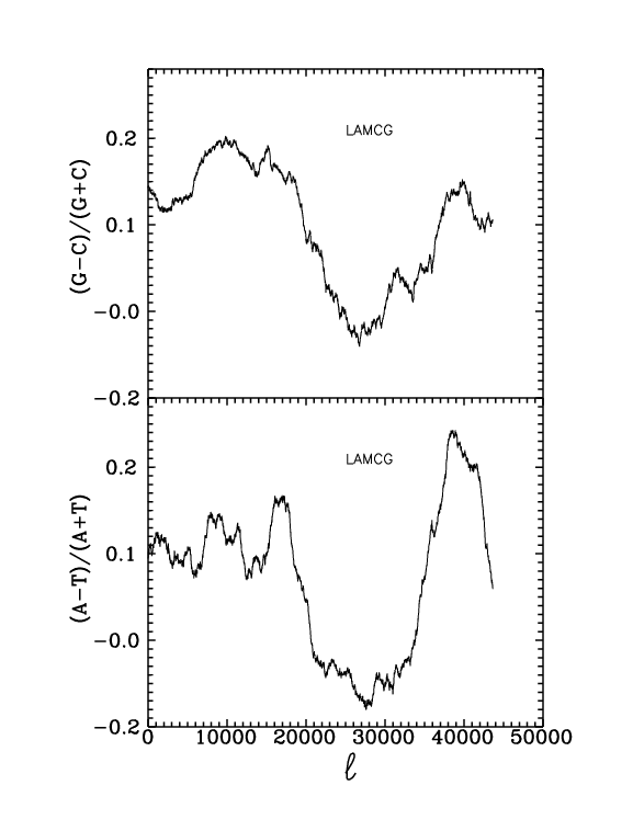
From the above plots, we can identify three well known compositional domains of of size 22000 bps ( contents 0.54), 17000 bps ( contents 0.47) and 9000 bps ( contents 0.54). We also consider an artificially generated sequence by joining three random patches of size 22000 bps, 17000 bps and 9000 bps respectively with appropriate , , and contents. We also consider another heterogeneous sequence generated from DNA by a mobile insertion of TN10 at location 22000 bps. The corresponding random patches are of size 22000 bps, 9147 bps and 22000 bps respectively 33 3 Please note the distinction between the random sequence which is generated by joining three random patches of total length and a pure random one of length . Although, both the sequence has same percentage of nucleotide contents in the length , the former is random only patch wise.

Figure 7 shows the versus plot of a typical distribution for and for an artificially generated sequence (random only patch wise). Interestingly, the factorial moments for both the cases behave similarly. Figure 8 shows a similar versus plot both for real and artificially generated (from random patches) sequences. Although, in some cases both agree, in general they are not identical at the individual nucleotide levels particularly at large distances (Note that the scale is highly compressed). This deviation would mean that at large distances, the density distribution functions will have significant discrepancy due to different widths. So at a first look from the versus plot, we can say that the actual DNA sequences and the RANDOM patches need not have identical slopes (hence the width ) at large distances for all the nucelotides although they agree in some cases. Even at short distances, although the DNA and the RANDOM sequences have nearly identical width , the full shape of the distributions need not be identical. To demonstrate this, we invoke the principle of complimentary which was mentioned before.

Figure 9(a) shows a and distribution (left most) for a sequence at . Notice that although versus plots are identical, i.e. both distributions have same fluctuations at all scales, the distribution functions are not same. Such differences are not found for a real random sequence (right most). The middle figure corresponds to the case of artificially generated random sequence. Although, the artificially generated sequence mimics the real sequence to some extent, it is not fully capable of reproducing the characteristic of a real sequence. Figure 9(b) shows another comparison for a sequence for and distributions. This discrepancy will be more prominent at higher values which the artificially generated sequence can not reproduce.

VI Density distributions
In [26], we had demonstrated that the density distribution is Gaussian at short distances and starts deviating from it as the distance increases. Figure 10 shows another example where has been plotted for two complimentary distributions at , and respectively. The complimentary distributions are nearly identical at short distance and coincide with the random distributions where as distributions for , and pure random one are all different at larger distances.

Thus, irrespective of intron contents, most of the sequences follow Gaussian statistics at short distances. However, at large distances, the statistics deviates significantly from the Gaussian nature.
VII Conclusions
In conclusion, we have extended our previous work to extract the slope parameter for several intron containing and intron less DNA sequences. The advantage of the present method is that the variance analysis can be applied to any individual or group of nucleotides. We believe that the individual nucleotides provide a more fundamental measure of the correlation than any combination or group (like the DNA walk representation) where the effects may get reduced or washed out. Another interesting aspect is the (lower) factorial moments of most of the DNA sequences cross unity in a very narrow region in where the versus plot in the log-log scale also shows a bending. Although, a formal justification to this correlation has not been provided, we have used this scale as an approximate measure to exclude the bending regions from the slope analyses. Based on this scale, we divide the DNA sequence into two segments to extract the slope parameters. It is found that below this scale, the correlation is weak and the DNA statistics is essentially Gaussian while above this all DNA sequences show strong long range correlations irrespective of their intron contents with a significant deviation from the Gaussian behavior. It may be mentioned here that the controversies that exist in this field of research are primarily due to different approaches that are adopted in various models. In this context, our analyses is model independent as it only involves the counting of an individual or a group of nucleotides in a given length to build the density distribution. In this work, we do not advocate for any specific model, although the extracted slope parameters indicate the presence of anomalous diffusion of both enhanced and dispersive nature. Instead, we provide an elegant tool to measure the degree of correlations unambiguously so that the interpretation of the data including theoretical analyses will become more meaningful. This work will also provide further impetus to develop models for the understanding of the DNA dynamics.
| Sequence | L | , | G | A | T | C | GA |
|---|---|---|---|---|---|---|---|
| Human -globin | 73,308 | 12 | 14 | 14 | 14 | 32 | |
| (Chromosomal region) | 0.640 | 0.644 | 0.671 | 0.620 | 0.652 | ||
| HUMHBB | 0.703 | 0.783 | 0.812 | 0.655 | 0.758 | ||
| P | 20.2 | 30.1 | 30.4 | 19.3 | 50.3 | ||
| Adenovirus type 2 | 35,937 | 24 | 12 | 12 | 36 | 132 | |
| (Intron containing) | 0.598 | 0.586 | 0.567 | 0.583 | 0.564 | ||
| ADRCG | 0.862 | 0.815 | 0.816 | 0.758 | 0.661 | ||
| P | 27.3 | 23.2 | 21.6 | 27.9 | 50.5 | ||
| Chicken embryonic MHC | 31,111 | 24 | 36 | 14 | 28 | 48 | |
| (Gene) | 0.644 | 0.578 | 0.658 | 0.581 | 0.623 | ||
| CHKMYHE | 0.775 | 0.698 | 0.800 | 0.715 | 0.762 | ||
| P | 22.2 | 31.3 | 26.7 | 19.8 | 53.5 | ||
| Human -cardiac MHC | 28,438 | 16 | 16 | 10 | 18 | 20 | |
| (Gene) | 0.638 | 0.579 | 0.627 | 0.620 | 0.664 | ||
| HUMBMYH7 | 0.681 | 0.663 | 0.700 | 0.673 | 0.688 | ||
| P | 25.9 | 23.6 | 23.0 | 27.5 | 49.5 | ||
| Drosophila melanogaster MHC | 22,663 | 20 | 20 | 14 | 36 | 156 | |
| (Gene) | 0.648 | 0.594 | 0.644 | 0.562 | 0.569 | ||
| DROMHC | 0.820 | 0.652 | 0.798 | 0.707 | 0.719 | ||
| P | 20.5 | 30.3 | 25.4 | 23.8 | 50.8 | ||
| Chicken c-myb oncogene | 8200 | 14 | 10 | 10 | 12 | 48 | |
| (Gene) | 0.663 | 0.661 | 0.688 | 0.670 | 0.645 | ||
| CHKMYB15 | 0.749 | 0.873 | 0.752 | 0.852 | 0.550 | ||
| P | 28.4 | 21.9 | 23.5 | 22.2 | 50.3 |
| Sequence | L | , | G | A | T | C | GA |
|---|---|---|---|---|---|---|---|
| 1200000 | 100 | 32 | 32 | 92 | 684 | ||
| 0.535 | 0.542 | 0.549 | 0.532 | 0.529 | |||
| 0.665 | 0.639 | 0.664 | 0.674 | 0.614 | |||
| 0.654 | 0.654 | 0.655 | 0.715 | 0.563 | |||
| P | 27.2 | 23.6 | 24.2 | 25.0 | 50.8 | ||
| H. Influenzae | 240000 | 52 | 48 | 56 | 52 | 214 | |
| 0.542 | 0.552 | 0.543 | 0.547 | 0.543 | |||
| 0.720 | 0.712 | 0.635 | 0.770 | 0.709 | |||
| P | 17.9 | 31.6 | 30.7 | 19.8 | 49.5 | ||
| Bacillus subtilis | 3840x60 | 80 | 40 | 22 | 132 | 274 | |
| 0.538 | 0.545 | 0.550 | 0.508 | 0.536 | |||
| 0.815 | 0.770 | 0.816 | 0.779 | 0.766 | |||
| P | 24.5 | 29.5 | 26.5 | 19.5 | 54.0 | ||
| Mycobacterium | 9665x60 | 20 | 64 | 44 | 24 | 136 | |
| tuberculosis | 0.549 | 0.535 | 0.548 | 0.540 | 0.542 | ||
| 0.827 | 0.681 | 0.826 | 0.765 | 0.791 | |||
| P | 15.92 | 34.57 | 33.73 | 15.78 | 50.49 | ||
| Cyano bacterium | 4166x60 | 32 | 40 | 28 | 24 | 304 | |
| 0.545 | 0.532 | 0.542 | 0.541 | 0.535 | |||
| 0.730 | 0.678 | 0.763 | 0.733 | 0.587 | |||
| P | 24.1 | 26.0 | 26.0 | 23.9 | 50.1 | ||
| Schizosaccharomyces | 19431 | 32 | 60 | 80 | 304 | 160 | |
| Mitochondiron | 0.547 | 0.561 | 0.568 | 0.504 | 0.543 | ||
| NC-001326 | 0.698 | 0.690 | 0.774 | 0.465 | 0.773 | ||
| P | 15.8 | 33.8 | 36.1 | 14.3 | 49.6 | ||
| Human Cytomegalovirus | 229354 | 36 | 10 | 10 | 32 | 148 | |
| Strain AD169 | 0.582 | 0.588 | 0.596 | 0.581 | 0.575 | ||
| HEHCMVCG | 0.806 | 0.799 | 0.800 | 0.800 | 0.682 | ||
| dmal | 889x60 | 20 | 12 | 12 | 22 | 68 | |
| 0.575 | 0.628 | 0.599 | 0.559 | 0.60 | |||
| 0.730 | 0.782 | 0.602 | 0.720 | 0.596 | |||
| Chicken nonmuscle MHC | 7003 | 96 | 72 | 12 | 28 | 64 | |
| (cDNA) | 0.573 | 0.538 | 0.569 | 0.554 | 0.627 | ||
| CHKMYHN | 0.722 | 0.833 | 0.841 | 0.601 | 0.842 | ||
| P | 27.0 | 31.2 | 20.6 | 21.2 | 58.2 | ||
| Bacteriophage | 48,502 | 56 | 36 | 18 | 124 | 168 | |
| (Intronless virus) | 0.563 | 0.541 | 0.598 | 0.513 | 0.550 | ||
| LAMCG | 0.935 | 0.819 | 0.911 | 0.810 | 0.866 | ||
| P | 26.4 | 25.4 | 24.7 | 23.5 | 51.8 | ||
| Human dystrophin | 13,957 | 136 | 56 | 14 | 22 | 128 | |
| (cDNA) | 0.530 | 0.552 | 0.569 | 0.552 | 0.544 | ||
| HUMDYS:M18533 | 0.738 | 0.634 | 0.777 | 0.720 | 0.725 | ||
| P | 22.4 | 33.0 | 24.7 | 19.9 | 55.4 |
| Sequence | L | , | G | A | T | C | GA |
|---|---|---|---|---|---|---|---|
| SC-MIT | 85779 | * | 36 | 36 | * | 184 | |
| Nc-001224 | 0.732 | 0.697 | 0.680 | 0.720 | 0.578 | ||
| 0.698 | 0.540 | 0.747 | 0.508 | 0.730 | |||
| P | 9.1 | 42.2 | 40.7 | 8.0 | 51.3 | ||
| Pichia canadensis | 27694 | * | 36 | 64 | * | 96 | |
| Mitochondiron | 0.654 | 0.688 | 0.624 | 0.615 | 0.620 | ||
| NC-001762 | 0.662 | 0.755 | 0.784 | 0.660 | 0.801 | ||
| P | 10.2 | 41.6 | 40.2 | 8.0 | 51.84 | ||
| Ti(Plasmid) | 24595 | 76 | 24 | 32 | 40 | - | |
| 0.543 | 0.564 | 0.552 | 0.586 | 0.508 | |||
| 0.706 | .700 | 0.676 | 0.728 | 0.433 | |||
| P | 23.5 | 26.6 | 27.5 | 22.4 | 50.1 | ||
| BacteriophageT7 | 39937 | - | 116 | 884 | 1284 | - | |
| NC-001604 | 0.526 | 0.571 | 0.529 | 0.530 | 0.530 | ||
| 0.560 | 0.587 | 0.590 | 0.566 | 0.551 | |||
| P | 25.8 | 27.2 | 24.4 | 22.6 | 53.0 | ||
| Tyorg | 196x60 | - | 96 | - | 36 | 96 | |
| 0.491 | 0.560 | 0.515 | 0.620 | 0.587 | |||
| 0.370 | 0.715 | 0.514 | 0.799 | 0.704 | |||
| P | 16.0 | 35.9 | 26.7 | 21.4 | 51.9 |
Random walk model
The method of DNA walks, first suggested by Peng et al [13] is based on the rule that the walker either moves up or down for each step of the walk. This is the case of a correlated random walk and differs from an uncorrelated walk where the direction of each step is independent of the previous steps. Further they assign if a pyrimidine occurs at the site whereas if the site contains a purine. The net displacement of the walker after steps is defined as
| (6) |
The standard deviation of the above quantity can be estimated from
| (7) |
where is the number of nucleotides in the entire sequence and
| (8) |
where . It was found [13] that the fluctuations can be approximated by
| (9) |
where is the correlation exponents. For close to , there is no correlation or only short range correlation in the sequence. If is significantly different from , it indicates long range correlations.
B
In the previos analyses, we account for the non-occurence of a particular nucleotide. This is operationally equivalent to building the density spectrum including . If the nucleotide compositional asymmetry is quite large like , the occurence can be zero for some nucleotides particularly at short distances. Therefore, we can build distribution either including or excluding zeroth channel. The figure B1(a) shows the comparison of versus plot for two complimentary distributions corresponding to a sequence both with (top panel where and distributions have identical slopes at all scales) and without (bottom panel) inclusion of channel in the spectra. Interestingly, absence of channel does not satisfy the complimentarity relation particularly at short distances. However, the difference does not exist at larger distances where always . Figure B1(b) shows another example of versus plot for a typical sequence. The spectrum with exclusion of channel behaves differently when zeroth channel is included (compare it with figure 5 where versus has no cross over).

Since the spectrum behaves differently when zeroth channel is not included, we have analysed the spectrum of three typical sequences listed in the table below. Notice now that while values are essentially same as before, the values are quite different. In fact, we have noticed a general trend where is higer than the previous values although the corresponding density distributions do not deviate significantly from the Gaussian behavior at short distances. However, in the previous analysis, we alwyas include the zeroth channel so that the complimentarity properties is satisfied at all scales. Moreover, we also found a correlation between and Gaussian statistics, namely the deviation of from also shows a corresponding deviation of distribution from Gaussian behavior. For example, in case of , the is quite large at a short distance. Accordingly, the distribution also shows strong deviation from the Gaussian statistics. However, this is not necessarilly true when complimentarity is not preserved while building the spectrum. At short distances, the deviation of from does not always mean a strong deviation from the Gaussian statistics.
| Sequence | L | , | G | A | T | C | GA |
|---|---|---|---|---|---|---|---|
| Bacteriophage | 48,502 | 56 | 36 | 18 | 124 | 168 | |
| (Intronless virus) | 0.720 | 0.670 | 0.740 | 0.680 | 0.580 | ||
| LAMCG | 0.935 | 0.819 | 0.910 | 0.800 | 0.860 | ||
| P | 26.4 | 25.4 | 24.7 | 23.5 | 51.8 | ||
| SC-MIT | 85779 | 14 | 36 | 40 | 12 | 184 | |
| Nc-001224 | 0.703 | 0.760 | 0.750 | 0.700 | 0.630 | ||
| 0.694 | 0.540 | 0.750 | 0.510 | 0.730 | |||
| P | 9.1 | 42.2 | 40.7 | 8.0 | 51.3 | ||
| BacteriophageT7 | 39937 | - | 116 | 884 | 1284 | - | |
| NC-001604 | 0.560 | 0.610 | 0.570 | 0.570 | 0.530 | ||
| 0.560 | 0.587 | 0.590 | 0.566 | 0.551 | |||
| P | 25.8 | 27.2 | 24.4 | 22.6 | 53.0 |
References
- [1] For a review on long range correlation in DNA sequences, see for example, W. Li, Computers Chem, 21, 257 (1997); http://linkage.rockefeller.edu/wli/dna_corr.html
- [2] W. Li, Int. Journal of Bifurcation and Chaos, 2(1), 137 (1992).
- [3] W. Li and K. Kaneko, Euro Phys. Lett, 17, 655 (1992).
- [4] W. Li, T. Marr and K. Kaneko, Physica D75, 392 (1994).
- [5] R. F. Voss, Phys. Rev. Lett., 68, 3805 (1992); Fractals 2, 1 (1994).
- [6] S.V. Buldyrev, A. L. Goldberger, S. Havlin, C. K. Peng, M. Simons, F. Sciortino and H. E. Stanley, Phys. Rev. Lett., 71, 1776 (1993).
- [7] B. Borstnik, D. Pumpernik, and D. Lukman, Euro phys. Lett., 23, 389 (1993).
- [8] X. Lu, Z. Sun, H. Chen, and Y. Li, Phys. Rev. E58, 3578 (1998).
- [9] M. de Vieira, Phys. Rev. E60, 5932 (1999).
- [10] M. Ya. Azbel, Phys. Rev. Lett., 75, 168 (1995).
- [11] H. Herzel, I. Groe, Physica A216, 518 (1995).
- [12] Liaofu Luo, Weijiang Lee, Lijun Jia, Fengmin Ji, and Lu Tsai, Phys. Rev. E58, 861 (1998).
- [13] C. K. Peng, S.V. Buldyrev, A. L. Goldberger, S. Havlin, F. Sciortino, M. Simons, and H. E. Stanley, Nature (London), 356, 168 (1992).
- [14] J. Maddox, Nature (London), 358, 103 (1992).
- [15] S. Nee, Nature (London), 357, 450 (1992)
- [16] Chatzidimitriou-Dreismann and Larhammar D, Nature (London), 361, 212 (1993).
- [17] V. V. Prabhu, and J. M. Claverie, Nature (London), 357, 782 (1992).
- [18] S. Karlin and V. Brendel Science, 259, 677 (1993).
- [19] H. E. Stanley, S.V. Buldyrev, A. L. Goldberger, Z. D. Goldberg, S. Havlin, R. N. Mantegna, S. M. Ossadnik, C. K. Peng, and M. Simons, Physica A205, 214 (1994).
- [20] S.V. Buldyrev, N. V. Dokholyan, A. L. Goldberger, S. Havlin, C. K. Peng, H. E. Stanley and G. M. Visvanathan, Physica A249, 430 (1998).
- [21] A. Arnedo, E. Bacry, P. V. Graves and J. F. Muzy, Phys. Rev. Lett., 74, 3293 (1995).
- [22] A. Arnedo, Y. D’Aubenton-Carafa, B. Audit, E. Bacry, J. F. Muzy, and C. Thermes, Physica bf A249, 439 (1998).
- [23] R. N. Mantegna, S.V. Buldyrev, A. L. Goldberger, S. Havlin, C. K. Peng, M. Simons, and H. E. Stanley, Phy. Rev. Lett., 73, 333 (1994); Phys. Rev. E52, 2939 (1995).
- [24] S.V. Buldyrev, A. L. Goldberger, S. V. Havlin, R. N. Mantegna, M. E. Matsa, C. K. Peng, M. Simons, and H. E. Stanley, Phys. Rev. E51, 5084 (1995).
- [25] C. K. Peng, S.V. Buldyrev, S. V. Havlin, M. Simons, H. E. Stanley, and A. L. Goldberger, Phys. Rev. E49, 1685 (1994).
- [26] A. K. Mohanty, and A. V. S. S. Narayana Rao, Phys. Rev. Lett., 84, 1832 (2000).
- [27] A. K. Mohanty, and S. K. Kataria, Phys. Rev. Lett, 73, 2672 (1994); Phys. Rev. Lett, 75, 2449 (1995); Phys. Rev. C, C53, 887 (1996).
- [28] For a review see, J. Klafter, M. F. Shlesinger and G. Zumofen, Physics Today, 49, 33 (1996); M. F. Shlesinger, J. Klafter and G. Zumofen, Am. J. Phys., 67, 1253 (1999).
- [29] Bernaola- Galvan and P. Carpena, (To be published).