Statistics of selectively neutral genetic variation
Abstract
Random models of evolution are instrumental in extracting rates of microscopic evolutionary mechanisms from empirical observations on genetic variation in genome sequences. In this context it is necessary to know the statistical properties of empirical observables (such as the local homozygosity for instance). Previous work relies on numerical results or assumes Gaussian approximations for the corresponding distributions. In this paper we give an analytical derivation of the statistical properties of the local homozygosity and other empirical observables assuming selective neutrality. We find that such distributions can be very non-Gaussian.
pacs
87.23.Kg,87.10.+e,89.75.-kFor more than thirty years, microscopic random models of genetic evolution have been the focus of a substantial research effort in theoretical biology [1, 2, 3, 4]. In the future, such microscopic models and their statistical analysis will be of yet increasing significance in this field: the amount of accurate and comprehensive data on the genetics of viruses, bacteria and especially the human genome [5, 6, 7] has increased so considerably that it is now possible to test microscopic models of genetic evolution.
Genetic information is encoded in the linear sequence of nucleotides in DNA molecules; the four different nucleotides occurring in DNA are usually denoted by A, C, G and T. A sequence of a few hundred or a few thousand of these forms a gene, also referred to as a locus. Mutations change individual nucleotides (e.g. from A to C) and thus create modified versions of loci. The resulting different types of loci are also known as allelic types. Because loci consist of many nucleotides – each of which can be changed by mutation independently from the others – the number of possible allelic types is typically very large. To a good approximation it can thus be assumed that every mutation creates a new allelic type. This is the defining feature of the infinite-alleles model [1].
Empirically, genetic variation is recorded by measuring the frequencies of each allelic type at each locus . Genetic variation reflects the microscopic processes of evolutionary dynamics. The simplest model of evolution proceeds by sampling with replacement each generation from the previous generation (at constant population size ). In addition, a number of microscopic processes take place, each happening at a constant (but generally unknown) rate. One such process is mutation, measured as where is the probability of mutation per locus per generation (in a haploid population). Another such process is the exchange of genetic material between individuals of a population measured as where is the probability of an exchange event per locus per generation [8]. is termed recombination rate.
The model of genetic evolution described here is called the constant-rate neutral mutation process, referred to as neutral process in the following. It is a stochastic model and assumes that no selective forces act. The neutral process is one of the most significant microscopic models of genetic evolution: not only does it provide a model for genetic variation at loci unaffected by selection, deviations between empirical observations and predictions of this neutral process allow for a qualitative characterisation of selective effects (see [9]).
There is by now an overwhelming amount of work, both theoretical and empirical, on the neutral process for the infinite alleles model. A convenient way of simulating this process on a computer is to consider genealogies of samples of a given population [10, 3, 11] in the limit of . Random samples are most effectively generated by creating random genealogies. In this way, statistics of empirical observables may be obtained using Monte-Carlo simulations. Another possibility is to simulate Ewen’s sampling formula [2] which determines the statistics of the neutral process in the limit of large . Analytical work has mostly focused on calculating expectation values and variances of empirical observables [12]. Distributions of even the simplest empirical observables (such as the one-locus homozygosity [2]) are not known analytically. The difficulty is: moments of empirical observables are usually calculated by expanding them into a sum of identity coefficients [12]. This procedure is impractical for high moments.
At the same time, the form of such distributions is of great interest: for example, they characterise sample-to-sample fluctuations. More importantly, they can be used to establish confidence intervals for empirical observations. To date, such confidence intervals have routinely been obtained from Monte-Carlo calculations [13, 14]. Alternatively it has been assumed that the distributions are well approximated by Gaussians [15].
The aim of this paper is to calculate distributions of empirical observables (such as the homozygosity) in the neutral process for the infinite-alleles model. The remainder is organised as follows: first the results for a single locus are described, and then those for two and more loci. Finally, implications of the results are discussed.
One locus. Consider the homozygosity , the probability that a pair of alleles (in a sample of size with allelic types) has the same allelic type. In terms of the allelic frequencies this probability can be expressed as (large )
| (1) |
The statistics of is determined by the moments of
| (2) |
where the average is over random genealogies according to the neutral process. The may be calculated numerically in at least two ways: by generating random genealogies [10, 3, 11] or by evaluating Ewen’s sampling formula [16]. Obtaining an analytical estimate of the is complicated by the fact that the allelic frequencies in (1) are not independently distributed. For instance, they must satisfy the constraint .
To obtain analytical results we seek an approximate representation of the neutral process in terms of independent random numbers. When only one locus is of interest, non-recombination models apply, irrespective of how much gene exchange actually occurs. In this case the numbers of allelic types with given frequency are approximately independently distributed [17], albeit only for sufficiently small . Unfortunately this result does not yield the statistics of since all frequencies enter in (1), and not just the small .
In the following we show how the distribution of can be determined by means of a recursion for the frequencies : assume that there are allelic types with frequencies , obeying the normalisation condition . Add one allelic type; the corresponding frequencies are defined as follows: draw a frequency with density . To ensure normalisation, define for . Thus
| (3) |
where (for ) are independent random variables with density and . For it follows from [18, 19] that (for large values of ) the frequencies are distributed according to the neutral process.
The recursive definition (3) enables us to derive an explicit expression for the moments of : for large
| (4) | |||||
Since the sum on the r.h.s. does not depend on , it can be averaged independently from . In the limit of large , and have the same distribution, . Using and ,
| (5) |
Here and above is the Gamma function. Eq. (5) provides an analytical approximation for arbitrary moments of , appropriate in the limit of large sample sizes .
One could reconstruct the distribution function of from the moments (5). It is, however, more convenient to derive the analogue of eq. (4) for itself. By definition [see eq. (4)],
| (6) |
for and zero otherwise. This can be rewritten as
| (7) |
with the kernel
| (8) |
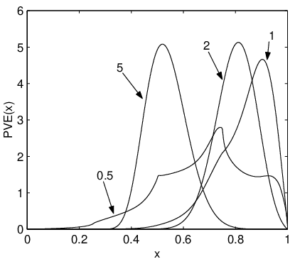
where and is the Heaviside step function. Note that exhibits a divergence as . Eq. (7) is solved by expanding in a suitable set of basis functions on the interval , resulting in an eigenvalue problem. Fig. 1 shows the resulting distributions for four values of . Clearly the statistics of is very non-Gaussian.
The calculations summarised above are not only of interest in the case of one locus, as the following paragraphs show (in the following denotes the number of loci).
Two loci. In the case of two loci () on the same stretch of DNA, the joint distribution of allelic frequencies depends on the rate of gene exchange. Consider (for large )
| (9) |
In the limit of large , the two genealogies for and are essentially independent and the frequencies are well approximated by (3) for each (and large ). The distribution is thus obtained from the single-locus by convolution. The resulting distribution is shown in Fig. 2. Empirically determined recombination rates are often so large that this result for is a good approximation: in Fig. 2 two distributions of are shown, for , and and , obtained from Monte-Carlo simulations. One observes good agreement with the prediction (shaded), even for values of as low as . It must be emphasised that the distribution is markedly non-Gaussian. The wiggles in the Monte-Carlo results are statistically significant; they are a consequence of the finite sample size ().
Many loci. When , and in the limit of large , the distribution of [as defined in (9)] is Gaussian, and its moments are obtained as
| (10) |
Discussion. In an empirical data set, (and ) are necessarily finite. It must then be asked: to which extent are the independently and identically distributed for finite (and )? Fig. 3(a) shows -values determined from empirical data on C. jejuni [21], at the locus GltA ( and ), in comparison with the theory for . The empirical are approximately identically distributed, except at the edges where finite-size effects are observed (remember that ). Monte-Carlo simulations for and confirm the effect of finite sample size. Fig. 3(b) is a similar plot with data taken from one Monte-Carlo sample. The inset of Fig. 3(b) shows that that the are indeed independently distributed. It can be concluded that the theory works well in the present case.
In the remainder two implications of our results are discussed. First, in practice it is necessary to decide whether empirically observed frequencies at a given locus are consistent with the neutral process. The standard statistical test (see [2] p. 263) uses the distribution of as an input (albeit with the number of allelic types as a parameter and not as in the above equations). Since the distribution of was unknown, it was usually determined by Monte-Carlo simulations. Now, however, the result (7,8) can be used: for , eqs. (7,8) apply independently of whether or is taken as the parameter. The corresponding distributions are compared to Monte-Carlo data [20] in Fig. 1. Shown are two cases: and . In both cases, the agreement between our results and those of Monte-Carlo simulations is very good.
Second, many recent empirical studies (see for instance [13, 14, 22]) have analysed the extent of gene exchange. A common measure is the variance of the number of pairwise differences at all loci under consideration. In the limit of (linkage equilibrium) (for the neutral process this evaluates to to , see [12]). However for finite values of (linkage disequilibrium), and especially for small , the expected value of is larger. The empirically determined value of can be compared to a critical value obtained under the null hypothesis that all loci are in linkage equilibrium. The corresponding null distribution is usually obtained using Monte-Carlo simulations [13, 14].
In cases where the neutral model applies, the null distribution of can be determined from eqs. (5), (7) and (8). Consider first the case of large , where the null distribution is approximately Gaussian. Using for large , one obtains
| (11) | |||||
This variance is always larger than the corresponding quantity in a random shuffling scheme [13, 14] because the latter is conditioned on the homozygosity, and not on . When is small, the null distribution will be very non-Gaussian, as the above results for the distribution of show. In Fig. 4, the null distribution of [as determined from (7,8)] is shown for the case of and for four values of . Note that the forms of the distributions imply large, asymmetric confidence intervals. Finally, for , the distributions in Fig. 4 are insensitive to whether the process is conditioned on fixed or fixed [23].
Conclusions. We have shown that distribution functions of empirical observables measuring genetic diversity in selectively neutral populations may exhibit strong non-Gaussian tails. We have found analytical approximations for these distributions, valid for large sample sizes and in the limit where gene exchange is frequent; and have discussed implications for the statistical analysis of genetic variation. It is highly desirable to extend the present results to the case where gene exchange is rare, corresponding to clonal or nearly clonal populations.
References
- [1] M. Kimura and J. F. Crow, Genetics 49, 725 (1964).
- [2] W. J. Ewens, Mathematical population genetics (Springer, Berlin, 1979).
- [3] R. R. Hudson, in Gene genealogies and the coalescent process, Vol. 7 of Oxford Surveys in Evolutionary Biology (1990), pp. 1–44.
- [4] W. J. Ewens and G. Grant, Bioinformatics (Springer, Berlin, 2001).
- [5] http://www.mlst.net .
- [6] International Human Genome Sequencing Consortium, Nature 409, 860(2001).
- [7] J. C. Venter et al., Science 291, 1304 (2001).
- [8] J. Maynard Smith, J. Evol. Biol. 7, 525 (1994); Th. Wiehe, J. Mountain, P. Parham, and M. Slatkin, Gen. Res., Camb. 75, 61 (2000); M. Bahlo, Theor. Pop. Biol. 56, 265 (1999); C. Wiuf and J. Hein, Genetics 155, 451 (2000).
- [9] T. Ohta, Bioessays 18, 673 (1996); M. Kreitman, Bioessays 18, 678 (1996); N. Takahata, Curr. Op. in Gen. & Dev. 6, 676 (1996).
- [10] J. F. C. Kingman, Stochastic Processes and their applications 13, 245 (1982).
- [11] S. Tavaré, in: Calculating the secrets of life: applications of the mathematical sciences to molecular biology (NAP, Washington, D. C., 1995).
- [12] R. R. Hudson, J. Evol. Biol. 7, 535 (1994).
- [13] V. Souza et al., Proc. Natl. Acad. Sci. USA 89, 8389 (1992).
- [14] B. Haubold and P. B. Rainey, Molecular Ecology 5, 747 (1996).
- [15] A. H. D. Brown, M. W. Feldman, and E. Nevo, Genetics 96, 523 (1980).
- [16] Ewen’s sampling formula [2] determines the probability of any neutral sample configuration, as well as the probabilities of these samples conditional on the number of allelic types. Numerical simulations based on this formula are described in: P. A. Fuerst, R. Chakraborty, and M. Nei, Genetics 36, 455 (1977).
- [17] R. Arratia and S. Tavaré, Adv. Math. 104, 90 (1994).
- [18] G. P. Patil and C. Taillie, Bull. Internat. Stat. Inst. 47, 497 (1977).
- [19] P. Donnelly, Theor. Popul. Biol. 30, 271 (1986).
- [20] G. A. Watterson, Genetics 88, 405 (1977).
- [21] K. E. Dingle et al., J. Clin. Microbiology 39, 14 (2001).
- [22] M. C. J. Maiden et al., Proc. Natl. Aca. Sci USA 95, 3140 (1998).
- [23] Note, however, that for small any error in its estimation may influence the distribution of , see Fig. 4.