Spatial diffusion in a periodic optical lattice: revisiting the Sisyphus effect
Abstract
We numerically study the spatial diffusion of an atomic cloud experiencing Sisyphus cooling in a three-dimensional linlin optical lattice in a broad range of lattice parameters. In particular, we investigate the dependence on the size of the lattice sites which changes with the angle between the laser beams. We show that the steady-state temperature is largely independent of the lattice angle, but that the spatial diffusion changes significantly. It is shown that the numerical results fulfil the Einstein relations of Brownian motion in the jumping regime as well as in the oscillating regime. We finally derive an effective Brownian motion model from first principles which gives good agreement with the simulations.
pacs
PACS. 32.80.Pj Optical cooling of atoms, trapping - 42.50.Vk Mechanical effects of light on atoms, molecules, electrons and ionsI Introduction
Laser cooling and trapping was one of the major advances of the last part of the 20th century. In 1997, the Nobel prize in physics was awarded to Steven Chu, Claude Cohen-Tannoudji and William D. Phillips for their works in this domain [1], in particular, for their discovery of the Sisyphus cooling effect [2] which permits to achieve sub-Doppler temperatures and is widely used in various different laser cooling schemes [3]. The Sisyphus effect in optical lattices [4] was studied in a large variety of systems and of field configurations. A large number of results were obtained on temperature, localization and spatial order [5] and an excellent agreement between the experimental observations and the theoretical predictions was found. Much less work has been done to study the spatial diffusion in optical lattices, but also for this problem a reasonable agreement was found between the models [6, 7, 8] and the experiments [6, 9, 10, 11]. However, no detailed study of the dependence of spatial diffusion on, for example, the different directions of an anisotropic lattice or on the size and shape of lattice sites has been performed so far. Very recently, optical lattices and atomic transport therein has attracted new attention with the study of quantum chaos [12] and the achievement of Bose-Einstein condensation by purely optical means [13].
Spatial diffusion in one-dimensional (1D) Sisyphus cooling schemes is fairly well understood. In the so-called jumping regime, where an atom undergoes several optical pumping cycles while moving over one optical wavelength, the atomic motion can be understood by a simple model of Brownian motion [2, 14]. In this regime, spatially averaged friction coefficients and momentum diffusion coefficients have been derived and the validity of the Einstein relations
| (1) |
and
| (2) |
where is the steady-state temperature, the Boltzmann constant, and the spatial diffusion coefficient, has been shown. On the contrary, in the so-called oscillating regime, where an atom travels over several optical wavelengths before being optically pumped into another internal state, the friction force has been shown to be velocity-dependent [2, 14],
| (3) |
where denotes the capture velocity of Sisyphus cooling. In this situation, an analytical derivation of the spatial diffusion coefficient has still be found [6], but an interpretation in terms of a simple Brownian motion no longer works. In particular, it is found in Ref. [6] that the behavior of the spatial diffusion coefficient as a function of the atom-light interaction parameters (laser light intensity and detuning) is dramatically different in the oscillating regime compared to the jumping regime.
In higher dimensional setups, such a difference of the spatial diffusion behaviors in the jumping and the oscillating regimes is expected, too. Moreover, the important difference of the mean free path of a diffusing atom in these regimes may induce different behaviors of the spatial diffusion coefficients as a function of the lattice periods. These are the main issues considered in the present paper.
In this work we perform a detailed study of spatial diffusion in the so-called 3D-linlin lattice [15]. Using semiclassical Monte-Carlo simulations we find that equalities of the form of Eqs. (1) and (2) still hold in the oscillating regime. This suggests that an interpretation by a Brownian motion should still be possible. We derive such a model from basic principles assuming a thermal spatial distribution and taking into account some specific properties of our optical lattice and find a good quantitative agreement with the numerical results. In particular, we calculate an effective friction coefficient in a range of parameters containing both the jumping and the oscillating regimes. We find that in the oscillating regime, increases with the lattice beam intensity and decreases when increases, in strong opposition to the friction coefficient calculated in the jumping regime.
Our work is organized as follows. In Sec. II we describe the specific laser and atom configuration for the 3D optical lattice that we consider here and discuss several important features of the optical potential surfaces. In Sec. III, we present a physical picture of spatial diffusion in periodic optical lattices and we particularly forecast a dramatic change of the behavior of the spatial diffusion coefficients not only versus the atom-light interaction parameters but also versus the geometrical parameters (spatial lattice periods) when going from the jumping to the oscillating regime. In Sec. IV we derive an effective Brownian motion model which we compare in the following sections with the numerical results on the steady-state temperature (Sec. V) and on the spatial diffusion (Sec. VI). Numerical results on the friction coefficient are then discussed in Sec. VII and the validity of the Einstein relations is shown. Finally, we summarize our results in Sec. VIII.
II Sisyphus cooling in the 3D-linlin configuration
The Sisyphus effect cools a cloud of multi-level atoms when a laser field induces spatially modulated optical potentials and pumping rates in such a way that a moving atom on average climbs up potential hills before it is optically pumped into a lower lying potential surface [2]. In this case kinetic energy is converted into potential energy which is subsequently carried away by a spontaneously emitted photon, thereby reducing the total atomic energy.
In this paper we study the so-called 3D-linlin configuration [15]. It is obtained from the standard 1D-linlin configuration [2] by symmetrically splitting each of the two laser beams into two parts at an angle and , respectively, with the () axis in the () and () planes respectively. The resulting configuration consists of two pairs of laser beams in the () plane and in the () plane, respectively, as depicted in Fig. 1, with orthogonal linear polarizations. An important property of this configuration in contrast to 3D setups built of more than four laser beams is that the interference pattern and thus the topography of the lattice does not change because of fluctuations of the relative phase between the various laser beams. Instead, such fluctuations only induce displacements of the lattice.
As in most theoretical work, we will consider atoms with a ground state of angular momentum 1/2 and an excited state of angular momentum 3/2. Experiments usually fall into the low saturation regime defined by
| (4) |
where is the saturation parameter for an atomic transition with a Clebsch-Gordan coefficient of one, is the Rabi frequency for one laser beam, the detuning of the laser beams from the atomic resonance frequency, and the natural width of the atomic excited state. This domain is known to lead to the lowest temperatures. In this situation we may adiabatically eliminate the Zeeman sublevels of the excited state, leading to a theory which only involves the ground state sublevels of angular momentum [14].

An atom in state then experiences an optical potential given by
| (5) | |||||
where
| (6) |
is the light shift per beam and
| (7a) | |||||
| (7b) | |||||
| (7c) | |||||
with the laser wavenumber. The optical potentials are then periodic in the three directions of space with periods . Equation (5) shows that has the same functional dependence on and on but a different one on . We will therefore in the remainder of the paper concentrate on a two-dimensional subsystem only depending on and while fixing . Previous comparisons between 1D and 2D models have shown that the general behavior of the dynamic variables is the same in different dimensions but that scaling factors appear [6]. We thus expect that the results of our work give physical interpretations to full 3D laser cooling schemes but exact numerical values will be changed. Moreover, we will assume a single lattice angle since this gives rise to a vanishing mean radiation pressure force in all directions. The general shape of the optical potential is plotted in Fig. 2.

In the 3D-linlin configuration, the bottom of each potential well is harmonic in first approximation with main axis , and and with the following frequencies:
| (8a) | |||
| (8b) | |||
| where denotes the recoil frequency. | |||
The optical pumping time is
| (9) |
where is the optical pumping rate. The jumping regime corresponds to a domain where , that is, when an atom undergoes many optical pumping cycles during a single oscillation or during a flight over a single potential well. On the contrary, the oscillating regime corresponds to . In this case, an atom can oscillate or travel over many wells without undergoing any pumping cycle. Note that in a 3D-linlin optical lattice, the regimes can be different in different directions because of the geometrical dependence of the border between the jumping and the oscillating regimes,
| (10) |
The asymmetry between the and directions can be seen most easily in a plot of the optical potentials along the and axis, respectively, as shown in Fig. 3. These have different shapes and particularly the crossing between both potential curves is higher in the transverse direction () than it is in the longitudinal one (). As we will see later, this induces significant differences in the cooling and diffusion properties.

As the starting point for the theory presented here we use the standard Fokker-Planck equation (FPE) of the semiclassical laser cooling theory [8, 17, 18] where the external degrees of freedom of the atoms are treated as classical variables. This is obtained from the Wigner transform [19] of the full quantum master equation for external as well as internal degrees of freedom under the assumption of a momentum distribution which is much broader than a single photon momentum, . The FPE for the populations of reads
| (11) |
Here and summation over and is assumed. In this equation, is the jumping rate from the Zeeman sublevel to the sublevel , represents the radiation pressure force and the momentum diffusion matrix for atoms in the internal state . and are the corresponding quantities associated with jumps between different internal states [16]. Note that all these coefficients only depend on the atomic spatial position [17, 18].
A numerical solution of the FPE can be obtained by averaging over many realizations of the corresponding Lan-gevin equations [20]. Such a realization consists in following the trajectory of a single atom which jumps between the two optical potential surfaces corresponding to the two internal states with the appropriate probabilities. Between subsequent jumps the atom experiences potential and radiation pressure forces as well as random momentum kicks which mimic the momentum diffusion according to the coefficients of the FPE. We have performed a large number of such semiclassical Monte-Carlo simulations in order to investigate the dependence of the steady-state temperature, the friction coefficient, and in particular the spatial diffusion coefficient on the various lattice parameters such as detuning , light shift , and lattice angle . We will discuss these numerical results later in Secs. V, VI, and VII.
III Physical picture of spatial diffusion
As a result of the Sisyphus effect, the atoms are cooled and trapped in the potential wells and optical lattices are usually described as atoms well confined in regularly arranged sites (note that in the linlin lattice, the spatial periods of these sites are , the trapping sites corresponding alternatively to and potential wells). However, in bright optical lattices the atom confinement is not perfect because of the strong interaction with the laser light. Two different processes then produce atomic displacements between different trapping sites, inducing spatial diffusion (see Fig. 4). For the sake of simplicity, we describe these processes in one dimension but they occur analogously in higher dimensional setups.
On the one hand (see Fig. 4 left), a trapped atom still undergoes fluorescence cycles and thus takes random recoils due to photon absorption and re-emission. Hence, the oscillating motion of the atom gets perturbed. Particularly, the atom can explore regions where its potential energy ( if the atomic internal state is ) is not minimum (). In such regions, optical pumping cycles preferentially transfer the atom into the lower potential curve and the atom is cooled and trapped in the neighboring potential well (elementary Sisyphus cooling process). This process induces atomic transfers from a site to a neighboring one in another potential curve.
On the other hand (see Fig 4 right), when a trapped atom oscillates in a potential well, it has a small but non zero probability of being optically pumped into the upper potential curve. In the jumping regime the atom is immediately pumped back into its initial trapping potential well. This effect thus induces heating and noisy oscillating trajectory of the atom leading indirectly to spatial diffusion via transfers between neighbouring potential wells. On the contrary, in the oscillating regime the atom is not immediately re-pumped and travels over several potential wells before undergoing an elementary Sisyphus cooling process again which traps it into another potential well.
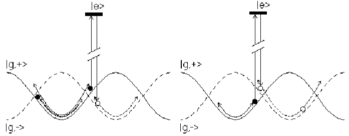
The diffusion process linked to optical pumping is much more efficient than the one due to recoils except for very small laser detunings [14]. We will thus focus on the second process to describe spatial diffusion in periodic multi-dimensional optical lattices. We will see that the differences of this process in the jumping and the oscillating regimes induce a dramatic difference in the behavior of the spatial diffusion coefficients.
In a simple model, we can describe the diffusive behavior of the atomic cloud as random walks of atoms between periodic trapping sites [21]. Let us assume that an atom is trapped in one specific potential well and jumps after a time to another well. The spatial diffusion coefficient in the direction is
| (12) |
where is the mean free path in direction .
In the jumping regime, as discussed above, an atom essentially transfers from a trapping site to a neighboring one and thus . The life time of an oscillatory external state is on average of the order of [22], independently of . Hence, and
| (13) |
In the oscillating regime, an atom travels over several lattice sites before it is trapped again. Here where is the average velocity with the atomic mass and the time of one flight. As it will be justified in Secs. IV and V, is proportional to independently of and . is of the order of again[22]. Hence,
| (14) |
Note that we implicitly assume straight line flights and we do not consider anisotropic effects. Obviously, because of the potential shape and anisotropy, a dependence of on , and should be added in Eq. (14) but our simple model does not provide its determination. Nevertheless, in the case of a strong anisotropy (), the setup is almost one-dimensional in the i-direction so it is expected that does not depend on . Indeed, at large space scale, the length of one flight of a particle moving on a 1D-periodic potential is independent of the periodicity.
We want to emphasize that these discussions are only valid for lattice parameters far away from the domain of décrochage for spatial diffusion. For small potential depths, rare long flights dominate the diffusion which therefore becomes anomalous [7].
IV Brownian motion model
Before turning to a detailed discussion of the numerical results, we will now derive a simple analytical model which will help to understand the main features of the cooling scheme.
The basic idea of this model is to consider the atomic dynamics as a Brownian motion, as it has been successfully applied to Doppler cooling [14] and 1D Sisyphus cooling in the jumping regime [2, 14], but taking some properties of localization into account [23, 24]. The fundamental ingredients are therefore the derivation of an average friction force and an average momentum diffusion coefficient.
Let us consider an atom at position moving with a constant velocity . In this case the FPE (11) reduces to
| (15) | |||||
where we used . The jump rates are
| (16) |
Expanding the populations in powers of the velocity in the form and inserting into Eq. (15), yields the stationary solutions
| (17a) | |||||
| (17b) | |||||
with the operator
| (18) |
Formally, the velocity and position dependent level populations can thus be written as
| (19) |
The total force averaged over the internal atomic states is then given by
| (20) |
In order to derive a space and velocity averaged friction force in the form we now have to make certain assumptions on the stationary atomic distribution.
In 1D laser cooling one usually assumes a flat spatial distribution of the atoms in the lattice. However, as we have seen in Sec. II, the shape of the 3D optical potential differs significantly in the different directions. In particular the potential barrier between neighboring potential wells is much higher in the transverse than in the longitudinal direction. From Eq. (5) and Fig. 3 we see that in the direction the potential depth is of the order of whereas we will see later that the steady-state temperature is of the order of . Therefore we expect strong localization in that direction. On the contrary, in the direction the potential depth is of the order of and the atoms will be less localized. Instead of a flat spatial distribution of the atoms we will thus assume a thermal distribution
| (21) |
corresponding to the optical potential averaged over the internal atomic state and for a given, yet unknown, temperature . Let us emphasize that assuming a thermal distribution is not a priori justified for laser cooled samples but show significant quantitative deviations from such a simple behavior [25, 26]. In fact, our numerical simulations give actual spatial distributions in qualitative agreement with Eq. 21 but show significant quantitative deviations from such a simple behavior. However, we only use this approximation here to obtain a qualitative understanding of the exact results obtained numerically and we will see later that our results derived here are in good quantitative agreement with the simulations.
Because of the symmetry of , only terms containing odd powers of the velocity in contribute to the averaged force. We may thus restrict ourselves to
| (22) |
As a further simplification we will now also average over velocity and therefore replace by
| (23) |
where is the spatial average with respect to . Equation (23) is obtained by substituting , , () in Eq. (18). From this we finally get the friction coefficients
| (24) |
with
| (25a) | |||||
| (25b) | |||||
Along the lines of [27] and using the same approximations as for the friction, we derive averaged momentum diffusion coefficients
| (26) |
with
| (27a) | |||||
| (27b) | |||||
For simplicity we have not written a term of the momentum diffusion which arises from the random recoil of absorbed and spontaneously emitted photons. This varies as and thus can be neglected for large detuning ().
In a model of Brownian motion, the steady-state temperature then fulfills
| (28) |
that is, averaging Eq. (1) over the and directions. The right hand side is obtained from Eqs. (24) and (26) which themselves depend on the temperature via Eq. (21). Thus, Eq. (28) yields an implicit equation for which can be solved numerically, e.g., by iteration of Eqs. (21)-(28) recursively. Note that no lattice parameter, such as the lattice angle or the laser detuning, appears in this equation. is thus strictly proportional to and independent of and . We find
| (29) |
This temperature can then be used to determine the following numerical values:
| (30) |
and
| (31) |
Finally, we want to derive an approximate expression for the spatial diffusion coefficients. To this end, we must again take the atomic localization into account. While Eq. (1) for the relation between temperature, momentum diffusion coefficient and friction coefficient approximately holds for trapped and untrapped atoms, the corresponding equation (2) for the spatial diffusion only holds for free atoms. Indeed a cloud of completely trapped atoms achieves a stationary spatial distribution and hence shows no spatial diffusion. Using Eq. (29) and the assumption of a thermal momentum and spatial distribution, we calculate numerically that a fraction of 55.6% of all atoms have a total energy above the potential depth along , and a fraction of 15.3% above the potential depth along as discussed before. Taking only these free atoms into account, we finally obtain effective spatial diffusion coefficients, which correspond to those observed in the numerical simulations or in actual experiments, in the form
| (32) | |||||
This expression is in good qualitative agreement with our physical discussion (see Sec. III) in both the jumping and the oscillating regime. We will further discuss this point in Sec. VI.
V Steady-state kinetic temperature
We performed a systematic study of the temperature and the spatial diffusion as a function of the lattice parameters, exploring a large domain containing both the jumping and the oscillating regime. More precisely, we performed numerical semi-classical Monte-Carlo simulations with the following parameters:
In this and the following sections we present the results of the simulations and compare them with the analytical model discussed above. All of our discussions and conclusions rely on the complete set of data, even if the figures only contain a few sample curves for the sake of clarity.
We first study the atomic cloud steady-state temperature resulting from the competition between slowing and heating processes. We calculate the average square velocity over the whole atomic cloud at each time step of the simulations. The temperature in direction is then given by
| (33) |
A second method to obtain the temperature numerically is to fit a Gaussian to the simulated momentum distribution. We have checked that the widths of these Gaussians indeed give the same temperatures as those obtained from Eq. (33). For a broad initial velocity distribution, the temperature first decreases in time (thermalization phase), but finally reaches a steady state.
The thermalization time lies between and for large enough lattice angles ( in the simulations), but for it is approximately in the transverse direction. In this case, the spatial period is large and an atom needs to fly a long time to undergo efficient Sisyphus cooling. Such an increase of the cooling time is also observed in the longitudinal direction for large angles but is less important because does not reach very large values.

Both the transverse and the longitudinal temperatures are shown in Fig. 5 versus the laser detuning for a fixed lattice angle and for several light shifts per beam. This exhibits two domains where the temperature behaves differently. For small detunings () we find a rapid decrease of the temperature with increasing , whereas for large detunings the temperature is independent of but increases approximately linearly with . This agrees well with the general form
| (34) |
where , and () are numerical factors, as, for example, has been found in Ref. [18]. The first term of Eq. (34) has not been found in Sec. IV because in the momentum diffusion, Eq. (26), we neglected the term due to absorption and spontaneous emission.
Let us first concentrate on the oscillating regime, . In Fig. 6 we plot the temperature versus the lattice spatial period for various laser detunings and light shifts in this domain. We find that the temperature is nearly independent of the lattice angle, i.e., of the spatial periods. The temperature is thus strictly linear in the potential depth and independent of any other lattice parameter as predicted by Eq. (29). Such a property has been observed experimentally [28] but we emphasize that our result here holds for a broader range of parameters in the oscillating regime as well as in the jumping regime. A linear fit to the numerical results gives
| (35a) | |||||
| (35b) | |||||

In the range of parameters investigated here, these values of the temperatures agree with Eq. (29) with an accuracy of about .
Equations (35) show that the temperature is anisotropic, , which is in good agreement with experimental observations by A. Kastberg and coworkers [29]. This is a consequence of the asymmetry between the transverse and longitudinal directions for the optical potential in the linlin lattice. In the physical picture of Sisyphus cooling [2, 14], cooling ends once an atom is trapped in a single potential well and hence the steady-state temperature is proportional to the potential depth. As already discussed in Sec. IV this is about twice as large in the transverse direction as in the longitudinal. Hence, the transverse temperature would be expected to be about twice as large as the longitudinal. However, correlations between these two directions tend to equilibrate the temperatures and in the simulations we therefore find to be only about times larger than .
We now turn to the jumping regime, . We find a completely different behavior of the temperature. This is a consequence of the increasing contribution of absorption and spontaneous emission to the force fluctuations [28]. Physically, an atom experiences many photon recoils during one elementary cooling process and is thus more likely to escape from the trapping potential. Hence, the atom can reach a steady state temperature larger than the potential well depth.

VI Spatial diffusion of the atomic cloud
We now turn to the study of the spatial diffusion of the atomic cloud. In the simulations we calculate the average square position in each direction over the whole cloud.
In the thermalization phase the hot atoms follow almost ballistic trajectories and the cloud expands rapidly. For longer times the expansion reaches a normal diffusion regime where
| (36) |
and is a constant depending on the initial space and velocity distribution. Note that does not depend on this initial distribution as we verified in the simulations.

In Fig. 8 we plot the transverse and longitudinal spatial diffusion coefficients versus the lattice detuning for various light shifts and for a given lattice angle. Figure 8 clearly shows two domains where the spatial diffusion coefficient behaves differently. For small detunings, decreases rapidly with and increases with , whereas for large detunings, increases with and does not depend on except for . The latter corresponds to a relatively shallow potential and the system is close to the transition to anomalous diffusion [6, 7, 28].
Fitting the numerical results with an expression of the form of Eq. (32), we find:
| (37) |
The coefficients of this fit are in good quantitative agreement with the analytical result (32). The main difference is the factor of 1.39 which amounts to the difference between the longitudinal and the transverse temperatures as found in Sec. V. Figure 8 shows that Eq. (37) yields an excellent fit to the numerical data. From Eq. (10) and Eqs. (32), (37) we observe that the two domains where behaves differently correspond to the jumping and the oscillating regimes.
In the jumping regime we find:
| (38a) | |||||
| (38b) | |||||
in good qualitative agreement with our physical discussion in Sec. III, see Eq. (13). In particular, is proportional to as shown in Fig. 9 and proportional to the optical pumping rate . The different values of the numerical coefficients indicate that the trapping is stronger in the transverse direction than in the longitudinal, in agreement with our discussion in Sec. IV.

On the contrary, in the oscillating regime we find:
| (39a) | |||||
| (39b) | |||||
In this regime, is proportional to as expected from Eq. (14) and the angular dependence is qualitatively given by Eq. (32). In Fig. 10 we show this angular dependence in the oscillating regime. Here, the transverse and longitudinal directions are not independent because the potential wells significantly deflect the trajectories of atoms travelling over many optical potential wells. The dependence of on thus contains both and . This is dramatically different to the situation in the jumping regime where atoms only jump between adjacent wells. Equation (39) also confirms that for , does not depend on as predicted in Sec. III.

VII Friction force
The theoretical model of Sec. IV was based on the description of the atomic dynamics by a Brownian motion model. Let us now further investigate the validity of such a description by testing in the numerical simulations some characteristics of Brownian motion. We particularly perform a direct numerical measurement of the friction coefficients and test the validity of the Einstein relation (2).
In order to probe the atomic dynamics we submit the atoms to a constant, space and velocity independent force in addition to the forces due to the atom-light interaction. In an experiment this could be provided simply by gravity or, for example, by the radiation pressure force of an additional weak laser beam. In a Brownian motion model such a constant force will give rise to a constant mean velocity of the atomic cloud with
| (40) |
Because of the linearity of the Brownian equations of motion the kinetic temperature and the spatial diffusion coefficients are not changed.
Adding such a constant force in the numerical simulations along the -direction, we observed in fact that the atomic cloud experiences a drift in this direction at a constant velocity. In the ideal case of a pure Brownian motion any amplitude of can be used, but in the case of Sisyphus cooling the friction coefficient is velocity dependent. In order to get proportional to , it is thus essential to use a small enough force which induces a global drift much smaller than the width of the velocity distribution. Under this condition the temperature and the spatial diffusion do not depend on and Eq. (40) can be used to numerically find unique friction coefficients .

We can then compare these numerical results with the friction coefficient obtained via the Einstein relation (2) using the numerically found values of the temperature (see Sec. V) and of the spatial diffusion coefficient (Sec. VI). In Fig. 11 we plot the ratio of these two friction coefficients and find deviations of about 15%. Hence, the dynamics of an atomic cloud in an optical lattice is in reasonable agreement with a two-dimensional Brownian motion model. Note that the eigen-directions of the motion are the and directions in good agreement with the theoretical model.
In order to better understand this result let us briefly return to the model developed in Sec. IV. As has been shown in the previous section, the numerically obtained diffusion coefficient agrees well with the analytical result (32). In the derivation of the latter we have assumed that the cloud of atoms can be split into a trapped fraction and into a free fraction. Only the free atoms were taken into account for the spatial diffusion. Similar arguments must also be considered for the friction coefficient. Adding a small constant force will leave a trapped particle in its initial potential well, and therefore the fraction of trapped atoms does not contribute to the mean velocity of the cloud. Thus, the measured friction coefficient using Eq. (40) should be given by the analytical result (24) divided by the fraction of free atoms. Hence, for the measured values of the spatial diffusion and of the friction both sides of Eq. (2) are corrected by the same factor. In other words, the Einstein relation holds because the measured quantities only involve the freely travelling atoms for which a Brownian motion model works well.
Therefore, we obtain an analytic fit to the measured friction coefficient by inserting Eqs. (35) and (37) into Eq. (2). We find
| (41a) | |||||
| (41b) | |||||
These approximate expressions are compared with the numerically obtained values of the friction coefficient in Fig. 12. We see that there is excellent agreement both qualitatively and quantitatively.
The behavior of is again different in the jumping and the oscillating regime. In the jumping regime, is proportional to and approximately independent of [2, 14]:
| (42a) | |||||
| (42b) | |||||
However, Fig. 12 exhibit a small dependence of versus in the jumping regime and this is not forecasted by the model. In fact, the kinetic temperature is not proportional but linear in and this induce a dependence of the spatial distribution in . Coefficients are thus -dependent and this can explain the discrepancy.
In the oscillating regime, is proportional to and depends on both and as discussed in Sec. VI:
| (43a) | |||||
| (43b) | |||||
The expression found in the simulations is in good qualitative agreement with the expression derived in the theoretical model Eq. (43). Note however that coefficients are not given by Eq. 30 but are to be calculated considering the free atoms which contribute to spatial diffusion only.

VIII Conclusions
In conclusion, we performed a systematic study of the behavior of an atomic cloud in a linlin optical lattice with the help of semi-classical Monte-Carlo simulations. We explored a broad range of lattice parameters including the jumping and the oscillating regime.
The temperature was found to be linear in the potential depth and independent of the laser detuning and of the lattice angle in a broad range of parameters. We have shown that the temperature is anisotropic, the transverse one being larger than the longitudinal one by a factor of . All these results are well explained with the help of the physical picture of Sisyphus cooling and are in good agreement with experimental results.
The spatial difusion was studied in the regime of normal diffusion. The behavior of differs significally in the jumping and in the oscillation regimes. In the first, decreases with and increases with . In the second, increases linearly with and does not depend on . The behavior of as a function of the lattice spatial periods is also different in both regimes: whereas is proportional to in the jumping regime, it is a function of as well as in the oscillating regime. This reveals correlations between the transverse and longitudinal directions of the lattice.
By adding a constant force in the Monte-Carlo simulations we could numerically measure the friction coefficients and we showed that the Einstein relations are fulfilled. This supports a description of the dynamics in terms of Brownian motion. The friction coefficient is proportional to and in the jumping regime. In the oscillating regime, is proportional to and , and the dependence on the lattice geometry involves both and .
The numerical results have been found to be in good agreement with a simple theoretical model based on a semi-classical approach. We derive the steady-state temperature, the friction force, and the spatial diffusion from a model of Brownian motion taking into account atomic localization in the optical potential wells. To explain the measured friction and spatial diffusion, the atomic cloud must be split into a trapped part and a free part. While in general both parts contribute to the internal and external dynamics, only the free fraction of atoms is responsible for the observed expansion of the cloud and for the drift of the center of mass under the influence of a weak constant force.
The spatial diffusion of atomic clouds in optical lattices is usually studied in pump-probe spectroscopy experiments, using the properties of the Rayleigh line [30]. However, the validity of this method has never been proven. We expect that the models discussed here will serve to this verification by providing a systematic theoretical study of the directly measured spatial diffusion coefficients.
Finally, it should be noted that our restriction to has been guided by experimental restrictions but is not necessary. Indeed, when this condition is not fulfilled, the unbalanced radiation pressure induces a fast escape of the atomic cloud from the optical lattice which makes experimental investigations difficult. Nevertheless, this situation could be of great interest because it offers the opportunity of studying optical lattices with different spatial periods along the and axes and interesting anisotropic effects could be found.
Acknowledgements.
We are indebted to Yvan Castin for numerous enlightening discussions. We also thank Anders Kastberg’s group for the communication of their experimental results before publication. Laboratoire Kastler-Brossel is an unité de recherche de l’Ecole Normale Supérieure et de l’Université Pierre et Marie Curie associée au Centre National de la Recherche Scientifique (CNRS). This work was partially supported by the European Commission (TMR network “Quantum Structures”, contract FMRX-CT96-0077) and the Austrian Science Foundation FWF (project P13435-TPH and SFB “Control and Measurement of Coherent Quantum Systems”).References
- [1] S. Chu, Nobel Lectures, Rev. Mod. Phys. 70, 685 (1998); C. Cohen-Tannoudji, Nobel Lectures, ibid 70, 707 (1998); W. D. Phillips, Nobel Lectures, ibid 70, 721 (1998).
- [2] J. Dalibard and C. Cohen-Tannoudji, J. Opt. Soc. Am. B 6, 2023 (1989); P. J. Ungar, D. S. Weiss, E. Riis and S. Chu, ibid B 6, 2058 (1989).
- [3] for a review of laser cooling, see H. J. Metcalf and P. van der Straten, Laser cooling and trapping, Springer-Verlag, Berlin (1999).
- [4] J. S. Jessen and I. H. Deutsch, Adv. At. Mol. Opt. Phys. 37, 95 (1996), and references therein.
- [5] G. Grynberg and C. Mennerat-Robilliard, Phys. Rep., 355, 335 (2001).
- [6] T. W. Hodapp, C. Gerz, C. Furtlehner, C. I. Westbrook, W. D. Philipps and J. Dalibard, Appl. Phys. B 60, 135 (1995).
- [7] M. Holland, S. Marksteiner, P. Marte, and P. Zoller, Phys. Rev. Lett. 76, 3683 (1996); W. Greenwood, P. Pax and P. Meystre, Phys. Rev. A 56, 2109 (1997).
- [8] S. Marksteiner, K. Ellinger, and P. Zoller, Phys. Rev. A 53, 3409 (1996).
- [9] C. Jurczak, B. Desruelle, K. Sengstock, J. Y. Courtois, C. I. Westbrook and A. Aspect, Phys. Rev. Lett. 77, 1727 (1997).
- [10] H. Katori, S. Schlipf and H. Walther, Phys. Rev. Lett. 79, 2221 (1997).
- [11] A. G. Truscott, D. Baleva, N. R. Heckenberg, H. Rubinsztein-Dunlop, Opt. Commun. 145, 81 (1998).
- [12] Special issue “Quantum transport of atoms in optical lattices”, J. Opt. B: Quantum Semiclass. Opt. 2, 589-703 (2000), edited by M. Raizen and W. Schleich.
- [13] M. D. Barrett, J. A. Sauer, and M. S. Chapman, Phys. Rev. Lett. 87, 010404 (2001).
- [14] C. Cohen-Tannoudji, Les Houches summer school of theoretical physics 1990, Session LIII, in ”Fundamental systems in Quantum Optics”, J. Dalibard, J. M. Raimond and J. Zinn-Justin editors, North Holland, Amsterdam, Elsevier Science Publishers B.V., (1991).
- [15] K. I. Petsas, A. B. Coates and G. Grynberg, Phys. Rev. A 50, 5173 (1994); A. Kastberg, W. D. Phillips, S. L. Rolston, R. J. C. Spreeuw, and P. S. Jessen, Phys. Rev. Lett. 74, 1542 (1995).
- [16] K. I. Petsas, G. Grynberg and J.Y. Courtois, Eur. Phys. J. D 6, 29 (1999).
- [17] Y. Castin, K. Berg-Sørensen, J. Dalibard, and K. Mølmer, Phys. Rev. A 50, 5092 (1994).
- [18] P. Horak, J. Y. Courtois and G. Grynberg, Phys. Rev. A 58, 3953 (1998).
- [19] E. P. Wigner, Phys. Rev. 40, 749 (1932).
- [20] H. Risken, The Fokker-Planck equation, Springer, Berlin (1989).
- [21] C. Itzykson and J. M. Drouffe, Statistical Field Theory vol. 1: From Brownian Motion to Renormalization and Lattice Gauge Theory, Cambridge University Press, Cambridge (1991).
- [22] J. Y. Courtois and G. Grynberg, Phys. Rev. A 46, 7060 (1992).
- [23] A. Görlitz, M. Weidemüller, T. W. Hänsch, and A. Hemmerich, Phys. Rev. Lett. 78, 2096, (1997); M. Weidemüller, A. Görlitz, T. W. Hänsch, and A. Hemmerich, Phys. Rev. A 58, 4647 (1998).
- [24] M. Gatzke, G. Birkl, P. S. Jessen, A. Kastberg, S. L. Rolston, and W. D. Phillips, Phys. Rev. A 55, R3987 (1997).
- [25] C. Gerz, T. W. Hodapp, P. Jessen, K. M. Jones, W. D. Philipps, C. I. Westbrook and K. Mølmer, Europhys. Lett. 21, 661 (1993).
- [26] K. Mølmer and C. I. Westbrook, Laser Physics 4, 872 (1994).
- [27] J. Dalibard and C. Cohen-Tannoudji, J. Opt. Soc. Am. B 2, 1707 (1985).
- [28] F. R. Carminati, M. Schiavoni, L. Sanchez-Palencia, F. Renzoni and G. Grynberg, Eur. Phys. J. D, in press (2001).
- [29] A. Kastberg et al., private communication.
- [30] J. Y. Courtois, and G. Grynberg, Adv. At. Mol. Opt. Phys. 36, 87 (1996).