Analysis of dynamical and measurement noise Chaos- low dimensional Langevin method Markov processes Noise-statistical physics
On a quantitative method to analyze dynamical and measurement noise
Abstract
This letter reports on a new method of analysing experimentally gained time series with respect to different types of noise involved, namely, we show that it is possible to differentiate between dynamical and measurement noise. This method does not depend on previous knowledge of model equations. For the complicated case of a chaotic dynamics spoiled at the same time by dynamical and measurement noise, we even show how to extract from data the magnitude of both types of noise. As a further result, we present a new criterion to verify the correct embedding for chaotic dynamics with dynamical noise.
pacs
05.45.-apacs
05.10.Gpacs
02.50.Gapacs
05.40.C1 Introduction
Handling noise in experiments is a challenging task for an experimenter during everyday work regardless of the field he or she is working on. Any knowledge of the nature of the involved noise is important to understand experimental results. It may help to estimate the achievable precision to make out noise induced effects or to set up models for the experimental system under investigation. For a general application it is essential that these methods should require as little knowledge as possible of the system.
In this paper we present evidence that it is possible for measured data, which were spoiled by different types of noise, to separate two basic types of noise and to measure their magnitudes. To show the quality of our method we apply it to the case of a noisy nonlinear chaotic dynamical system. Obviously, this method also works for simpler dynamical situations, which are frequently given in experimental research.
Before the early 80s complex, disordered systems were explained predominantly by stochastic models. The complex behavior of the dynamic was described by random motions. Then it became clear that many of these disordered systems might be generated by low dimensional nonlinear deterministic dynamics. For both kinds of systems a lot of refined methods for data analysis were developed, cf. [1, 2, 3, 4, 5, 6, 7, 8]. Complications in the data analysis based on this clear distinction arise if noise is present beside a nonlinear deterministic dynamics. Two basic types of noise can be distinguished, namely, dynamical noise, which acts directly on the dynamics, and measurement noise, which is only added to the signal of the dynamics. Thus, for the analysis of disordered systems it is one fundamental problem to characterize the type of noise and to quantify the amount of noise.
Recently, a method was proposed whereby dynamical noise and measurement noise can be measured very precisely, if the dynamical equations are known [9]. Our paper is devoted to the problem of unknown dynamics. It is our intention to show that it is possible by pure data analysis to clarify which kind of noise is present. Furthermore, by using the theory of diffusion processes one is able to estimate the magnitude of dynamical and measurement noise. Our proceeding is based on recent works [3, 12, 13, 14] showing that it is possible to reconstruct from given data the underlying stochastic processes and we want to point out that it is not founded on any previous knowledge given by models of the dynamic or by some assumed parameterizations.
The structure of the paper is as follows: First we describe the mathematics we are using for the reconstruction of the deterministic flow in phase space from given data sets. Next it follows the criterion for the distinction between measurement noise and dynamical noise. We demonstrate that this method can be successfully applied to measured data of the chaotic Shinriki oscillator, which are perturbed by different types of noise. At last we show that the signal of the dynamical noise and its correlation can be extracted from the measured data. This can be taken to examine the nature of the stochastic process and to verify the sufficient high embedding of a chaotic noisy system.
2 Concepts of stochastic processes
Based on the mathematics of diffusion processes it has recently been realized that by directly using the definition of the Kramers-Moyal coefficients [10, 11] it is possible to reconstruct the dynamics of the Langevin equation from given data [3, 12, 13, 14]. This idea is the foundation of the following presentation.
First we focus on the wide class of nonlinear dynamical systems with dynamical noise, also known as the diffusion processes. It can be represented by a Langevin equation (in the Itô representation),
| (1) |
where denotes the time dependent -dimensional stochastic state vector. The drift coefficients, , represent the deterministic part of the dynamics, and the diffusion coefficients, , determine the strength of the dynamical noise, including the general case of multiplicative noise when the coefficients depend on . is -correlated Gaussian noise (Langevin force).
As known from [10], the drift coefficients are obtained as the limit of conditional moments
| (2) | |||||
| (3) |
and the diffusion coefficients by the moments
| (4) | |||||
| (5) |
The numerical estimations of these conditional moments are performed for , for a sufficiently small neighborhood of a fixed value in the phase space. These conditional moments can be estimated directly from given data sets in a parameter free way. For small (i.e. smaller than the recurrent time [15]) the first two moments () are connected to the diffusion coefficient [17, 18]:
| (6) |
If, in addition to the dynamical noise, also measurement noise is present the procedure of the estimation of has to be changed. The measurement noise, which is typically added by the process of measuring data, can be formulated mathematically as
| (7) |
The vector is the sum of the state vector described by the dynamics of Eq. (1) and measurement noise. Here the measurement noise is given by its standard deviation and the -correlated noise term . As a consequence of the definition (7), it is easy to see that for the conditional moments, as defined in Eqs. (3) and (5), one obtains
| (8) | |||||
Note that for the determination of via (see equation (3)) no correction term appears due to the measurement noise, because it averages out.
The equation (8) is valid for a sufficient small neighborhood so that and can be approximated by constant values in . Furthermore the linear dependence of on can be taken as a criterion for a correct sampling frequency, which has to be chosen so high that this linearity is resolved.
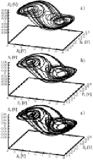
Next we apply the method to measured data of a chaotic electronic oscillator. As a circuitry we have chosen the Shinriki oscillator [21] as shown in Fig. 1. In Fig. 2 exemplary phase space representations of the attractors for the measured data are shown. Fig. 2a) shows the pure deterministic chaotic dynamics, Fig. 2b) the dynamics with dynamical noise, and Fig. 2c) dynamics with the combination of dynamical and measurement noise. For an experimental realisation of the dynamical noise, a -correlated noise source is in series connection to the negativ resistor. The corresponding Langevin equation for the three voltages , describing the Shinriki oscillator, see Fig. 1, are given by
| (9) | |||||
| (10) | |||||
| (11) |
where describes the Langevin force. For the specific parameters see Fig. 1, the negative resistor and describes the nonlinearity of the Zener diodes. An empirical formular for the characteristic curve is
| (12) |
where . The four parameters , , and have to be fitted on the measured characteristic curve. Additional measurement noise was added to the data, namely to the component .
[width=3in]figure1.eps
To give evidence of the validity of our procedure for the case of dynamical noise, we show in Fig. 3 the reconstructed deterministic part of Eq. (9), which we obtained from measured data (here and in the following we use 400.000 data points for our analysis). Here an exemplary cut through has been chosen in such a way that the nonlinearity becomes obvious. By measuring the electronic elements ( and ) we can directly compare the characteristics gained from Eq. (9) with the reconstructed one (see Fig. 3). The small deviations can be explained by parasitic capacitances and inductances. For analogous numerically generated data sets no significant deviation of the reconstructed values of was found.

Furthermore, we investigate the diffusion coefficients. For simplification, only the case of additive noise is considered, i.e. is constant. According to equations (3), (5) and (8) we calculate . To improve the statistics we calculate the median of about the whole state space. As shown in Fig. 4 the moments display a linear dependence on small [22]. The slope of this dependence gives the strength of the dynamical noise , see Eq. (8). Most remarkably shows an increasing off-set when the measurement noise is increased. According to equation (8) with the value of the strength of the measurement noise can be measured. Our results are summarized in table 1. The precision of these results obviously depends on the number of data points. Furthermore we notice that with increasing magnitude of the measurement noise the value gets underestimated while the precision of the estimated almost remains about constant. ( corresponds to about noise.)

| [V] adjusted | 0.0 | 0.12 | 0.24 |
|---|---|---|---|
| [V] estimated | -0.011 | 0.11 | 0.20 |
| [V/] adjusted | 7.9 | 7.9 | 7.9 |
| [V/] estimated | 8.4 | 8.5 | 8.4 |
An important consequence of this method should be noted. In the case of pure dynamical noise it is easy to see from Eq. (1) that the knowledge of and makes it possible to extract from measured data the noise term . Based on this, it can be quantified whether the noise is -correlated or not. As an illustration the autocorrelation of the reconstructed noise is shown in Fig. 5a). Note that correlations are expected if the inserted noise is not -correlated. To investigate such a case we use a too low dimensional phase space embedding of our measured data. In Fig. 5b) the autocorrelation of the reconstructed noise is shown for the case that the data of Fig 5a) are reduced to a two-dimensional projection of the dynamics on and . In this case the unresolved variable together with represent correlated noise. This result clearly shows two points: (a) the validity of a Markov process (i.e. the noise is -correlated) can be verified; (b) if correlations are found, like those shown in figure 5b), the system does not obey a Markov process.

To conclude, in this paper we show for the first time, that based on the well known theory of diffusion processes, and especially based on the estimation of the Kramers-Moyal coefficients it is possible to analyze the kind of noise given in time series. The method shown here does not depend on previous knowledge of the underlying nonlinear deterministic dynamics. This does not imply that our method must work for any dynamical process. From an experimental point of view, the obtained results have to be verified whether the correct dynamics is grasped by the reconstructed process. Therefore the acting noise can be extracted and the typical dynamics can be obtained by numerical integration of the reconstructed phase flow using the obtained values of . If this is successful, a further improvement of the estimation of the reconstructed process can be achieved by parameterizing the results of our method and successively applying procedures for parameter estimation like [9, 16].
Acknowledgements.
Helpful discussions with S. Siegert, Ch. Renner, H. Kantz as well as the hospitality of the Max-Planck Institute for the Physics of Complex Systems, Dresden are acknowledged.References
- [1] \NameSchreiber T. Kantz H. \BookNonlinear time series analysis \PublCambridge university press \Year1997
- [2] \NameHilborn R. C. Tufillaro N. B. \REVIEWAm. J. Phys.651997822.
- [3] \NameSiegert S., Friedrich R. J. Peinke \REVIEWPhys. Lett. A2431998275-280.
- [4] \NameBorland L. Haken H. \REVIEWZ. Phys. B81199295.
- [5] \NameBorland L. Haken H \REVIEWAnn. Physik11992452.
- [6] \NameKlimontovich Y. L. \REVIEWInt. Journ. of Bif. and Chaos31993119.
- [7] \NameStark M. R. J., Broomhead D. S., Davies M. E. Huke J. \REVIEWNonlinear Analysis-Theory Methods & Applications3019975303.
- [8] \NameMuldoon M. R., Broomhead D. S., Huke J. P. Hegger R. \REVIEWDynamics and Stability of Systems131998175.
- [9] \NameHeald J. P. M. Stark J. \REVIEWPhys. Rev. Lett.8420002366.
- [10] \NameKolmogorov A. N. \REVIEWMath. Ann.1401931415-458.
- [11] \NameMoyal J. E. \REVIEWJ. Roy. Stat. Soc.111949195-197.
- [12] \NameRenner Ch., Peinke J. Friedrich R. \REVIEWJ. of Fluid Mech. 4332001383-409.
- [13] \NameFriedrich R., Siegert S., Peinke J., Lück St., Siefert M., Lindemann M., Raethjen J., Deuschl G., Pfister G. \REVIEWPhys. Lett. A 2712000217-222.
- [14] \NameGradisek J., Siegert S., Friedrich R., Grabec I. \REVIEWPhys. Rev. E6220003146-3155.
- [15] Here we used 77.5 samples per mean recurrent time, corresponding to a sampling rate of 66 kHz. Problems arising for large are discussed in [16].
- [16] \NameTimmer J. \REVIEWChaos, Solitons and Fractals1120002571.
- [17] \NameRisken H. \BookThe Fokker-Planck equation \PublSpringer-Verlag Berlin \Year1984
- [18] An expansion of to higher order terms in is given in [19, 20].
- [19] \NameRagwitz M. Kantz H. \REVIEWPhys. Rev. Lett.872001254501.
- [20] \NameFriedrich R., Renner Ch., Siefert M. Peinke J. arXiv:physics/0203005.
- [21] \NameShinriki M., Yamamoto M. Mori S. \REVIEWProc. IEEE691981394.
- [22] Investigations without this averaging leads to similar results.