[
Geometric and Statistical Properties of the Mean-Field HP Model, the LS Model and Real Protein Sequences
Abstract
Lattice models, for their coarse-grained nature, are best suited for the study of the “designability problem”, the phenomenon in which most of the about 16,000 proteins of known structure have their native conformations concentrated in a relatively small number of about 500 topological classes of conformations. Here it is shown that on a lattice the most highly designable simulated protein structures are those that have the largest number of surface-core switchbacks. A combination of physical, mathematical and biological reasons that causes the phenomenon is given. By comparing the most foldable model peptides with protein sequences in the Protein Data Bank, it is shown that whereas different models may yield similar designabilities, predicted foldable peptides will simulate natural proteins only when the model incorporates the correct physics and biology, in this case if the main folding force arises from the differing hydrophobicity of the residues, but does not originate, say, from the steric hindrance effect caused by the differing sizes of the residues.
pacs
PACS number: 87.10.+e, 87.15.-v, 87.15.By]
I Introduction
It is believed that the dynamical folding of a protein to its native conformation is determined by the amino acid sequence of the protein [1]. Yet the folding of any particular protein is an extremely complex process; simulation of the folding of even a small protein remains an unsurmounted challenge to state-of-the-art computers [2]. Nevertheless, a good understanding of a number of general features of protein folding have been acquired in computational studies using simple lattice models [3, 4, 5, 6, 7, 8]. One feature is the so-called funnel picture that leads to a two-state description of folding [5, 9]. Here the vertical dimension of the funnel represents the state of foldedness of the protein (or roughly its free energy), which increases (decreases) from the top towards the bottom of the funnel, and a cross-section of the funnel represents the conformation space accessible to the folding protein at a given state of foldedness. Near the top of the funnel, most conformations are freely accessible and folding proceeds extremely rapidly. As the folding progresses and the opening of the funnel narrows, accessibility of one conformation from another becomes increasing restrictive, so that increasingly fewer pairs of conformations are connected by almost-equal-energy paths and folding correspondingly slows down. An alternative view is that the energy landscape becomes increasingly rugged. At some junction the rate of decrease in the number of accessible conformations, hence the rate of decrease in entropy, is so large as to cause the rate of free-energy change as a function of foldedness to be positive, so that a free-energy barrier is formed to become an obstacle against further folding. At this point folding practically grinds to halt and can proceed stochastically only on very rare occasions that brings it over the barrier, after which the protein folds (and unfolds) relatively rapidly to its native conformation in an annealing-like process.
Another issue clarified by simple lattice models is the designability of ”topological” classes of protein conformations [6, 7, 10]. The designability of a conformation class is the number of proteins whose native conformations belong to the class. At the moment the number of proteins with known three-dimensional conformations in the Protein Databank (PDB [11]) is of the order of 16,000 and is increasing rapidly, while the number of conformation classes has remained about 500 for some time and is not expected to grow beyond 1000. Even when the the fact that many proteins in the PDB are homologues with similar structures are taken into account, the discrepancy between the number of non-homologous proteins and the number of conformation classes of observed native conformations is glaring. Because a class is in fact composed of many conformations that differ in detail (such differences could very well be important to the function of proteins), the problem of designability is best studied in coarse-grain models, such as lattice models, that disregard such details.
The simplest interacting lattice model is the HP model proposed by Dill et al. [3], in which the 20 kinds of amino acids are divided into two types, hydrophobic (H) and polar (P). This model has been studied extensively by several groups in the last decade [3, 4, 5, 6, 7, 8]. A mean-field version of the model that yields tremendous simplification was used to study the designability problem, and it was found that the designabilities of structures vary greatly (the terms structures and conformation classes will be used interchangeably in this paper), and that only a tiny portion of structures are highly designable. Moreover, it was noted that highly designable structures seem to have patterns that emulates secondary structural motifs [6, 7, 10].
In a general Hamiltonian setting, the Hamiltonian can be viewed as a mapping of the peptide space to the conformation space . When is sufficiently coarse grained, which is the case we consider, each point in is a topological class of native conformations. Then is a mapping of to such conformation classes into . If we remove from all the peptides that are mapped by to more than one conformation class in (i.e., the degenerate cases), the remainder of is partitioned by into equivalent classes of peptides, with each peptide class being mapped to a single conformation class. Designability results from a highly skewed distribution of the size of the peptide classes. We shall call peptides belonging to peptide classes that are mapped to highly designable structures highly foldable peptides.
In [7] the designability issue of the mean-field HP model was reduced to a purely geometric problem which rendered it easy to discuss and visualize the skewed distribution of the size of peptide classes. It was however not made clear what characterizes those structures that are highly designable, nor was it demonstrated whether or not highly foldable peptides have anything to do with real proteins. In fact, whereas one can well imagine many ’s in lattice models to yield biased designability, it is not clear that any such would yield foldable peptides that simulate real proteins.
In this paper, expanding on claims made in an earlier letter [10], the highly designable structures in the mean-field HP model will be characterized - they are those that have the largest number of surface-core switchbacks, and it will be shown that highly foldable peptides have a high similarity with real protein sequences in general and with segments of sequences that fold to helices in particular.
To demonstrate a point made above, this paper also discusses a lattice model that exhibits designability but does not seem to be biologically correct. In the LS model, the 20 kinds of amino acids are divided into two types, large (L) and small (S), and it is assumed that the deciding factor in folding is the the steric hindrance effect caused by the difference in the sizes of the amino acids [12]. It was shown in ref. [12] that on a lattice, structures in the LS model too have uneven designability (there called encodability score); only a small portion of structures, also claimed to have protein-like secondary structures, are selected by large numbers of peptide sequences as unique ground states. It will be shown here that in spite of the fact that the LS model is mathematically almost equivalent to the mean-field HP model, unlike the mean-field HP model, highly foldable peptides in the LS model do not match well with real protein sequences.
In the following two sections the mean-field HP model and the LS model are reviewed and it is shown that, notwithstanding their quite different physical contents, on square lattices the two models are mathematically close approximates. In Section 4 the geometrical properties of a two-dimensional square lattice and the way they restrict the space of structures, which are compact paths on the lattices, are discussed. In Section 5 it is shown that only a very small portion of the structure have the highest numbers of surface-core switchbacks and that, for both models, it is these structures that have the highest designabilities. Because the partition of amino acids in the HP model is based on hydrophobicity while that in the LS model is based on residue size, the highly foldable peptides are translated into different sets of “physical” peptides in the two models. In Section 6 the highly foldable peptides in the two models are compared with real proteins in the Protein Data Bank and it is shown that the highly foldable peptides in the HP model match well with real protein sequences in general and with segments of sequences that fold to helices in particular (but not well with segments of sequences that fold to sheets), whereas those in the LS model match poorly with real protein sequences. Section 7 gives an expanded discussion of our results. In an Appendix the most highly foldable peptides in the two models are given and compared.
II The HP Model
The Hamiltonian of the HP model is:
| (1) |
where is the type, H for hydrophobic and P for polar, of the th residue, or amino acid, in the peptide chain [3]; if and are nearest neighbors in the lattice but not adjacent along the peptide sequence, and otherwise; specifies the residue contact energies that depend on the types of residues in contact.
Several sets of contact energies have been used: for the original HP model [3], by Li et al. [6], and by Buchler and Goldstein [13]. Li et al. suggested that the contact energies should satisfy the following constraints: 1) compact shapes have lower energies than non-compact shapes; 2) so that hydrophobic residues are buried as much as possible; and 3) different types of residues tend to segregate, which is a condition induced by having [6, 14]. In this work these will be adopted with the modification that 3) is replaced by the additive relation . Then the potential simplifies to:
| (2) |
where for H and for P residue [15]. Henceforth only structures that correspond to self-avoiding compact paths on a lattice will be considered.
In an two-dimensional square lattices, there are four corner sites with coordination number , side sites with and core sites with . With the exception of the two ends of the peptide chain, which we ignore, each lattice point has contacts. So the Hamiltonian Eq.(1) becomes:
| (3) | |||||
The first term on the right-hand side of Eq.(3) is a constant for a given peptide sequence. It is independent of whatever conformation the peptide resides in and, since Eq.(3) will only be used here to determine the native structure of a particular peptide sequence, it will be omitted. The third term means that it is costly to put H residues in the corner sites. Since it is of order it too will be omitted. The Hamiltonian then simplifies to what is known as the mean-field HP model [7]:
| (4) |
where , , is the binary peptide sequence and is a binary structural sequence converted from a self-avoiding compact path on the lattice with the assignment: (0) if the th site of the structure is a core (surface) site. In this new form the Hamiltonian has an interpretation quite different from its original meaning. There it was an expression of inter-residual interaction. Here in Eq. (4) it is no longer inter-residual, rather it has the form of a site-dependent potential. With fixed for a given lattice and a constant for a given peptide sequence, both are irrelevant to the determination of the ground state structure of the peptide. They will be ignored in the ensuing calculation. The Hamiltonian now reduces to one-half of and a neat geometric interpretation for it emerges [7]. When and are viewed as -component vectors, this quantity is just the Hamming distance between two corner points in a unit -dimensional hypercube.
III The LS Model
It was shown by Micheletti et al. that in the LS model the designability (called encodability score by the authors) distribution of structures is similar to that in the mean-field HP model [12]. The Hamiltonian of this model is
| (5) |
where ; is the maximal number of nearest contacts without steric repulsion belonging to residue ; on a square lattice, is equal to 1 (2) for () residues inside the chain, and to 2 (3) for () residues at chain ends; is the number of contacts of the th residue in a conformation ; and equals to 1 if and otherwise. The Hamiltonian implies that if the number of contacts of the th residue is larger than , then the contact energy will be increased by owing to steric effects.
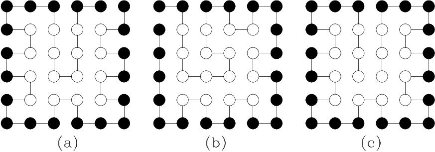
The results in Ref. [12], where was set equal to , show that the distribution of designability of structures in LS model is very similar to that in the HP model. In fact most of the highly designable structures in one model are likewise in the other model (see Appendix). The highly designable structures in the LS model also have protein-like secondary substructure and tertiary symmetries. Three among the most designable structures in the two models are shown in Fig. 1.
Just as practiced in the last section, we consider only compact structures and neglect the effect of the two end points on a peptide chain. Table 1 gives the values of , and Hamiltonian for the two types of residues at corner, side and core sites on a square lattice. Let , and denote the number of corner, side and core sites, respectively; = + + = the total number of sites; and the subscripts and denote residue type, then
| (6) | |||||
For a given peptide sequence, and are fixed. First consider the case when the steric repulsion is strong but finite, namely, . Dropping the corner term one gets for a given peptide sequence,
| (7) |
where p and s are the peptide and structure binary vectors defined before, with the exception that in p the digit 0 (1) now stands for L (S). Comparison of this equation with Eq. (4) reveals that, at least on a square lattice, the mathematical form of the two models are essentially identical, provided that here the pair H and P in the HP model is replaced by S and L, respectively. Since there is only one scale in either model, the size of does not matter so far as it is much greater than unity but finite.
| type | corner | side | core | |
| 0 | 1 | 2 | ||
| 2 | 1 | 0 | ||
| S | 1 | 1 | 1 | |
| 0 | -1 | -2 | ||
| 1 | 0 | -1 | ||
| L | 1 | 1 | -a | |
| 0 | -1 | 2a |
IV Geometrical Properties of the 2D Square Lattice
Since Eqs. (4), (7) and (8) reduce the Hamiltonians of the mean-field HP and LS models to the same problem in geometry, namely one of the Hamming distance between the two vectors s and p, we now study the space of these vectors (in the HP model). Consider an square lattice with sites. Recall that every structure is a self-avoiding compact path on the lattice. The set of all binary peptides p is then just the set of binary sequences. Because of geometric constraints, the set of binary structure sequences s is far smaller than . For a very rough estimate for the upper limit of the size of , consider the construction of compact paths by random walk on the lattice. At any given point during the walk after the first step, the maximum number of allowed next steps is the coordination number minus one, which is between 2 and 3. As the number of steps taken increases, the average number of allowed next steps will decrease. We take the average number to be 2 up to the point when the lattice is half full. For a randomly chosen path, after the lattice is half full, chances are that the number of allowed next steps will be either one or zero most of the time. So the number of allowed s’ should be much less than . On a 66 lattice this last number is 262144, whereas the size of is 30408, and the size of is . An example of an allowed s on the 66 lattice is shown in Fig. 2 (a). If we think of as the set of all the corner points in the -dimensional unit hypercube, then the set is composed of a tiny subset of corner points. It was shown earlier that the designability of an s is the Voronoi polytope of s in ; it is clear what characterizes the designability problem is the distribution of the contents of in the unit hypercube.
We now examine how geometric constraints reduce down to . A sequence in may be viewed as a chain of 0’s and 1’s connected by links of three types, those connecting 0 and 0 sites, 0 and 1 or 1 and 0 sites, and 1 and 1 sites, respectively. Let the numbers of such links be , and , respectively. The sequence is partitioned by the 1-0 links into segments of contiguous 1’s or 0’s. Whereas the link numbers for a p are devoid of geometric meaning, that for s are the consequences of geometric constraints. To illustrate this, consider the case (the surface to core ratio in smaller lattices are too lop-sided to be of interest). Some of the simplest constraints that must be satisfied by an allowed s are:
- 1.
An isolated single 0 may only occur at an end of a path;
- 2.
An isolated single 1 may only either occur at or be one 0-segment away from an end of a path;
- 3.
Each of the four corners on the lattice belongs to a 0-segment at least 4 sites long, except when the corner is an end of a path;
- 4.
For a path having the pattern s (both the ends of the path are 1-sites), and ;
- 5.
For s , and ;
- 6.
For s , and if , the last relation is replaced by if ;
- 7.
For s , and ;
- 8.
For s and , and ;
- 9.
For s , and .
The first two rules are obvious on a square lattice. The third rule implies that the polar residues tend to accumulate around corners. This fortuitously reflects a property of real proteins: the relative abundance of polar residues on surface areas with large curvatures. Figs. 2 (b) and (c) illustrate the origin of the fourth rule on a 66 lattice. The two structures are both of the type , that is, they begin and end both on core sites. The dark solid links in the figures define “templates” for constructing s’ that respectively have the maximum (twelve) and minimum (two) values for . Rules (5)-(8) can be shown in a similar way. By explicitly applying the above rules in the selection of s (as opposed to requiring an s to be a compact self-avoiding path), the total number of binary sequences in is reduced to a set of candidate paths which, relatively speaking, is now only slightly greater than the exact number () of s’ in . This implies that the set of rules given above embodies the essence of the geometric requirement that guarantees elements in to be compact self-avoiding paths.

V Distribution of the Allowed Structures in the Hypercube
Here we show that only a small portion of the structures in have large . On an square lattice, there is a total of links and among them need to be chosen to form a structure. For the 66 case these numbers are 60 and 35, respectively. For the structure shown in Fig. 2 (b), of the total number of 60 links on the lattice, 28 links are used to define the template (that has =12) and 17 links, marked by filled diamonds in the figure, are forbidden because they would form close loops or connect sites which already have two links. This means that to complete an s from the template, one needs to select links from among links on the lattice. Hence at most s’ with = 12 can be constructed from the template. A similar argument shows that s’ with = 2 can be constructed from the template shown in Fig. 2 (c), which has 21 predetermined links. The ratio 817190 : 6435 illustrates the point that the number of s’ with high values is much smaller than the number of s’ with low values.
We now give a heuristic argument showing that there is an approximate relation between the smallest possible Hamming distance between two structures and and the difference in the values of the two structures, =; for simplicity we assume that . For this discussion we ignore the two end points of the structures, so that (on a square lattice) all the segments on an s partitioned by 0-1 links have at least two 0 or two 1 digits. We begin by considering the case when =. Then both and are zero. Suppose we can generate by swapping the positions of a pair of 0’s and a pair of 1’s in (while keeping in mind that in most cases such an operation would not give an s; it would give a p that is not in ). Then = 2 and, depending on the position of the replaced pair of 0’s in , = 0 or 2. Any other pair of and having = 2 will have 2. Thus is 2 for = 2. Similarly, if we generate by exchanging the positions of a pair of 0’s and a pair 1’s in , for example:
| (9) |
| (10) |
then = 4 and = 2 (Eq.(9)) or 4 (Eq.(10)). Again any other and having = 2 or 4 will have 4. Thus is 4 for = 4. Arguing along this line it can be shown that .

In Fig. 3, the logarithmic distributions of the Hamming distances between pairs of s’ with fixed values of are plotted for a 66 lattice. The relation between and is clearly displayed. Notice that all distributions peak at a Hamming distance of 15-20, with the width of the distribution decreasing monotonically with .


It has already been shown that the number of s’ with large is much smaller than the number of s’ with small . Hence the former kinds of s’ will be even more sparsely distributed in than the latter kinds. Thus given an arbitrary s the chances are that most of its nearest neighbors will have relatively small ’s. An s with large will be farther away from its nearest neighbors than if it has a smaller . This is indeed brought out in Fig. 4, where each curve plots as a function of the number of neighboring s’ in within a Hamming distance , averaged over those s’ specified by . It is seen that so long as , s’ with large has far fewer nearby neighbors (in ) than s’ with smaller . It follows that s’ with large will on average have large Voronoi polytopes, hence high designabilities. Note that the approximate proportional relation between and is not expected to be limited to square lattices although the proportional constant is expected to be dependent on lattice type.
| lattice | ||
|---|---|---|
| 6 | 4 | |
| 9 | 8 | |
| 10 | 7 | |
| 11 | 10 | |
| 12 | 9 | |
| 66 | 14 | 12 |
| 21-site triangle | 12 | 9 |
In Fig. 5 (a) and (b) the logarithmic designability is plotted as a function of for a 66 square lattice and a 21-site triangular lattice, respectively. The size of each disc indicates the number of s’ having the specific and designability and an open diamond indicates the average designability of all s’ having the specified . On the whole the average designability increases with up to near the maximum . For near the maximum value it appears that the heuristic argument given above breaks down, probably partly for boundary effects, and partly because the number of structures with the largest values of is very small (3 for and 24 for among the 30408 s on a 66 square lattice) so that statistical fluctuations become important. The designability distributions on several other lattices were studied and the pattern shown in Fig. 5 persisted. The result is summarized in Table 2, where , the maximum and , the where the largest average designability occurs, are given for each lattice. In all the cases . Results for three-dimensional lattices will be shown elsewhere.
VI Comparison with Real Proteins
It has been shown that the mathematical contents of the mean-field HP model and the LS model are essentially identical. The physical (or biological) interpretations given to the two models are however entirely different. The mean-field HP model is based on the assumption that hydrophobic residues would congregate in the core as much as possible. The LS model is based on the assumption that large residues would be excluded from the core as much as possible. To see which model is closer to Nature we compare the results of the two models with real proteins by matching model peptide sequences against protein sequences culled from data banks. For either model, the model sequences are the two sets of sequences among a total randomly sampled 36-word binary sequences that select the most highly designable and least designable structures, respectively, on a 66 lattice.
We consider the frequency distributions of the set of sequences {}, where the subscript denotes the concatenated 27006 peptides mapped to the 15 most highly designable structures in the mean-field HP model; , the concatenated 24134 peptide sequences mapped to the 1545 least designable structures in the mean-field HP model; S, the concatenated 22789 peptides mapped to the 364 most highly encodable structures in the LS model [16]; , the concatenated protein sequences in PDB [11], converted to a binary sequences based on the hydrophobicity of the peptides; , same as , but includes only segments of protein sequences that fold to helices; , same as , but includes only segments of protein sequences that fold to sheets; , and , same as , and , respectively, except that protein sequences are converted to binary ones based on the volume of residues. The ten residues designated polar (P) are: Lys, Arg, His, Glu, Asp, Gln, Asn, Ser, Thr, Cys [17] and the ten residues designated as L-type residues are, in descending order of volume, Trp, Tyr, Phe, Arg, Lys, Leu, Ile, Met, His and Gln [18]. That the HP and LS models differ in physical and biological contents is predicated by the fact that the two lists overlap poorly. This predication will not change if the cut-off points of either or both lists are varied slightly. The sequences h and S will be referred to as the most foldable peptides in the HP and LS models, respectively.
To compare the sequences, we employ a Cartesian coordinate representation for symbolic sequences [19], here applied to binary sequences. Let denote the set of binary strings of length . Given a binary sequence of length and a string length (we are interested only in cases when ), there is the set of frequencies of occurrence of the string in . The frequencies may be obtained, say, by counting while sliding a window digits wide along . The frequency depends on the ratio of 0 to 1 digits in the sequence. This ratio, , is 0.983, 1.039, 0.553, 0.960, 0.993, 0.720, 0.734, 0.917 and 0.934, respectively, for the sequences , = . In order to make a fair comparison of the sequences adjustments need to be made to compensate for the disparity in the 0 to 1 ratios. For this purpose we define a normalized frequency by
| (11) |
where is the number of 0’s in . Sequences in the normalized frequency set now have 0 to 1 ratios equal to unity.
In what follows we consider only cases when is even, . Let be a lattice with spacing , and be a one-to-one mapping from to , by:
| (12) |
where is a string in and is a site on . From the set we define a normalized relative frequency distribution of on the lattice :
| (13) |
where is the mean frequency and
| (14) |
Figs. 6 and 7 show the distributions , = , , and , and = , , , and , respectively. In the figures, the magnitude of the distribution is coded into the gray scale shown at the top of the figures. From the fact that (b) and (d) in Fig. 6 have their brightest and darkest regions, respectively, at generally the same locations, it is evident that h ((d)), the most foldable peptides in the HP-model, is closest to α ((b)), the sequence that represents helix segments in real protein sequences. In comparison, although (a) looks similar to (b), it is not so similar to (d). In particular, some of the brightest regions in (a) are dark in (d), and vice versa. In sharp contrast (c), which represents sheet segments in real protein sequences, is entirely different from all the other distributions in Fig. 6.
Turning to Fig. 7, it is noticed that (d), representing the most foldable peptides in the LS model, is very similar to its counterpart in the HP model, Fig. 6 (d). This is as expected because the mathematical contents of the two models are essentially identical. On the other hand, (d) is very dissimilar to (a), which represents all protein sequences in PDB, but with the residues partitioned according to the LS model. This shows that size of the residue is not the most dominant factor in protein structure.
The frequency distributions shown in Figs. 6 and 7 are repeated in Figs. 8 and 9, except that the word length is now eight instead of six. This implies that the sequences are now examined with a finer resolution. The result is similar to the case: the most foldable peptides in the HP model closely resemble the helix segments of real protein, while the foldable peptides in the LS model do not resemble real proteins.


The sequences may be compared in a more quantitative manner through the overlap of frequency distributions:
| (15) |
The overlaps , for a number of pairs () selected from the set {}, and for are given in Fig. 10.
One first notices that, with the exception of ( in Fig. 10), all the overlaps approach zero as the word length increases. This is so because the resolving power of the method increases with ; for sufficiently large , the resolution becomes so large that any two sequence that does not have substantial and extended sequence identity will have zero overlap. That has large positive correlation throughout the whole range of studied is expected from the mathematical equivalence of the HP and LS models. In Ref. [12], the parameter in Eq.(5) was taken to be infinity to emphasize the steric constraint on the residues. Here we had done the same just to conform to Ref. [12]. On the other hand, since in the present study all the structures are self-avoiding paths on a discrete lattice, the steric constraint caused by the existence of the backbone is automatically satisfied. Therefore, so far as the intention of the LS model is concerned, a small and positive, but not infinite, value for would have sufficed.


The overlap (filled ) is larger than most other overlaps for much of ’s shown in the figure. This is connected to a basic fact of proteins: helices account for almost half of the total amount of protein sequences in PDB. The overlap drops sharply when 12 because most helix segments are shorter than 15 residues long.
Next in order of magnitude are the overlaps and (filled and ); these have large positive values for the smaller ’s. This reveals that the mean-field HP model provides a coarse-grained description of some features of the real proteins and suggests that the basic assumption of the model - that local residue-water interaction is the dominant cause for protein folding - is consistent with the mechanism for the formation of helices. The overlaps decrease with increasing for the general reason given above. On the other hand, the negative correlation shown by the negative value of the overlap () shows that the same assumption is inconsistent with what causes the formation of sheets. Two of the obvious reasons are: whereas most sheets are buried in the interior of proteins, the mean-field HP model differentiates only surface from core sites but has no means of influencing the interior structure of proteins; the stability of most sheets depends on long-range interactions that are absent in the model.

The negative value of the overlaps between S and (, and , respectively) indicates that the highly foldable peptide sequences in the LS model are anti-correlated with the real protein sequences for and uncorrelated for larger . This confirms what is already seen in Figs. 7 and 9: that size effect is not the dominant factor determining the formation of a stable protein conformation. Finally, the large negative values of the overlap () for all values of tested simply verify that the most and least foldable peptides in the HP model are highly dissimilar however they are compared.
VII Discussion
Because conformation designability in protein structure refers to the natural selection of a very small number of topological classes of native conformations over the vast total number of classes, it is a topic that can be suitably studies in coarse-grained settings such as in lattice models. Previous lattice model studies have firmly established that indeed only a very small number of (model) structures, out of a very large total number, are highly designable. It has not been shown why this phenomenon should arise, and to what classes of native conformations would the highly designable structures correspond. In this paper, taking advantage of the geometric picture for the designability problem given in [7], namely that designability of a structure in the mean-field HP model is proportional to Voronoi volume of that structure in a certain hyperspace, we showed that uneven designability arises because a type of structures - those with the largest numbers of surface-core switchbacks - are very rare, and that their nearest neighbors in the hyperspace are other similar rare structures. Hence such structures have the largest Voronoi volumes and the highest designabilities. Because the hyperspace of structures has properties independent of the two-dimensional lattices used in the present study, this conclusion is expected to stand for other more realistic lattices. Indeed, the same effect was observed on a three-dimensional lattice based on an icosahedron [22].
The identification of structures having the largest numbers of surface-core switchbacks with the conformation classes of observed proteins entails certain physical and biological implications. Proteins choosing such structures as native conformations would tend to have ratios of numbers of H-type and P-type residues close to being unity. Indeed, the averages of H to P ratios for all the protein sequences in PDB, for the segments that folds to helices and and for those that fold to sheets, respectively, are all very close to unity. Proteins having structures with many surface-core switchbacks are expected to be energetically favored. For such proteins would by and large have alternating P and H residues that match the pattern of the structures, and the outward-pointing force exerting on the P-type residues and the inward-pointing force exerting on the H-type residues together would make the protein especially sturdy.
On the mean-field HP lattice, high-designability structures tend not to have long sequences of contiguous sites that are purely core sites or purely surface sites (see Table 3 in Appendix), because such structures tend to be involved in degenerate cases - peptides with corresponding contiguous subsequences of P- or H-type residues (or S- or L-type residues in the LS model) would easily have two or more such structures as ground states - and for that reason the peptide and the degenerate structures would have been excluded from the set of allowed peptides and acceptable structures, respectively. This practice is justified biologically: peptides and conformations involved in degeneracy (in a coarse-grained sense) are presumably filtered out by evolution because they would make for functionally unreliable proteins. In fact, relatively few proteins in PDB have sequences containing long segments of contiguous P- or H-type residues whose native conformations have long segments of contiguous surface or buried sites [23]. Such native conformations are presumably generated by the finer details of inter-residual interactions, and the conformation classes to which they belong would not have counterparts among the high designability structures given by simple, coarse-grained lattice models.
Because structures on square lattices are not realistic enough for direct comparison with empirically observed topological conformation classes, we compared model peptides folding into such structures, namely the most foldable peptides, with (binarized) peptide sequences in the PDB. If the highly designable structures are rich in surface-core switchbacks then the highly foldable peptides should be rich in H and P singlets and HH and PP doublets. In Table 3 in the Appendix it is seen that the the highly foldable peptides in the mean-field HP model are rich in HHPP (or PPHH) but poor in HP (or PH) repeats. This reflects an artifact of the square lattice. On such lattices, the shortest surface-core switchback motif is surface-surface-core-core (or core-core-surface-surface) repeats while surface-core repeats do not exist (see first two “constraints” in Section IV). We showed that the most foldable peptides match well with those segments of protein sequences in PDB that fold into helices but match relatively poorly with segments that fold into sheets. helices are most commonly amphipathic and lie on the outside of their host proteins. With 3.6 residues per turn, such helices tend to change from H to P residues with a periodicity of three to four. That is, they should have a predominance of alternating HH and PP doublets interspersed with H and P singlets. Indeed, of all peptide sequences that code helices in the PDB, 24% of H to P (or P to H) changes are after singlets, 36% are after doublets and 22% are after triplets. This implies that helices are relatively rich in HHPP repeats and this could explain why the most foldable model peptides (in the mean-field HP model) match well with helices.
The situation is different with respect to sheets. The most common domain structures in proteins are / domains that consist of a central group of sheets surrounded by helices. The sheets in these domains will not be rich in either HHPP or HP repeats. In the second large group of protein domain structures, comprised of antiparallel sheets, some of the sheets are on the outside of the protein and these are rich in HP repeats but not in HHPP repeats. A superfamily of proteins containing such sheets has members such as the human plasma retinal-binding protein and -lactoglobulin, a protein that is abundant in milk. Of all peptide sequences that code sheets in the PDB, 33% of H to P (or P to H) changes are after singlets, 28% are after doublets and 18% are after triplets. Hence the most foldable model peptides would match poorly with sheets.
If our computation were carried out on a lattice that allowed structures with surface-core repeats then the foldable model peptides would have better matched sequences coding for sheets. Still, because the only interaction taken into account in the mean-field HP model is the hydrophobicity of the residues, whereas the formation of the majority of sheets depend on other details of interesidual interactions, we cannot expect the most foldable model peptides to have a good match with the majority of sheets irrespective of what lattice was used.
If hydrophobicity but not inter-residual interaction is indeed the main force that drives the formation of helices, then we can better understand why helices are formed on a time scale of the order s [24, 25], right after the collapse of the protein to globular shape, and why it takes ten times longer for the formation of sheets, which involves interactions between residues distantly separated on the primary structure. This scenario is consistent with the finding in a recent statistical analysis of experimental data: local contacts play the key role in fast processes during folding [26].
We have shown that the mathematical content of the LS model, which partitions residues into large (L) and small (S) ones, was essentially the same as that of the mean-field HP model. Hence the binary composition of the most foldable peptides in the two models are quite similar (see Table 3, Appendix). However, because not all large (small) residues are hydrophilic (hydrophobic), the most foldable peptides in the two models are mapped to significantly different sets of (binarized) protein sequences. The result is that the most foldable peptides in the LS model do not match well with any subset of proteins in the PDB. This means that steric hindrance effect arising from different sizes of the residues is not the main driving force for protein folding.
We thank the National Center for High-Performance Computing (NCHC) for providing support in computation and accesses to PDB. This work is partly supported by grants NSC89-2213-E-321-004 to ZYS, NSC89-M-2112-008-0022 to HCL and NSC87-M-2112-007-004 to BLH from the National Science Council. HCL thanks the Physics Department of Stanford University where this work was partly written.
References
- [1] C. Anfinsen, Science 181, 223 (1973).
- [2] Y. Duan and P.A. Kollman, Science 282, 740 (1998).
- [3] K.A. Dill, Biochemistry 24, 1501 (1985); H.S. Chan and K.A. Dill, Macromolecules 22, 4559 (1989).
- [4] E.I. Shakhnovich, Phys. Rev. Lett. 72, 3907 (1994); H.S. Chan and K.A. Dill, Proteins 24, 335 (1996); C. Micheletti, F. Seno, A. Maritan, and J.R. Banavar, Phys. Rev. Lett 80, 2237 (1998); F. Seno, C. Micheletti, A. Maritan, and J.R. Banavar, Phys. Rev. Lett 81, 2172 (1998).
- [5] P.E. Leopold, M. Montal, and J.N. Onuchic, Proc. Natl. Acad. Sci. USA 89, 8721 (1992); P.G. Wolynes, J.N. Onuchic and D. Thirumalai, Science 267, 1619 (1995); J.N. Onuchic, P.G. Wolynes, Z. Luthey-Schulten and N.D. Socci, Proc. Natl. Acad. Sci. USA 92, 3626 (1995).
- [6] H. Li, R. Helling, C. Tang and N.S. Wingreen, Science 273, 666 (1996).
- [7] H. Li, C. Tang, and N.S. Wingreen, Natl. Acad. Sci. USA 95, 4987 (1998).
- [8] E.I. Shakhnovich, Curr. Biol. 8, R478 (1998).
- [9] J.D. Bryngelson and P.G. Wolynes, Proc. Natl. Acad. Sci. USA 84, 7524 (1987); O.M. Becker and M. Karplus, J. Chem. Phys. 106, 1495 (1997); A. Gutin, A. Sali, V. Abkevich, M. Karplus and E.I. Shakhnovich, J. Chem. Phys. 108, 6466 (1998); P. Garstecki, T.X. Hoang and M. Cieplak, Phys. Rev. E60, 3219 (1999).
- [10] C.T. Shih, Z.Y. Su, J.F. Gwan, B.L. Hao, and C.H. Hsieh, and H.C. Lee, Phys. Rev. Lett. 84, 386 (2000).
- [11] Protein Data Bank ver.91, released Jan. 2000; H.M. Berman, J. Westbrook, Z. Feng, G. Gilliland, T.N. Bhat, H. Weissig, I.N. Shindyalov, P.E. Bourne, Nucleic Acids Research, 28, 235-242, 2000.
- [12] C. Micheletti, J.R. Banavar, A. Maritan, and F. Seno, Phys. Rev. Lett. 80, 5683 (1998).
- [13] N.E.G. Buchler, and R.A. Goldstein, Proteins 34, 113 (1999).
- [14] H. Li, C. Tang, and N.S. Wingreen, Phys. Rev. Lett. 79, 765 (1997).
- [15] M.R. Ejtehadi, N. Hamedani, H. Seyed-Allaei, V. Shahrezaei, and M. Yahyanejad, Phys. Rev. E 57, 3298 (1998).
- [16] (It turns out that in the LS model, because an L (i.e., large) residue is strictly forbidden - when - to occupy a core site, for a same set of sample peptides, the encodabilities of highly encodable structures are generally much lower than the designabilities of highly designable structures in HP model.)
- [17] A. Radzicka et al., Biochemistry 27, 1664 (1988).
- [18] A.A. Zamyatin, Prog. Biophys. Mol. Biol. 24, 107 (1972).
- [19] Bai-Lin Hao, and Wei-Mou Zheng, Applied Symbolic Dynamics and Chaos, World Scientific, 1998.
- [20] G.D. Rose, A.R. Geselowitz, G.J. Lesser, R.H. Lee and M.H. Zehfus, Science 229, 834 (1985).
- [21] Wen-Hsiung Li, Molecular Evolution, (Sinauer Associates, 1997) p. 14.
- [22] B.H. Wang and H.C. Lee, unpublished.
- [23] In the peptide obtained from concatenating all the protein sequences in PDB, the average length of contiguous same-type residues is approximately 1.8 residues, with a standard deviation of 1.1 residues. The total number of residues involved in same-type contigs longer than four residues is about 9% of the total number of residues.
- [24] V. Munõz, P.A. Thomson, J. Hofrichter and W.A. Eaton, Nature 390, 196 (1997).
- [25] S. Williams et al., Biochemistry 35, 691 (1996).
- [26] K.W. Plaxco, K.T. Simons and D. Baker, J. Mol. Biol. 277, 985 (1998); H.S. Chan, Nature 392, 761 (1998).
APPENDIX
Here we show how the two lattice models differ by comparing strings of several lengths that have the highest and lowest frequencies of occurrence, called the most and least favored strings, respectively, in the sequences h and S, which are the concatenated sequences of the mostly highly foldable peptides in the mean-field HP and LS models, respectively. In Table 3, the first and sixth columns list such strings. Strings of different lengths are ranked separately by their normalized relative frequency of occurrence (Eq. (14)); the string with the highest (lowest) frequency is ranked 1 (). By definition, an unfavored string has negative frequency. Table 3 shows that the most favored strings are quite well correlated in the two models but the least favored strings are not so. It is seen that among 4-mers the repeats (0011) are the most favored pattern in both models, long repeats of 1’s and 0’s are the least favored string patterns in the HP model favored string patterns in the HP model and (01) is the the least favored string repeat in the LS model. The reason for this is clear: (0011) repeats are the favored pattern in most highly designable structures in both models and each of the (peptide) strings (0000), (1111) and (0101) is separated from (0011) by the greatest frame independent Hamming distance. There is an additional disincentive for a peptide to have (01) repeats in the LS model. On a square lattice such repeats do not appear in a structure sequence, hence, with L-type residues (represented by 0 digits) strictly forbidden on core sites (represented by 1 digits), a peptide string with 01 repeats can only occupy a structure sequence composed entirely of surface sites. This gives the peptide zero binding energy in the LS model. The situation is different in the HP model. There a peptide string with 01 repeats can occupy a structure sequence with 0011 repeats and non-zero binding energy.
| Strings most/least | HP model | LS model | Strings most/least | LS model | HP model | ||||
| favored in HP model | freq. | rank | freq. | rank | favored in LS model | freq. | rank | freq. | rank |
| (0110) | 0.4459 | 1 | -0.0468 | 10 | (0011) | 0.3834 | 1 | 0.4272 | 2 |
| (0011) | 0.4272 | 2 | 0.3834 | 1 | (1100) | 0.3693 | 2 | 0.4224 | 3 |
| (0000) | -0.3883 | 15 | 0.2732 | 3 | (1010) | -0.3815 | 15 | -0.1572 | 11 |
| (1111) | -0.3903 | 16 | 0.0109 | 9 | (0101) | -0.3892 | 16 | -0.1594 | 12 |
| (001100) | 0.4605 | 1 | 0.2694 | 1 | (001100) | 0.2694 | 1 | 0.4605 | 1 |
| (011001) | 0.2746 | 2 | 0.0656 | 20 | (000011) | 0.2694 | 2 | 0.0515 | 18 |
| (100110) | 0.2698 | 3 | 0.0672 | 19 | (110000) | 0.2680 | 3 | 0.0369 | 23 |
| (000001) | -0.1725 | 62 | 0.0379 | 22 | (101010) | -0.2186 | 62 | -0.1253 | 58 |
| (100000) | -0.1741 | 63 | 0.0385 | 21 | (010101) | -0.2222 | 63 | -0.1234 | 57 |
| (000000) | -0.2694 | 64 | 0.0274 | 25 | (001010) | -0.2224 | 64 | -0.0589 | 39 |
| (00110011) | 0.2101 | 1 | 0.1016 | 19 | (11000011) | 0.2318 | 1 | 0.1875 | 4 |
| (01100110) | 0.2089 | 2 | 0.0541 | 51 | (00001100) | 0.2141 | 2 | 0.1332 | 15 |
| (11001100) | 0.1977 | 3 | 0.1001 | 20 | (00110000) | 0.2110 | 3 | 0.1191 | 23 |
| (11000011) | 0.1875 | 4 | 0.2318 | 1 | (00111100) | 0.1684 | 4 | -0.0466 | 200 |
| (00000011) | -0.0927 | 253 | 0.0293 | 74 | (01010100) | -0.0989 | 253 | -0.0401 | 180 |
| (00000001) | -0.1015 | 254 | 0.0301 | 72 | (01010010) | -0.1008 | 254 | -0.0418 | 188 |
| (10000000) | -0.1023 | 255 | 0.0334 | 63 | (01001010) | -0.1013 | 255 | -0.0436 | 194 |
| (00000000) | -0.1060 | 256 | 0.0088 | 94 | (00101010) | -0.1017 | 256 | -0.0379 | 172 |
| (0011001100) | 0.1682 | 1 | 0.902 | 14 | (0011000011) | 0.1837 | 1 | 0.1400 | 4 |
| (1100001100) | 0.1574 | 2 | 0.1830 | 2 | (1100001100) | 0.1830 | 2 | 0.1574 | 2 |
| (0110000110) | 0.1548 | 3 | 0.1335 | 3 | (0110000110) | 0.1335 | 3 | 0.1548 | 3 |
| (0011000011) | 0.1400 | 4 | 0.1837 | 1 | (1001100001) | 0.1230 | 4 | 0.1211 | 8 |
| (1111000000) | -0.0408 | 1021 | 0.0220 | 214 | (0101001010) | -0.0441 | 1021 | -0.0173 | 693 |
| (1110000000) | -0.0414 | 1022 | 0.0508 | 58 | (0100001010) | -0.440 | 1022 | -0.0102 | 528 |
| (0000000000) | -0.0426 | 1023 | -0.0219 | 773 | (0101010101) | -0.0444 | 1023 | 0.0268 | 893 |
| (1111111111) | -0.0427 | 1024 | -0.0358 | 914 | (1010101010) | -0.0446 | 1024 | 0.0250 | 869 |