Testing Lorentz and CPT symmetry with hydrogen masers

M.A. Humphrey D.F. Phillips E.M. Mattison R.F.C. Vessot R.E. Stoner and R.L. Walsworth Address: Harvard-Smithsonian Center for Astrophysics, Cambridge, MA 02138

August 11, 2026

Abstract

We present details from a recent test of Lorentz and CPT symmetry using hydrogen masers [1]. We have placed a new limit on Lorentz and CPT violation of the proton in terms of a recent standard model extension by placing a bound on sidereal variation of the $F=1$ , $\Delta m_{F}=\pm 1$ Zeeman frequency in hydrogen. Here, the theoretical standard model extension is reviewed. The operating principles of the maser and the double resonance technique used to measure the Zeeman frequency are discussed. The characterization of systematic effects is described, and the method of data analysis is presented. We compare our result to other recent experiments, and discuss potential steps to improve our measurement.

I Introduction

A theoretical framework has recently been developed that incorporates Lorentz and CPT symmetry violation into the standard model and quantifies their effects. [2, 3, 4, 5, 6, 7, 8, 9, 10, 11, 12, 13, 14]. One branch of this framework emphasizes low energy, experimental searches for symmetry violating effects in atomic energy levels [13, 14]. In particular, Lorentz and CPT violation in hydrogen has been examined and sidereal variations in the $F=1$ , $\Delta m_{F}=\pm 1$ Zeeman frequency have been quantified [15]. Motivated by this work, we have conducted a search for sidereal variation in the hydrogen Zeeman frequency, and have placed a new clean bound of 10^-27 GeV on Lorentz and CPT violation of the proton [1].

Here we provide additional details of the theoretical framework, experiment and analysis. In Sec. II we discuss the standard model extension. In Sec. III we describe the basic concepts of hydrogen maser operation and our Zeeman frequency measurement technique. In Sec. IV we describe the procedure used to collect data and extract a sidereal bound on the Zeeman frequency. In Sec. V we describe efforts to reduce and characterize systematic effects. Finally, in Sec. VI we compare our result to other clock-comparison tests of Lorentz and CPT symmetry, and discuss potential means of improving our measurement.

II Lorentz and CPT symmetry violation in the standard model

Experimental investigations of Lorentz symmetry provide important tests of the standard model of particle physics and general relativity. While the standard model successfully describes particle phenomenology, it is believed to be the low energy limit of a fundamental theory that incorporates gravity. This underlying theory may be Lorentz invariant, yet contain spontaneous symmetry-breaking that could result in small violations of Lorentz invariance and CPT at the level of the standard model.

A theoretical framework has been developed to describe Lorentz and CPT violation at the level of the standard model by Kostelecký and coworkers [2, 3, 4, 5, 6, 7, 8, 9, 10, 11, 12, 13, 14]. This standard-model extension is quite general: it emerges as the low-energy limit of any underlying theory that generates the standard model and contains spontaneous Lorentz symmetry violation [2, 3, 4]. For example, such characteristics might emerge from string theory [5, 6, 7, 8]. A key feature of the standard model extension is that it is formulated at the level of the known elementary particles, and thus enables quantitative comparison of a wide array of searches for Lorentz and CPT violation [9, 10, 11, 12].

“Clock comparison experiments” are searches for temporal variations in atomic energy levels. According to the standard model extension considered here, Lorentz and CPT violation may produce shifts in certain atomic levels, whose magnitude depends on the orientation of the atom’s quantization axis relative to a fixed inertial frame [13, 14]. Certain atomic transition frequencies, therefore, may exhibit sinusoidal variation as the earth rotates on its axis. New limits can be placed on Lorentz and CPT violation by bounding sidereal variation of these atomic transition frequencies.

Specifically, the description of Lorentz and CPT violation is included in the relativistic Lagrange density of the constituent particles of the atom. For example, the modified electron Lagrangian becomes [13]

{\mathcal{L}}=\frac{1}{2}i\bar{\psi}\Gamma_{\nu}\partial^{\nu}\psi-\bar{\psi}M\psi+{\mathcal{L}}_{int}^{QED}

(1)

where

\Gamma_{\nu}=\gamma_{\nu}+\left(c_{\mu\nu}\gamma^{\mu}+d_{\mu\nu}\gamma_{5}\gamma^{\mu}+e_{\nu}+if_{\nu}\gamma_{5}+\frac{1}{2}g_{\lambda\mu\nu}\sigma^{\lambda\mu}\right)

(2)

and

M=m+\left(a_{\mu}\gamma^{\mu}+b_{\mu}\gamma_{5}\gamma^{\mu}+\frac{1}{2}H_{\mu\nu}\sigma^{\mu\nu}\right).

(3)

The parameters $a_{\mu}$ , $b_{\mu}$ , $c_{\mu\nu}$ , $d_{\mu\nu}$ , $e_{\nu}$ , $f_{\nu}$ , $g_{\lambda\mu\nu}$ and $H_{\mu\nu}$ represent possible vacuum expectation values of Lorentz tensors generated through spontaneous Lorentz symmetry breaking in an underlying theory. These are absent in the standard model. The parameters $a_{\mu}$ , $b_{\mu}$ , $e_{\nu}$ , $f_{\nu}$ and $g_{\lambda\mu\nu}$ represent coupling strengths for terms that violate both CPT and Lorentz symmetry, while $c_{\mu\nu}$ , $d_{\mu\nu}$ , and $H_{\mu\nu}$ violate Lorentz symmetry only. An analogous expression exists for the modified proton and neutron Lagrangians (a superscript will be appended to differentiate between the sets of parameters). The standard model extension treats only the free particle properties of the constituent particles, estimating that all interaction effects will be of higher order [13]. As a result, the interaction term ${\mathcal{L}}_{int}^{QED}$ is unchanged from the conventional, Lorentz invariant, QED interaction term.

Within this phenomenological framework, the values of these parameters are not calculable; instead, values must be determined experimentally. The general nature of this theory ensures that different experimental searches may place bounds on different combinations of Lorentz and CPT violating terms, while direct comparisons between these experiments are possible (see Table 3 and Ref. [13]).

The leading-order Lorentz and CPT violating energy level shifts for a given atom are obtained by summing over the individual free particle shifts of the atomic constituents. From the symmetry violating correction to the relativistic Lagrangian, a non-relativistic correction Hamiltonian $\delta h$ is found using standard field theory techniques [13]. Assuming Lorentz and CPT violating effects to be small, the energy level shifts are calculated perturbatively by taking the expectation value of the correction Hamiltonian with respect to the unperturbed atomic states, leading to a shift in an atomic ( $F,m_{F}$ ) sublevel given by [13]

\Delta E_{F,m_{F}}=\langle F,m_{F}|n_{e}\delta h_{e}+n_{p}\delta h_{p}+n_{n}\delta h_{n}|F,m_{F}\rangle.

(4)

Here $n_{w}$ is the number of each type of particle and $\delta h_{w}$ is the corresponding correction Hamiltonian. Note that for most atoms, the interpretation of energy level shifts in terms of this standard model extension is reliant on the particular model used to describe the atomic nucleus (e.g., the Schmidt model). One key advantage of a study in hydrogen is the simplicity of the nuclear structure (a single proton), with its results uncompromised by any nuclear model uncertainty.

Among the most recent clock comparison experiments are Penning trap tests by Dehmelt and co-workers with the electron and positron [16, 17] which place a limit on electron Lorentz and CPT violation at 10^-25 GeV. A recent re-analysis by Adelberger, Gundlach, Heckel, and co-workers of existing data from the “Eöt-Wash II” spin-polarized torsion pendulum [18, 19] has improved this to a level of 10^-29 GeV [20], the most stringent bound to date on Lorentz and CPT violation of the electron. A new limit on neutron Lorentz and CPT violation has been placed at 10^-31 GeV by Bear et al. [21] using a dual species noble gas maser and comparing Zeeman frequencies of ¹²⁹Xe and ³He. The current limit on Lorentz and CPT violation of the proton is 10^-27 GeV, as derived from an experiment by Lamoreaux and Hunter [22] which compared Zeeman frequencies of ¹⁹⁹Hg and ¹³³Cs.

Refer to caption — Figure 1: Hydrogen hyperfine structure. The full curves are the unperturbed hyperfine levels, while the dashed curves illustrate the shifts due to Lorentz and CPT violating effects with the exaggerated values of $|b_{3}^{e}-d_{30}^{e}m_{e}-H_{12}^{e}|$ = 90 MHz and $|b_{3}^{p}-d_{30}^{p}m_{p}-H_{12}^{p}|$ = 10 MHz. This work reports a bound of less than 1 mHz for these terms. A hydrogen maser oscillates on the first-order magnetic field-independent $|2\rangle\leftrightarrow|4\rangle$ hyperfine transition near 1420 MHz. The maser typically operates with a static field less than 1 mG. For these low field strengths, the two $F=1$ , $\Delta m_{F}=\pm 1$ Zeeman frequencies are nearly degenerate, and $\nu_{12}\approx\nu_{23}\approx$ 1 kHz.

Figure 1 shows the Lorentz and CPT violating corrections to the energy levels of the ground state of hydrogen [15]. The shift in the $F=1$ , $\Delta m_{F}=\pm 1$ Zeeman frequency is [23]:

|\Delta\nu_{Z}|=\frac{1}{h}|(b_{3}^{e}-d_{30}^{e}m_{e}-H_{12}^{e})+(b_{3}^{p}-d_{30}^{p}m_{p}-H_{12}^{p})|.

(5)

The subscripts denote the projection of the tensor couplings onto the laboratory frame. Therefore, as the earth rotates relative to a fixed inertial frame, the Zeeman frequency $\nu_{Z}$ will exhibit a sidereal variation. We have recently published the result of a search for this variation of the $F=1$ , $\Delta m_{F}=\pm 1$ Zeeman frequency in hydrogen using hydrogen masers [1]. This search has placed a new, clean bound on Lorentz and CPT violation of the proton at a level of 10^-27 GeV.

III Hydrogen maser concepts

The electronic ground state in hydrogen is split into four levels by the hyperfine interaction, labeled (following the notation of Andresen [24]) $|1\rangle$ to $|4\rangle$ in order of decreasing energy (Fig. 1). The energies of atoms in $|1\rangle$ and $|2\rangle$ decrease as the magnetic field decreases; these are therefore low-field seeking states. Conversely, $|3\rangle$ and $|4\rangle$ are high-field seeking states. In low fields, $|2\rangle$ and $|4\rangle$ are only dependent on magnetic field in second order. The maser oscillates on the $|2\rangle\leftrightarrow|4\rangle$ transition (field-independent to first-order). This transition frequency, as a function of static field, is given by $\nu_{24}=\nu_{hfs}+2750B^{2}$ ( $\nu$ in Hz with $B$ in Gauss, with $\nu_{hfs}\approx$ 1420.405751 MHz the zero-field hyperfine frequency). Hydrogen masers typically operate with low static fields (less than 1 mG), where $\nu_{24}$ is shifted from $\nu_{hfs}$ by about 3 mHz, or 2 parts in 10¹². The two $F=1$ , $\Delta m_{F}=\pm 1$ Zeeman frequencies are given by $\nu_{12}=1.4\times 10^{6}B-1375B^{2}$ and $\nu_{23}=1.4\times 10^{6}B+1375B^{2}$ . At $B$ = 1 mG these are nearly degenerate, with $\nu_{12}-\nu_{23}\approx$ 3 mHz, much less than the Zeeman linewidth of approximately 1 Hz.

III.1 Maser operation

In a hydrogen maser [25, 26, 27], molecular hydrogen is dissociated in an rf discharge and a beam of hydrogen atoms is formed, as shown in Fig. 2. A hexapole state selecting magnet focuses the low-field-seeking hyperfine states $|1\rangle$ and $|2\rangle$ into a quartz maser bulb at about $10^{12}$ atoms/sec. Inside the bulb (volume $\sim 10^{3}$ cm³), the atoms travel ballistically for about 1 second before escaping, making $\sim 10^{4}$ collisions with the bulb wall. A Teflon coating reduces the atom-wall interaction and thus inhibits decoherence of the masing atomic ensemble by wall collisions. The maser bulb is centered inside a cylindrical TE₀₁₁ microwave cavity resonant with the 1420 MHz hyperfine transition. The microwave field stimulates a small, coherent magnetization in the atomic ensemble, and this magnetization acts as a source to stimulate the microwave field. With sufficiently high atomic flux and low cavity losses, this feedback induces active maser oscillation. The maser signal is inductively coupled out of the microwave cavity and amplified with an external receiver. Surrounding the cavity, a solenoid produces the weak static magnetic field ( $\approx$ 1 mG) that establishes the quantization axis inside the maser bulb and sets the Zeeman frequency ( $\approx$ 1 kHz). A pair of Helmholtz coils produces the oscillating transverse magnetic field that drives the $F=1$ , $\Delta m_{F}=\pm 1$ Zeeman transitions. The cavity, solenoid, and Zeeman coils are all enclosed within several layers of high permeability magnetic shielding.

A well engineered hydrogen maser can have fractional stabilities approaching $10^{-15}$ over intervals of hours. This stability is enabled by a long atom-field interaction time (1 s), a low atom-wall interaction (due to the low atomic polarizability of H and the wall’s Teflon coating), reduced Doppler effects (the atoms are confined to a region of uniform microwave field phase, effectively averaging their velocity to zero over the interaction time with the field), and multiple layers of thermal control of the cavity (stabilizing cavity pulling shifts).

III.2 Maser characterization

Among the quantities used to characterize a hydrogen maser, those most relevant to this experiment are the atomic line-Q $Q_{l}$ , the population decay rate $\gamma_{1}$ , the hyperfine decoherence rate $\gamma_{2}$ , the atomic flow rate into and out of the bulb $\gamma_{b}$ , and the maser Rabi frequency $|X_{24}|$ . We describe here a comprehensive set of measurements to characterize hydrogen maser P-8. The results discussed here are summarized in Table 1. Our Lorentz and CPT symmetry test data were taken with a similar but newer hydrogen maser, P-28 [28]. A few of the maser characterization parameters for P-28, while not directly measured, have been inferred using fitting parameters from the double resonance method used to measure the $F=1$ , $\Delta m_{F}=\pm 1$ Zeeman frequency, described in Sec. IV.1. These values are included in Table 1 in italics.

To determine these parameters of an operating H maser, the cavity volume $V_{C}$ , bulb volume $V_{b}$ , cavity quality factor $Q_{C}$ , filling factor $\eta$ , and output coupling coefficient $\beta$ must be known. For both masers, $V_{C}$ = 1.4 $\times$ 10^-2 m³, $V_{b}$ = 2.9 $\times$ 10^-3 m³, $Q_{C}\approx$ 40,000, and $\beta$ = 0.23 [29]. The filling factor, defined as [26]

\eta=\frac{\langle H_{z}\rangle_{bulb}^{2}}{\langle H^{2}\rangle_{cavity}},

(6)

quantifies the ratio of average magnetic field energy inside the bulb to the average magnetic field energy in the cavity. This has a value of $\eta$ = 2.14 for masers P-8 and P-28 [29].

parameter	symbol	P-8	P-28
cavity volume	$V_{C}$	1.4 $\times$ 10^-2 m³	1.4 $\times$ 10^-2 m³
bulb volume	$V_{b}$	2.9 $\times$ 10^-3 m³	2.9 $\times$ 10^-3 m³
cavity-Q	$Q_{C}$	39,346
filling factor	$\eta$	2.14	2.14
line-Q	$Q_{l}$	1.6 $\times$ 10⁹	1.6 $\times$ 10⁹
maser quality parameter	$q$	0.100
maser relaxation rate	$\gamma_{t}$	1.83 rad/s
bulb escape rate	$\gamma_{b}$	0.86 rad/s	0.86 rad/s
population decay rate	$\gamma_{1}$	4.04 rad/s	2.88 rad/s
maser decoherence rate	$\gamma_{2}$	2.77 rad/s	2.8 rad/s
spin-exchange decay rate	$\gamma_{se}$	1.06 rad/s
radiated power	$P$	600 fW
threshold power	$P_{c}$	250 fW
output coupling	$\beta$	0.23	0.23
output power	$P_{o}$	112 fW	$\approx$ 100 fW
total flux	$I_{tot}$	15.0 $\times$ 10¹² atoms/s
flux of $\|2\rangle$ atoms	$I$	3.13 $\times$ 10¹² atoms/s
threshold flux	$I_{th}$	0.54 $\times$ 10¹² atoms/s
atomic density	$n$	2.8 $\times$ 10¹⁵ atoms/m³
maser Rabi frequency	$\|X_{24}\|$	2.77 rad/s	2.14 rad/s

Table 1: Maser characterization parameters. The italicized values for P-28 were inferred from double resonance fit parameters as described in Sec. IV.1. All other values were either calculated or extracted from direct measurements as described in this section.

For canonical hydrogen maser operation, there are two important relaxation rates [27, 29]. For a room temperature H maser, the decay of the population inversion is described by the longitudinal relaxation rate

\gamma_{1}=\gamma_{b}+\gamma_{r}+2\gamma_{se}+\gamma_{1}^{\prime},

(7)

and the decay of the atomic coherence is described by the transverse relaxation rate

\gamma_{2}=\gamma_{b}+\gamma_{r}+\gamma_{se}+\gamma_{2}^{\prime}.

(8)

Here, $\gamma_{b}$ is the atomic flow rate into the bulb, $\gamma_{r}$ is the rate of recombination into molecular hydrogen at the bulb wall, $\gamma_{se}$ is the hydrogen-hydrogen spin-exchange decay rate, and $\gamma_{i}^{\prime}$ includes all other sources of decay, such as decoherence during wall collisions and effects of magnetic field gradients.

In the steady state, the atom flow rate into the bulb is equal to the geometric escape rate from the bulb, given by $\gamma_{b}=\bar{v}A/4KV_{b}$ , where $\bar{v}$ = 2.5 $\times 10^{5}$ cm/s is the mean thermal velocity of atoms in the bulb, $A$ = 0.254 cm³ is the area of the bulb entrance aperture, and $K\approx$ 6 is the Klausing factor [30]. Thus, $\gamma_{b}$ = 0.86 rad/s for both P-8 and P-28. The spin exchange decay rate is given approximately by [27, 29]

\gamma_{se}=\frac{1}{2}n\bar{v}_{r}\sigma

(9)

where $\bar{v}_{r}$ = 3.6 $\times 10^{5}$ cm/s is the mean relative velocity of atoms in the bulb and $\sigma$ = 21 $\times$ 10^-16 cm² is the hydrogen-hydrogen spin-exchange cross section. The hydrogen density is given by [27, 29]

n=\frac{I_{tot}}{(\gamma_{b}+\gamma_{r})V_{b}}

(10)

where $I_{tot}$ is the total flux of hydrogen atoms into the storage bulb.

The atomic line-Q is related to the transverse relaxation rate and the maser oscillation frequency $\omega$ by [26, 29]

Q_{l}=\frac{\omega}{2\gamma_{2}}.

(11)

It is measured using the cavity pulling of the maser frequency: neglecting spin-exchange shifts, the maser frequency is given by [26]

\omega=\omega_{24}+\frac{Q_{C}}{Q_{l}}\left(\omega_{C}-\omega_{24}\right).

(12)

By measuring the maser frequency as a function of cavity frequency setting, the line-Q can be determined. For both P-8 and P-28, we find $Q_{l}$ = 1.6 $\times$ 10⁹, and therefore $\gamma_{2}$ = 2.8 rad/s.

A convenient single measure of spin-exchange-independent relaxation in a hydrogen maser is given by “gamma-t” [27, 29]

\gamma_{t}=\left[(\gamma_{b}+\gamma_{r}+\gamma_{1}^{\prime})(\gamma_{b}+\gamma_{r}+\gamma_{2}^{\prime})\right]^{\frac{1}{2}}.

(13)

Using this, a more useful form for the longitudinal relaxation rate, $\gamma_{1}$ , can be found. By combining Eqn. 13 with Eqns. 7 and 8, we find

\gamma_{1}=\frac{\gamma_{t}^{2}}{\gamma_{2}-\gamma_{se}}+2\gamma_{se}.

(14)

Using Eqns. 8-11, we can relate the line-Q to $I$ , the input flux of atoms in state $|2\rangle$ as [29]

\frac{1}{Q_{l}}=\frac{2}{\omega}\left[\gamma_{b}+\gamma_{r}+\gamma_{2}^{\prime}+q\frac{I}{I_{th}}\gamma_{t}\right]

(15)

using the threshold flux required for maser oscillation (neglecting spin-exchange)

I_{th}=\frac{\hbar V_{C}\gamma_{t}^{2}}{4\pi\mu_{B}^{2}Q_{C}\eta},

(16)

and the maser quality parameter

q=\left[\frac{\sigma\bar{v}_{r}\hbar}{8\pi\mu_{b}^{2}}\right]\frac{\gamma_{t}}{\gamma_{b}+\gamma_{r}}\left[\frac{V_{C}}{\eta V_{b}}\right]\left(\frac{1}{Q_{C}}\right)\frac{I_{tot}}{I}.

(17)

The ratio $I$ / $I_{tot}$ is a measure of the effectiveness of the state selection of atoms entering the bulb. While $I$ is not directly measurable, it can be related to the power $P$ radiated by the atoms by [27, 29]

\frac{P}{P_{c}}=-2q^{2}\left(\frac{I}{I_{th}}\right)^{2}+(1-3q)\left(\frac{I}{I_{th}}\right)-1

(18)

where $P_{c}=\hbar\omega I_{th}/2$ . The maser power is also related to the maser Rabi frequency by [27]

P=\frac{I\hbar\omega}{2}\frac{|X_{24}|^{2}}{\gamma_{1}\gamma_{2}}\left(1+\frac{|X_{24}|^{2}}{\gamma_{1}\gamma_{2}}\right)^{-1}.

(19)

The power coupled out of the maser is given by [29] $P_{o}/P=\beta/(1+\beta)$ .

Generally, the parameter $q$ is less than 0.1, while $I/I_{th}$ is approximately 2 or 3. Hence, the first term of Eqn. 18 can be neglected relative to the others. If we make the reasonable approximation that $\gamma_{1}^{\prime}$ = $\gamma_{2}^{\prime}$ , then we can rewrite Eqn. 15 using Eqns. 13, 16-18 as [29]

\frac{1}{Q_{l}}=mP+b

(20)

where

b=\frac{2}{\omega}\gamma_{t}\left[1+\frac{q}{1-3q}\right]

(21)

and

m=\frac{16\pi\mu_{b}^{2}Q_{C}\eta}{\omega^{2}\hbar^{2}V_{C}}\left[\frac{q}{1-3q}\right]\frac{1}{\gamma_{t}}.

(22)

Therefore, by measuring the line-Q as a function of maser power and extracting the slope $m$ and the y-intercept $b$ , we can determine $q$ and $\gamma_{t}$ . For maser P-8, $q$ = 0.100 and $\gamma_{t}$ = 1.83 rad/s.

With these values of $q$ and $\gamma_{t}$ , we found $I_{th}$ = 0.54 $\times$ 10¹² atoms/s (using Eqn. 16), and $P_{c}$ = 250 fW. With a measured output power of $P_{o}$ = 112 fW, the atoms were radiating $P$ = 599 fW, and the flux of state $|2\rangle$ atoms was $I$ = 3.13 $\times$ 10¹² atoms/s (Eqn. 18). Under the assumption that $\gamma_{t}\approx\gamma_{b}+\gamma_{r}$ we found that the total flux was $I_{tot}$ = 15.0 $\times$ 10¹² atoms/s (Eqn. 17) and the density was $n$ = 2.8 $\times$ 10¹⁵ atoms/m³ (Eqn. 10). The spin-exchange decay rate was then found to be $\gamma_{se}$ = 1.06 rad/s (Eqn. 9). Finally, the population decay rate was $\gamma_{1}$ = 4.04 rad/s (Eqn. 14) and the maser Rabi frequency was $|X_{24}|$ = 2.77 rad/s (Eqn. 19).

III.3 Zeeman frequency determination

The $F=1$ , $\Delta m_{F}=\pm 1$ Zeeman frequency is measured using a double resonance technique [24, 31, 32]. As the frequency of an audio frequency magnetic field $\omega_{Z}$ , applied perpendicular to the quantization axis, is swept through the $\emph{Zeeman}$ frequency, a shift in the $\emph{maser}$ frequency is observed (Fig. 3). When the applied field is near the Zeeman frequency, two-photon transitions (one audio photon plus one microwave photon) link states $|1\rangle$ and $|3\rangle$ to state $|4\rangle$ , in addition to the single microwave photon transition between states $|2\rangle$ and $|4\rangle$ . This two photon coupling shifts the maser frequency antisymmetrically with respect to the detuning of the applied field about the Zeeman resonance [32].

To second order in the Rabi frequency of the applied Zeeman field, $|X_{12}|$ the small static-field limit of the maser frequency shift from the unperturbed frequency is given by [24]

	$\displaystyle\Delta\omega$	$\displaystyle=$	$\displaystyle-\|X_{12}\|^{2}(\rho_{11}^{0}-\rho_{33}^{0})\frac{\delta(\gamma_{1}\gamma_{2}+\|X_{24}^{0}\|^{2})(\gamma_{Z}/\gamma_{b})}{(\gamma_{Z}^{2}-\delta^{2}+\frac{1}{4}\|X_{24}^{0}\|^{2})^{2}+(2\delta\gamma_{Z})^{2}}$		(23)
			$\displaystyle+\|X_{12}\|^{2}\left(\frac{\omega_{C}-\omega_{24}}{\omega_{24}}\right)\frac{Q_{C}\gamma_{Z}(1+K)}{\gamma_{Z}^{2}(1+K)^{2}+\delta^{2}(1-K)^{2}}$		(23)

where $\gamma_{Z}$ is the Zeeman decoherence rate, $\delta=\omega_{Z}-\omega_{23}$ is the detuning of the applied field from the atomic Zeeman frequency, $K=\frac{1}{4}|X_{24}^{0}|^{2}/(\gamma_{Z}^{2}+\delta^{2})$ , and $\rho_{11}^{0}-\rho_{33}^{0}=\gamma_{b}/(2\gamma_{1})$ is the steady state population difference between states $|1\rangle$ and $|3\rangle$ in the absence of the applied Zeeman field. The first term in Eqn. 23 results from the coherent two-photon mixing of the $F=1$ levels as described above [32], while the second term is a modified cavity pulling term that results from the reduced line-Q in the presence of the applied Zeeman field. We compared Eqn. 23 to experimental data from P-8, inserting the independently measured values of $|X_{24}^{0}|$ , $\gamma_{b}$ , $\gamma_{1}$ , and $\gamma_{2}$ . By matching the fit to the data we extracted the Zeeman field parameters $|X_{12}|$ and $\gamma_{Z}$ shown in Fig. 3.

In addition to the shift given by Eqn. 23, there is a small symmetric frequency shift due to the slight non-degeneracy of the two $F=1$ , $\Delta m_{F}=\pm 1$ Zeeman frequencies. This term offsets the zero crossing of the maser shift resonance away from the average Zeeman frequency $\frac{1}{2}\left(\nu_{12}+\nu_{23}\right)$ , however the contribution is negligible at small static fields. Also, a reanalysis of the double resonance maser shift [31], which included the effects of spin-exchange collisions [33], showed that there is an additional hydrogen density-dependent offset of the zero crossing of the maser shift resonance from the average Zeeman frequency. Using the full spin-exchange corrected formula for the maser frequency shift [31], we calculated this offset and found that for typical hydrogen maser densities ( $n\approx$ 3 $\times 10^{15}$ m^-3), the offset varied with average maser power as approximately -50 $\mu$ Hz/fW (assuming a linear relation between maser power and atomic density of $\frac{\Delta P}{\Delta n}\approx\frac{100\ fW}{3\times 10^{15}\ m^{-3}}$ ). As described below, our masers typically have sidereal power fluctuations less than 1 fW, making this effect negligible.

The applied Zeeman field also acts to diminish the maser power, as shown in Fig. 4, and to decrease the maser’s line-Q. By driving the $F=1$ , $\Delta m_{F}=\pm 1$ Zeeman transitions, the applied field depletes the population of the upper masing state $|2\rangle$ , thereby diminishing the number of atoms undergoing the maser transition and reducing the maser power. Also, by decreasing the lifetime of atoms in state $|2\rangle$ , the line-Q is reduced. A very weak Zeeman field of about 35 nG (as was used in our Lorentz symmetry test) decreases the maser power by less than 2% on resonance and reduces the line-Q by 2% (as calculated using Eqn. 6 of [24]). The standard method of determining the average static magnetic field strength is to scan the Zeeman resonance with a large applied field and record the power diminishment (such as that shown in Fig. 4, open circles). From the applied field frequency at the center of the power resonance, which typically has a width of about 1 Hz, the magnetic field can be found with a resolution of about 1 $\mu$ G.

IV Experimental procedure

IV.1 Zeeman frequency measurement

To measure the $F=1$ , $\Delta m_{F}=\pm 1$ Zeeman frequency, we applied an oscillating field of about 35 nG near the Zeeman frequency. This field shifted the maser frequency by a few mHz (at the extrema), a fractional shift of about 2 parts per trillion. Because of the excellent fractional maser stability (2 parts in $10^{14}$ over our averaging times of 10 s), the shift was easily resolved (see the solid data in Fig. 3). As the frequency of the applied field was stepped through the Zeeman resonance, the maser frequency (of perturbed maser P-28) was compared to a second, unperturbed hydrogen maser frequency (P-13). The two maser signals at $\approx$ 1420 MHz were phase locked to independent voltage controlled crystal oscillator receivers. The exact value of the receivers’ outputs were set by tunable synthesizers, which were set such that there was a 1.2 Hz offset between them. The two receiver outputs were combined in a heterodyne mixer and the resulting 0.8 s period beat note was averaged for 10 s (about 12 periods) with a Hewlett-Packard Model HP 5334B frequency counter. The full double resonance spectrum consisted of 100 such points. For each spectrum, 80% of the points were taken over the middle 40% of the scan range, where the frequency shift varies the most.

Once an entire spectrum of beat period vs applied Zeeman frequency was obtained, it was fit to the function

	$\displaystyle T_{b}$	$\displaystyle=A_{0}$	$\displaystyle+\frac{A_{3}\delta(1-\kappa)}{A_{1}(1+\kappa)^{2}+\delta^{2}(1-\kappa)^{2}}-\frac{A_{3}(\delta+\tau)(1-\kappa)}{A_{1}(1+\kappa)^{2}+(\delta+\tau)^{2}(1-\kappa)^{2}}$		(24)
			$\displaystyle+\frac{A_{5}\delta}{(A_{1}-\delta^{2}+A_{4})^{2}+4\delta^{2}A_{1}}+\frac{A_{6}(1+\kappa)}{A_{1}(1+\kappa)^{2}+\delta^{2}(1-\kappa)^{2}}$		(24)

to determine the Zeeman frequency. Here $\delta=\nu-\nu_{Z}$ is the Zeeman detuning of the applied field $\nu$ away from the Zeeman frequency $\nu_{Z}$ , $\kappa=A_{4}/(A_{1}+\delta^{2})$ is the analog of the parameter $K$ from Eqn. 23, and $\tau=(1.403\times 10^{-9})\times\nu_{Z}^{2}$ is the small difference between the two Zeeman frequencies $\nu_{12}$ and $\nu_{23}$ . The first term $A_{0}$ is the constant offset representing the unperturbed beat period between the two masers. The second and third terms comprise the first-order symmetric maser shift (not included in Eqn. 23 but described in the text above); these two terms nearly cancel at low static field where $\tau$ vanishes. The final two terms account for the two shifts given in Eqn. 23.

For our spectra in maser P-28 with small applied field amplitude (solid square data points of Fig. 3), typical fit parameters were: $A_{0}$ = 0.84550 $\pm$ 0.00001, $A_{1}$ = 0.141 $\pm$ 0.005, $\nu_{Z}$ = 857.063 $\pm$ 0.003, $A_{3}$ = 0.006 $\pm$ 0.010, $A_{4}$ = 0.029 $\pm$ 0.003, $A_{5}$ = (3.2 $\pm$ 0.1) $\times 10^{-4}$ , and $A_{6}$ = (-1 $\pm$ 5) $\times 10^{-6}$ . The uncertainty in the Zeeman frequency was 3 mHz. Also, $A_{3}$ and $A_{6}$ , the amplitude coefficients of the residual first order effect and the cavity pulling term, were consistent with zero.

With our known value of $\gamma_{b}$ = 0.86 rad/s, and our measured value of $\gamma_{2}$ = 2.77 rad/s (from line-Q), the above set of fit parameters were consistent with the reasonable values $X_{24}^{0}$ = 2.14 rad/s, $\gamma_{Z}$ = 2.36 rad/s, $\gamma_{1}$ = 2.88 rad/s, and $X_{12}$ = 0.40 rad/s (since $A_{3}$ had such a large error bar, the value of $X_{12}$ was chosen such the ratio of the maser shift amplitude in P-28 to P-8, shown in Fig. 3, is equal to the ratio of the squares of $X_{12}$ for P-28 to P-8).

To determine the number of points and length of averaging that optimized the Zeeman frequency resolution, we recorded several spectra with 50, 100, and 150 points at 5 s and 10 s averaging. We also varied the “density distribution” of points, including spectra where the middle 40% of the scan contained 80% of the points and those where the middle 30% contained 80% of the points (thus increasing the number of points in the region where the antisymmetric shift varies the most). With each of these spectra, we ran the following Monte Carlo analysis [34]: after fitting each scan to Eqn. 24, we constructed 100 synthetic data sets by adding Gaussian noise to the fit, with noise amplitude determined by the unperturbed maser frequency resolution of about 40 $\mu$ Hz. Each of these synthetic data sets was fit and a histogram of the fitted Zeeman frequencies was constructed. The resolution of each spectrum was taken as the width of the Gaussian curve that fit the histogram (see Fig. 5). As the total length of the scans increased, the resolution improved and converged to a limit of around 2.5 mHz. While the resolution improved slowly with increased acquisition time, it would have eventually begun to degrade due to long term drifting of the Zeeman frequency. (As will be described below, we found that the Zeeman frequency exhibited slow drifts of about 10-100 mHz/day). We therefore chose a scan of 100 points at 10 s averaging, for a total length of about 18 minutes for our Lorentz symmetry test spectra. The results from the Monte Carlo analysis for one of these spectra indicated a Zeeman frequency resolution is 2.7 mHz (see Fig. 5).

IV.2 Data analysis

Our net result combines data from three runs. During each data run, the 18 minute Zeeman frequency scans were automated and run consecutively. After every 10 scans, 20 minutes of “unperturbed” maser frequency stability data was taken to track the maser’s stability. Each run contained about 10 continuous days worth of data, and each set contained more than 500 Zeeman frequency measurements, taken at $\approx$ 18 minute intervals.

For each run, the long term Zeeman frequency data was fit to a function of the form

fit\ =\ (\mathit{piecewise\ continuous\ linear\ function})+\delta\nu_{Z,\alpha}\cos(\omega_{sid}t)+\delta\nu_{Z,\beta}\sin(\omega_{sid}t)

(25)

where $\delta\nu_{Z,\alpha}$ and $\delta\nu_{Z,\beta}$ represent the cosine and sine components of the sidereal sinusoid. The time origin of the sinusoids for all three runs was taken as midnight (00:00) of November 19, 1999. The subscripts $\alpha$ and $\beta$ refer to two non-rotating orthogonal axes perpendicular to the rotation axis of the earth. The total sidereal amplitude was determined by adding $\delta\nu_{Z,\alpha}$ and $\delta\nu_{Z,\beta}$ in quadrature. During each run, the Zeeman frequency drifted hundreds of mHz over tens of days. The piecewise continuous linear function, consisting of segments one sidereal day in length, was included to account for these long term Zeeman frequency drifts. This function was continuous at each break, while the derivative was discontinuous.

The result of this analysis, where the fitting function (Eqn. 25) was applied to the full data set, was found to be in good agreement with a second analysis, where each individual day of data was fit to a line plus the sidereal sinusoid and the cosine and sine amplitudes of each day were averaged separately and then combined in quadrature to find the total sidereal amplitude.

IV.3 Run 1

The cumulative data from the first run (November 1999) are shown in Fig. 6(a) and the residuals from the complete fit (Eqn. 25) are shown in Fig. 6(b). The data set consisted of 11 full days of data and had an overall drift of about 250 mHz.

To avoid a biased choice of fitting, we allowed the location of the slope discontinuities in the piecewise continuous linear function to shift throughout a sidereal day. We made eight separate fits, each with the location of the slope discontinuities shifted by three sidereal hours. The total sidereal amplitude and reduced chi square for each is shown in Fig. 7. We chose our result from the fit with minimum reduced chi square.

As noted above, the error bar on a single Zeeman frequency determination was about 3 mHz. However, when analyzing a smooth region of long term Zeeman data (about 1 day) we calculate a standard deviation of about 5 mHz. We believe this error bar is due mainly to residual thermal fluctuations (see Fig. 14).

For our choice of slope discontinuity with minimum reduced chi square [35], the cosine amplitude was 0.43 mHz $\pm$ 0.36 mHz, and the sine amplitude was -0.21 mHz $\pm$ 0.36 mHz. The total sidereal amplitude was therefore 0.48 mHz $\pm$ 0.36 mHz.

IV.4 Field-inverted runs 2 and 3

In runs 2 and 3, the static solenoid field orientation was opposite that of the initial run to further study the double resonance technique and any potential systematics associated with the solenoid field. With the static field inverted, and therefore directed opposite the quantization axis in the state selecting hexapole magnet, the input flux consists of atoms in states $|2\rangle$ and $|3\rangle$ (rather than the states $|1\rangle$ and $|2\rangle$ ). Thus, reversing the field inverts the steady state population difference $(\rho_{11}^{0}-\rho_{33}^{0})$ of Eqn. 23 and acts to invert the antisymmetric double resonance maser frequency shift [32].

Operating the maser in the field reversed mode degrades the maser performance and subsequently the Zeeman frequency data. With opposed quantization fields inside the maser bulb and at the exit of the state selecting hexapole magnet, a narrow region of field inversion is created. Where the field passes through zero, Majorana transitions between the different $m_{F}$ sublevels of the $F=1$ manifold can occur. This can alter the number of atoms in the upper maser state ( $F=1$ , $m_{F}=0$ , state $|2\rangle$ ), which diminishes the overall maser amplitude and stability. In the field-inverted configuration, the maser amplitude was reduced by 30%, and both the maser frequency and Zeeman frequency were less stable. In addition, the field-inverted runs were each conducted soon after a number of rather invasive repairs were made to the maser [28]. Thus, the quality of the latter two data sets was somewhat degraded from the first run (see Figs. 8(a) and 9(a)). The overall drift was larger (nearly 800 mHz over about 10 days), and the scatter in the data was increased, as can be seen from the residual plots from these runs (Figs. 8(b) and 9(b)) which have been plotted on the same scale as the residuals from the first run (Fig. 6(b)).

The latter two runs were also less suitable for the piecewise continuous linear drift model used in the first run. In that case, the large slope changes were coincidentally separated by an integer number of sidereal days; in the last two runs, the larger and more frequent changes in slope were not. Therefore, only certain selected sections could be fit to the same model (Eqn. 25), significantly truncating the data sets. Due to all of these factors, the sidereal amplitudes and the associated error bars were up to an order of magnitude larger for the field-inverted runs than the first run. All values are shown together in Table 2.

Run	$\delta\nu_{Z,\alpha}$ [mHz]	$\sigma_{\alpha}$ [mHz]	$\delta\nu_{Z,\beta}$ [mHz]	$\sigma_{\beta}$ [mHz]
1	0.43	0.36	-0.21	0.36
2	-2.02	1.27	-2.75	1.41
3	4.30	1.86	1.70	1.94

Table 2: Sidereal amplitudes from all runs.

IV.5 Combined result

The final sidereal bound, combining all three runs, was calculated using the data in Table 2. First, the weighted averages of the cosine and sine amplitudes, $\bar{\delta\nu}_{Z,\alpha}$ and $\bar{\delta\nu}_{Z,\beta}$ , were found using the standard formula for weighted mean [36]

\mu^{\prime}=\left(\Sigma\frac{x_{i}}{\sigma_{i}^{2}}\right)/\left(\Sigma\frac{1}{\sigma_{i}^{2}}\right),

(26)

and their uncertainties were given by

\sigma_{\mu^{\prime}}^{2}=\sqrt{1/\left(\Sigma\frac{1}{\sigma_{i}^{2}}\right)}.

(27)

The sign reversal due to the field inversion was accounted for in the raw data, before the data were fit. Thus, the runs are combined using conventional (i.e., additive) averaging. The final sidereal amplitude $A$ was calculated by adding the mean cosine and sine amplitudes in quadrature, $A=\sqrt{\bar{\delta\nu}_{Z,\alpha}^{2}+\bar{\delta\nu}_{Z,\beta}^{2}}$ . We measure a sidereal variation of the $F=1$ , $\Delta m_{F}=\pm 1$ Zeeman frequency of hydrogen of $A=0.49\pm 0.34$ mHz.

We note that since we are measuring an amplitude, and therefore a strictly positive quantity, this result is consistent with no sidereal variation at the 1-sigma level: in the case where $\bar{\delta\nu}_{Z,\alpha}$ and $\bar{\delta\nu}_{Z,\beta}$ have zero mean value and the same variance $\sigma$ , the probability distribution for $A$ takes the form $P(A)=A\sigma^{-2}\exp(-A^{2}/2\sigma^{2})$ , which has the most probable value occurring at $A=\sigma$ .

V Error analysis

In addition to our automated acquisition of Zeeman frequency data, we continuosly monitored the maser’s external environment. At every ten second step, in addition to applied frequency and maser beat period, we recorded room temperature, maser cabinet temperature, solenoid current, maser power, ambient magnetic field, and active Helmholtz coil current (see Sec. V.1).

V.1 Magnetic systematics

The $F=1$ , $m_{F}=\pm 1$ Zeeman frequency depends to first-order on the z-component of the magnetic field in the storage bulb. Thus, all external field fluctuations must be sufficiently screened to enable a sensitivity to shifts from Lorentz and CPT symmetry violation. The maser cavity and bulb are therefore surrounded by a set of four nested magnetic shields that reduce the ambient field by a factor of about 32,000. We measure unshielded fluctuations in the ambient field of about 3 mG (peak-peak) during the day, and even when shielded, these add significant noise to a single Zeeman scan, as illustrated in Fig. 11(a). Furthermore, the amplitude of the field fluctuations is significantly reduced late at night, which could generate a diurnal systematic effect in our data.

To reduce the effect of fluctuations in the ambient magnetic field, we installed an active feedback system (see Fig. 10) consisting of two pairs of large Helmholtz coils (2.4 m diameter). The first pair of coils (50 turns) produced a uniform field that cancelled most of the z-component of the ambient field, leaving a residual field of around 5 mG. A magnetometer probe that sensed the residual ambient field was placed partially inside the maser’s magnetic shields near the maser cavity. This probe had a sensitivity of $s$ = 1.7 mG/V. Due to its location partially inside the magnetic shields, the probe was screened by a factor of about six from external fields, reducing the sensitivity to $s^{\prime}$ = 0.3 mG/V, and producing a differential screening of 5300 between the magnetometer probe and the atoms. The magnetometer output was passed into a PID servo (Linear Research model LR-130), which contained a proportional stage (gain $G$ = 33), an integral stage (time constant T_i = 0.1 s) and a derivative stage (time constant = 0.01 s). The correction voltage was applied to the second pair of Helmholtz coils (3 turns) which produced a uniform field ( $p$ = 14 mG/V) along the z-axis to nullify the residual field and actively counter any field fluctuations. Neglecting the small effect of the derivative stage, the overall time constant of this system was given by $\tau=T_{i}(1+s^{\prime}/pG)\approx$ 0.1 s, about 100 times shorter than the averaging time of our maser frequency shift measurements (10 s).

With this system we were able to further reduce ambient field fluctuations at the magnetometer by a factor of 3,000. The resulting unshielded fluctuations were less than 1 $\mu$ G peak-peak. The field recorded by the partially screened magnetometer probe is shown in Fig. 12. The noise on a single Zeeman scan was reduced below our Zeeman frequency resolution, as shown in Fig. 11(b). During our Lorentz symmetry test, we monitored the field at the magnetometer probe and placed a bound of $\sim$ 5 nG on the sidereal component of the variation. This corresponds to a shift of less than 0.2 $\mu$ Hz on the hydrogen Zeeman frequency, three orders of magnitude smaller than the sidereal Zeeman frequency bound measured.

The magnetometer [37] used in the feedback loop was a fluxgate magnetometer probe (RFL industries Model 101) which consisted of two parallel high-permeability magnetic cores each surrounded by an excitation coil (the excitation coils were wound in the opposite sense of each other). A separate pickup coil was wound around the pair of cores. An AC current (about 2.5 kHz) in the excitation coils drove the cores into saturation, and, in the presence of any slowly varying external magnetic field oriented along the magnetic cores’ axes, an EMF was generated in the pickup coil at the second and higher harmonics of the excitation frequency. The magnitude of the time-averaged EMF was proportional to the external field. The probe had a sensitivity of approximately 1 nG.

Any Lorentz violating spin-orientation dependence of the energy of the electrons in the magnetic cores would induce a sidereal variation in the cores’ magnetization and could generate, or mask, a sidereal variation in the hydrogen Zeeman frequency through the feedback circuit. However, based on the latest bound on electron Lorentz violation [18] (10^-29 GeV), the Lorentz violating shift would be less than 10^-11 G, far below the level of residual ambient field fluctuations. Also, the additional shielding factor of 5300 between the probe and the atoms further reduced the effect of any Lorentz violating shift in the probe electrons’ energies.

With the ambient field kept nearly constant near zero, the Zeeman frequency was set by the magnetic field generated by the solenoid, and hence by the solenoid current. We monitored solenoid current fluctuations by measuring the voltage across the current-setting 5 k $\Omega$ resistor with a 5 1/2 digit multimeter (Fluke model 8840A/AF). By measuring the Zeeman frequency shift caused by large current changes, we found a dependence of around 10 mHz/nA. When acquiring Lorentz symmetry test data, we measured long term drifts in the current of about 5 nA (see Fig. 13), significant enough to produce detectable shifts in the Zeeman frequency. Thus, we subtracted these directly from the Zeeman data. We measured a sidereal variation of 25 $\pm$ 10 pA on the solenoid current, corresponding to a sidereal variation of 0.16 $\pm$ 0.08 mHz on the Zeeman frequency correction. This systematic uncertainty in the Zeeman frequency was included in the net error analysis, as described in Sec. V.3.

V.2 Other systematics

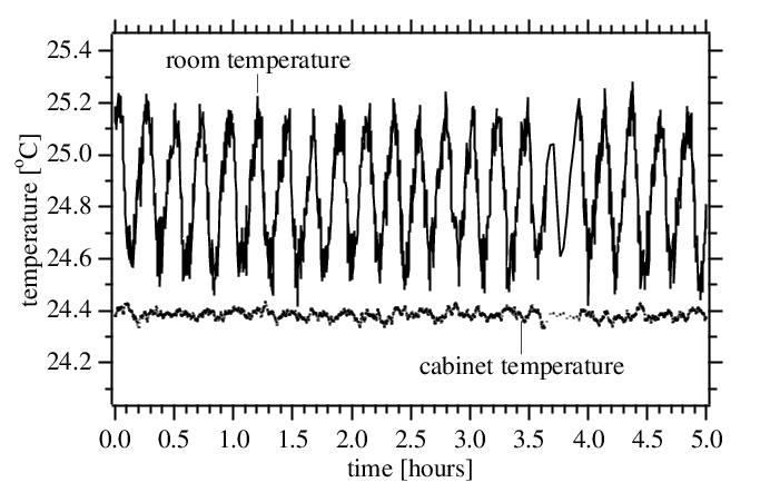
The maser resided in a closed, temperature stabilized room where the temperature oscillated with a peak-peak amplitude of slightly less than 0.5˚C with a period of around 15 minutes. The maser was contained in an insulated and thermally controlled cabinet, which provided a factor of five to ten shielding from the room, and reduced the fluctuations to less than 0.1˚C peak-peak, as shown in Fig. 14. By making large changes in the maser cabinet temperature and measuring the effect on the Zeeman frequency, we found a temperature coefficient of about 200 mHz/˚C. We believe this frequency shift was due mainly to the resistors which set the solenoid current, which had 100 ppm/˚C temperature coefficients. We monitored the cabinet temperature and placed a bound on the sidereal component of the temperature fluctuations at 0.5 mK, which would produce a systematic sidereal variation of 100 $\mu$ Hz on the Zeeman frequency, about a factor of 3 smaller than the measured limit on sidereal variation in Zeeman frequency.

As mentioned in Sec. III.3, spin-exchange effects induce a small offset of the Zeeman frequency given by Eqn. 23 from the actual Zeeman frequency [31]. This would imply that fluctuations in the input atomic flux (and therefore the maser power) could cause fluctuations in the Zeeman frequency measurement. We measured a limit on the shift of the Zeeman frequency due to large changes in average maser power at less than 0.8 mHz/fW. (Expected shifts from spin-exchange are ten times smaller than this level (Sec. III.3). We believe the measured limit is related to heating of the maser as the flux is increased). During long-term operation, the average maser power drifted approximately 1 fW/day (see Fig. 15). The sidereal component of the variations of the maser power were less than 0.05 fW, implying a variation in the Zeeman frequency of less than 40 $\mu$ Hz, an order of magnitude smaller than our experimental bound for sidereal Zeeman frequency variation.

V.3 Final result

We measured systematic errors in sidereal Zeeman frequency variation (as described in Secs. V.1 and V.2) due to ambient magnetic field (0.2 $\mu$ Hz), solenoid field (80 $\mu$ Hz), maser cabinet temperature (100 $\mu$ Hz), and hydrogen density induced spin-exchange shifts (40 $\mu$ Hz). Combining these errors in quadrature with the 0.34 mHz statistical uncertainty in Zeeman frequency variation, we find a sidereal variation of the $F=1$ , $\Delta m_{F}=\pm 1$ Zeeman frequency in hydrogen of 0.44 $\pm$ 0.37 mHz at the 1- $\sigma$ level. This 0.37 mHz bound corresponds to 1.5 $\times$ 10^-27 GeV in energy units.

VI Discussion

VI.1 Transformation to fixed frame

Our experimental bound of 0.37 mHz on sidereal variation of the hydrogen Zeeman frequency may be interpreted in terms of Eqn. 5 as a bound on vector and tensor components of the standard model extension. To make meaningful comparisons to other experiments, we transform our result into a fixed reference frame. Following the construction in reference [13], we label the fixed frame with coordinates (X,Y,Z) and the laboratory frame with coordinates (x,y,z), as shown in Fig. 16. We select the earth’s rotation axis as the fixed Z axis, (declination = 90 degrees). We then define fixed X as declination = right ascension = 0 degrees, and fixed Y as declination = 0 degrees, right ascension = 90 degrees. With this convention, the X and Y axes lie in the plane of the earth’s equator. Note that the $\alpha$ , $\beta$ axes of Sec. IV.5, also in the earth’s equatorial plane, are rotated about the earth’s rotation axis from the X,Y axes by an angle equivalent to the right ascension of 71^∘ 7’ longitude at 00:00 of November 19, 1999.

For our experiment, the quantization axis (which we denote z) was vertical in the lab frame, making an angle $\chi\approx$ 48 degrees relative to Z, accounted for by rotating the entire (x,y,z) system by $\chi$ about Y. The lab frame (x,y,z) rotates about Z by an angle $\Omega t$ , where $\Omega$ is the frequency of the earth’s (sidereal) rotation.

These two coordinate systems are related through the transformation

\left(\begin{array}[]{c}t\\ x\\ y\\ z\end{array}\right)=\left(\begin{array}[]{cccc}1&0&0&0\\ 0&\cos\chi\cos\Omega t&\cos\chi\sin\Omega t&-\sin\chi\\ 0&-\sin\Omega t&\cos\Omega t&0\\ 0&\sin\chi\cos\Omega t&\sin\chi\sin\Omega t&\cos\chi\end{array}\right)\left(\begin{array}[]{c}0\\ X\\ Y\\ Z\end{array}\right)=\mathbf{T}\left(\begin{array}[]{c}0\\ X\\ Y\\ Z\end{array}\right).

(28)

Then, vectors transform as $\vec{b}_{lab}={\mathbf{T}}\ \vec{b}_{fixed}$ , while tensors transform as ${\mathbf{d}}_{lab}={\mathbf{T}}\ {\mathbf{d}}_{fixed}{\mathbf{T}}^{-1}$ .

As shown in equation (5), our signal depends on the following combination of terms (for both electron and proton):

\tilde{b}_{3}=b_{3}-md_{30}-H_{12}.

(29)

Transforming these to the fixed frame, we see

$\displaystyle b_{3}$	$\displaystyle=$	$\displaystyle b_{Z}\cos\chi+b_{X}\sin\chi\cos\Omega t+b_{Y}\sin\chi\sin\Omega t,$
$\displaystyle d_{30}$	$\displaystyle=$	$\displaystyle d_{Z0}\cos\chi+d_{X0}\sin\chi\cos\Omega t+d_{Y0}\sin\chi\sin\Omega t,$	(30)
$\displaystyle H_{12}$	$\displaystyle=$	$\displaystyle H_{XY}\cos\chi+H_{YZ}\sin\chi\cos\Omega t+H_{ZX}\sin\chi\sin\Omega t,$

so our observable is given by

$\displaystyle\tilde{b}_{3}$	$\displaystyle=$	$\displaystyle\left(b_{Z}-md_{Z0}-H_{XY}\right)\cos\chi$	(31)
	$\displaystyle+$	$\displaystyle\left(b_{Y}-md_{Y0}-H_{ZX}\right)\sin\chi\sin\Omega t$
	$\displaystyle+$	$\displaystyle\left(b_{X}-md_{X0}-H_{YZ}\right)\sin\chi\cos\Omega t.$

The first term on the right is a constant offset, not bounded by our experiment. The second and third terms each vary at the sidereal frequency. Combining Eqn. 31 (for both e^- and p) with Eqn. 5, we see

	$\displaystyle\|\Delta\nu_{Z}\|^{2}$	$\displaystyle=$	$\displaystyle\left[\left(b_{Y}^{e}-m_{e}d_{Y0}^{e}-H_{ZX}^{e}\right)+\left(b_{Y}^{p}-m_{p}d_{Y0}^{p}-H_{ZX}^{p}\right)\right]^{2}\frac{\sin^{2}\chi}{h^{2}}$		(32)
		$\displaystyle+$	$\displaystyle\left[\left(b_{X}^{e}-m_{e}d_{X0}^{e}-H_{YZ}^{e}\right)+\left(b_{X}^{p}-m_{p}d_{X0}^{p}-H_{YZ}^{p}\right)\right]^{2}\frac{\sin^{2}\chi}{h^{2}}.$		(32)

Inserting $\chi$ = 48 degrees, we obtain the final result

\sqrt{\left(\tilde{b}_{X}^{e}+\tilde{b}_{X}^{p}\right)^{2}+\left(\tilde{b}_{Y}^{e}+\tilde{b}_{Y}^{p}\right)^{2}}=\left(3\pm 2\right)\times 10^{-27}\ GeV.

(33)

Our 1-sigma bound on Lorentz and CPT violation of the proton and electron is therefore 2 $\times$ 10^-27 GeV.

VI.2 Comparison to previous experiments

We compare our result with other recent tests of Lorentz and CPT symmetry in Table 3. Although our bounds are numerically similar to the those from the ¹⁹⁹Hg/¹³³Cs experiment, the simplicity of the hydrogen atom allows us to place bounds directly on the electron and proton; uncertainties in nuclear structure models do not complicate the interpretation of our result. The recent limit set by the torsion pendulum experiment of Adelberger et. al. [20] on electron Lorentz and CPT violation casts our result as a clean bound on Lorentz and CPT violation of the proton.

Experiment	$\tilde{b}_{X,Y}^{e}$ [GHz]	$\tilde{b}_{X,Y}^{p}$ [GHz]	$\tilde{b}_{X,Y}^{n}$ [GHz]
anomaly frequency of e^- in Penning trap [16]	$10^{-25}$	-	-
¹⁹⁹Hg and ¹³³Cs precession frequencies [22]	$10^{-27}$	$10^{-27}$	$10^{-30}$
this work [1]	$10^{-27}$	$10^{-27}$	-
spin polarized torsion pendulum [20]	$10^{-29}$	-	-
dual species ¹²⁹Xe/³He maser [21]	-	-	$10^{-31}$

Table 3: Electron, proton and neutron experimental bounds.

VI.3 Future work

To make a more sensitive measure of the sidereal variation of the Zeeman frequency in a hydrogen maser, it will be important to clearly identify and reduce the magnitude of the long term drifts of the Zeeman frequency. Possible sources of these drifts are magnetic fields near the maser bulb caused by stray currents in heaters or power supplies in the inner regions of the maser. Also, the scatter of the Zeeman data points, believed to be due mainly to residual thermal fluctuations, should be reduced. Both of these objectives could be accomplished by carefully rebuilding a hydrogen maser, with better engineered power and temperature control systems.

VII Acknowledgments

We gratefully acknowledge the encouragement of Alan Kostelecký. Financial support was provided by NASA grant NAG8-1434 and ONR grant N00014-99-1-0501. M.A.H. thanks NASA for fellowship support under the Graduate Student Researchers Program.

References

[1] D.F. Phillips, M.A. Humphrey, E.M. Mattison, R.E. Stoner, R.F.C. Vessot, and R.L. Walsworth, Phys. Rev. D, in press, (physics/0008230). See also (physics/0007062) and (physics/0007063).
[2] V.A. Kostelecky and S. Samuel, Phys. Rev. Lett. 63, 224 (1989).
[3] V.A. Kostelecky and S. Samuel, Phys. Rev. D 40, 1886 (1989).
[4] V.A. Kostelecky and S. Samuel, Phys. Rev. Lett. 66, 1811 (1991).
[5] V.A. Kostelecky and S. Samuel, Phys. Rev. D 39, 683 (1989).
[6] V.A. Kostelecky and R. Potting, Nucl. Phys. B 359, 545 (1991).
[7] V.A. Kostelecky and R. Potting, Phys. Lett. B 381, 89 (1996).
[8] V.A. Kostelecky, M. Perry, and R. Potting, Phys. Rev. Lett. 84, 4541 (2000).
[9] V.A. Kostelecky and R. Potting, in Gamma Ray-Neutrino Cosmology and Planck Scale Physics, edited by D.B. Cline (World Scientific, Singapore, 1993), see also (hepth/9211116).
[10] V.A. Kostelecky and R. Potting, Phys. Rev. D 51, 3923 (1995).
[11] D. Colladay and V.A. Kostelecky, Phys. Rev. D 55, 6760 (1997).
[12] D. Colladay and V.A. Kostelecky, Phys. Rev. D 58, 116002 (1998).
[13] V.A. Kostelecky and C.D. Lane, Phys. Rev. D 60, 116010 (1999).
[14] V.A. Kostelecky and C.D. Lane, J. Math. Phys. 40, 6245 (1999).
[15] R. Bluhm, V.A. Kostelecky, and N. Russell, Phys. Rev. Lett. 82, 2254 (1999).
[16] R.K. Mittleman, I.I. Ioannou, H.G. Dehmelt, and N. Russell, Phys. Rev. Lett. 83, 2116 (1999).
[17] H. Dehmelt, R. Mittleman, R.S. Van Dyck Jr., and P. Schwinberg, Phys. Rev. Lett. 83, 4694 (1999).
[18] E.G. Adelberger et al., in Physics Beyond the Standard Model, edited by P. Herczeg et al. (World Scientific, Singapore, 1999), p. 717.
[19] M.G. Harris, Ph.D. thesis, Univ. of Washington, 1998.
[20] B. Heckel, presented at the International Conference on Orbis Scientiae 1999, Fort Lauderdale, Florida, Dec., 1999.
[21] D. Bear, R.E. Stoner, R.L. Walsworth, V.A. Kostelecky, and C.D. Lane, Phys. Rev. Lett. 85, 5038 (2000).
[22] C.J. Berglund, L.R. Hunter, D. Krause Jr., E.O. Prigge, M.S. Ronfeldt, and S.K. Lamoreaux, Phys. Rev. Lett. 75, 1879 (1995).
[23] Gauge invariance and renormalizability exclude the parameters $e_{\nu}$ , $f_{\nu}$ , and $g_{\lambda\mu\nu}$ in the standard model extension. We therefore neglected them relative to the other terms.
[24] H.G. Andresen, Z. Phys. 210, 113 (1968).
[25] J. Vanier and C. Audoin, The Quantum Physics of Atomic Frequency Standards (Adam Hilger, Bristol, 1989), Chap. 6.
[26] D. Kleppner, H.M. Goldenberg, and N.F. Ramsey, Phys. Rev. 126, 603 (1962).
[27] D. Kleppner, H.C. Berg, S.B. Crampton, N.F. Ramsey, R.F.C. Vessot, H.P. Peters, and J. Vanier, Phys. Rev. 138, A 972 (1965).
[28] The maser used for our Lorentz symmetry test, maser P-28 was only temporarily available for our use, as it was in our lab only to undergo several repairs. As a result, the amount of data we could acquire was limited. Maser P-8 is housed permanently in our laboratory, so much of our characterization was done with this maser. However, this maser was not suitable for a Lorentz symmetry test because it suffered from large, long term Zeeman frequency drifts, attributed to less magnetic shielding and larger extraneous fields (e.g., from heating elements).
[29] E.M. Mattison, W. Shen, and R.F.C. Vessot, in Proceedings of the 39th Annual Frequency Contol Symposium (IEEE, New York, 1985), p. 72.
[30] N.F. Ramsey, Molecular Beams (Clarendon Press, Oxford, 1956), Chap. 2.
[31] J.-Y. Savard, G. Busca, S. Rovea, M. Desaintfuscien, and P. Petit, Can. J. Phys. 57, 904 (1979).
[32] M.A. Humphrey, D.F. Phillips, and R.L. Walsworth, Phys. Rev. A 62, 063405 (2000).
[33] P.L. Bender, Phys. Rev. 132, 2154 (1963).
[34] W.H. Press, S.A. Teukolsky, W.T. Vetterling, and B.P Flannery, Numerical Recipes in C, 2nd ed. (Cambridge University Press, Cambridge, 1988), p. 689.
[35] Had we chosen the slope discontinuity with maximum reduced chi square, the total sidereal amplitude for this run would have been 1.1 mHz $\pm$ 0.4 mHz.
[36] Philip R. Bevington and D. Keith Robinson, Data Reduction and Error Analysis for the Physical Sciences (McGraw Hill, New York, 1992), p. 64.
[37] R. Noble, Electronics and Wireless World, Sept. 1991, p. 726.