Systematic study of Coulomb distortion effects in exclusive (e,e′p) reactionsPreprint: SSF96-09-02
Abstract
A technique to deal with Coulomb electron distortions in the analysis of (e,e′p) reactions is presented. Thereby, no approximations are made. The suggested technique relies on a partial-wave expansion of the electron wave functions and a multipole decomposition of the electron and nuclear current in momentum space. In that way, we succeed in keeping the computational times within reasonable limits. This theoretical framework is used to calculate the quasielastic (e,e′p) reduced cross sections for proton knockout from the valence shells in 16O, 40Ca, 90Zr and 208Pb. The final-state interaction of the ejected proton with the residual nucleus is treated within an optical potential model. The role of electron distortion on the extracted spectroscopic factors is discussed.
pacs
21.10.Jx, 21.60.Jz, 24.10.Eq, 25.30.FjI Introduction
For a long time it has been recognized that the exclusive (e,e′N) reaction in the quasielastic (QE) region is a powerful tool for studying the single-particle motion inside the nucleus, and is a testing ground for the different available nuclear models. One of the principal interests in the exclusive (e,e′N) reaction is to extract the nucleon spectral function from the cross section. This spectral function can be interpreted as the joint probability to remove a nucleon with momentum from the target nucleus and to find the residual system at an excitation energy . Related to these spectral functions, spectroscopic factors and occupation numbers are often studied. They are a measure for the validity of the independent particle model (IPM). The spectroscopic factor gives the probability to reach the single-particle state specified by the quantumnumbers in the residual nucleus at an excitation energy . The occupation number gives the number of nucleons in the single-particle state in the target nucleus and involves an integration of the spectroscopic factors over the complete excitation energy range [1]. In the IPM the states above (under) the Fermi level are completely empty (filled) and the total hole (particle) strength is situated at a fixed single-particle energy. The deviation from full (no) occupancy for the orbits below (above) the Fermi level is a measure for correlations neglected in this mean-field approach.
The occupation probabilities in even-even nuclei have been calculated within several theoretical frameworks. Most models go beyond the mean-field approach and partially account for short- and/or long-range nucleon-nucleon correlations [1, 2, 3, 4, 5, 6]. Occupation probabilities for the single-particle states which considerably deviate from the IPM value were obtained. Moreover, it is demonstrated that the single-particle hole strength is fragmented over a broad range of energy. In particular, occupation numbers for the proton orbit in 208Pb have been calculated varying from [3] to [7] pointing towards a strong depletion of this hole state in the ground state of 208Pb. From an experimental point of view, the CERES method [8] was developed in an attempt to obtain absolute occupation numbers from experimental data. The model uses only relative spectroscopic factors and allows to account, in an approximate way, for the strengths at high missing energies, not accessible for experiment. With this method, the occupation number in 208Pb is found to be .
Although the advantages of the quasielastic (e,e′N) process to study spectroscopic factors are widely recognized, the extraction of these factors from experiment is still not free of ambiguities. For example, depending on the model used in the analysis of the 208Pb(e,e′p) reaction, the spectroscopic factor for the transition to the groundstate in 207Tl ( hole) varies from [9] to [10]. A reliable determination of spectroscopic factors requires an accurate knowledge of the (e,e′N) reaction mechanism (photoabsorption mechanism, final-state interaction (FSI) of the ejected nucleon with the residual nucleus) and the exact treatment of the Coulomb distortion of the scattered electrons, especially for heavy nuclei.
In this paper we present results from systematic calculations of (e,e′p) cross sections for a number of even-even target nuclei and various kinematical conditions and confront them with data taken at NIKHEF. The extracted spectroscopic factors are compared with the corresponding values deduced within other theoretical approaches [10, 11, 12, 13]. Much attention is paid to the effect of electron distortion on the calculated cross section. It is pointed out that, especially for scattering off heavy nuclei, an exact treatment of these effects is highly needed in order to reproduce the shape of the measured cross sections and, consequently, to obtain reliable spectroscopic factors.
This paper is organized as follows. In section II the theoretical formalism for the (e,e′N) reaction is outlined. The derivation of the cross section is divided in two subsections treating the electron and the nuclear aspect of the (e,e′N) reaction. The technical details are dealt with in appendix A. The numerical details of the adopted approach are discussed in section III. The formalism is applied to electro-induced one-proton knockout reactions from a number of medium-heavy target nuclei in section IV. Finally, some conclusions are drawn in section V.
II Formalism
II.1 Cross section
In this paper we describe the process in which an electron with four-momentum and spin polarization is scattered from a target nucleus at rest with a rest mass . The detected electron is characterized by its four-momentum and spin polarization . The energy transfer to the nucleus is supposed to be sufficient to eject a nucleon (proton or neutron) with four-momentum and spin projection out of the target nucleus leaving the residual nucleus with four-momentum . The differential cross section and the Feynman amplitude for this process are related as follows:
| (1) |
Throughout this paper we adopt natural and unrationalized Gaussian () units. In this relation stands for the separation energy of a nucleon out of the target nucleus and denotes the excitation energy of the residual nucleus. The rest masses of the ejected nucleon and the residual nucleus are given by and . The angles and specify the scattered electron and ejected nucleon with respect to the chosen reference frame. At this point this reference frame is not further specified. The sum implies a summation over all final states (electron and nuclear) and an average over the initial states (electron and nuclear). We only have to sum over these final states which satisfy the energy conservation relation.
In the Born approximation the transition amplitude can be written in terms of matrixelements of the electron and nuclear charge-current four-vector in momentum space in the following way:
| (2) |
The initial and final electron states are denoted by and . The target nucleus and final nuclear state consisting of a residual nucleus and an ejected nucleon are represented by and .
The Feynman amplitude can further be rewritten as follows
| (3) | |||||
The spherical components of the electron and nuclear current operators are taken with respect to the rotating reference frame (Fig. 1 (a)). In this way the third component of the current operator is directly related to the charge operator through the charge-current conservation relation.
II.2 The leptonic part
In this section we elaborate on the electron matrixelement in the expression for the Feynman amplitude. The relativistic electron charge-current operator in coordinate space reads
with the electron field operator in coordinate space. The initial and final electron wave functions are defined according to
| (7) | |||
| (8) |
and stand for four-dimensional Dirac spinors. They are solutions of the stationary electron Dirac equation:
| (9) |
where is the rest mass of the electron and is the scattering potential. The additional quantumnumber uniquely determines the electron wave function.
Dealing with high-energetic electrons the electron mass can be neglected with respect to its total energy and the Dirac equation can be written down in the ultrarelativistic limit . In the Dirac-Pauli representation for the and matrices and in the absence of an external potential the solutions of equation (9) are given by :
The spinors can be expressed in terms of the Pauli spinors and the matrixelements of the Wigner -matrix, i.e.,
| (13) |
The angles specify the momentum with respect to the chosen reference frame (). The Wigner matrix represents the rotation of the reference frame () over the Euler angles in the basis spanned by the eigenvectors of the operators and .
Assuming a central potential , the electron wave functions are evaluated by a phase shift analysis based on a partial-wave expansion. Indeed, the Dirac Hamiltonian commutes with the angular momentum operators and and with the operator but not with the orbital momentum operator . As such, we derived a complete set of operators with common eigenfunctions represented by :
We can construct the partial waves as follows:
We introduce the common notation
The spherical spin-orbit eigenspinor is defined in the following way
| (28) |
Each partial wave (II.2) can be easily proved to satisfy the eigenvalue equations (II.2) under the condition that the radial electron wave functions and are solutions of the following second-order differential equations:
For each partial wave the second-order differential equation for has to be solved numerically. For the regular solutions one imposes the following boundary conditions:
| (34) |
and one obtains the corresponding solution for through the relation:
| (35) |
The asymptotic behaviour of the radial electron wave functions for Coulomb potential scattering are given by ()
| (36) | |||||
| (37) |
The phase shift reflects the influence of the scattering potential . It consists of two parts, i.e., the Coulomb phase shift and an additional phase shift . For a Coulomb potential generated by the protons in the nucleus, the Coulomb phase shift is defined according to ():
| (38) |
Due to the fact that the scattering potential is spin-independent, one can easily verify that the total phase shift is -independent, i.e.,
| (39) |
Finally, the electron wave function is expanded in terms of these partial waves :
| (40) |
The initial and final electron wave functions have to satisfy the outgoing () respectively incoming () boundary conditions. Knowing the asymptotic behaviour of the radial electron wave functions, the coefficients are fixed by
| (41) |
At this point only the scattering potential remains to be specified. In general the central Coulomb scattering potential generated by protons is given by
| (42) |
with the nuclear charge density normalized according to . In the forthcoming discussion we have taken this charge density to correspond with a homogeneous spherical charge distribution of protons within the nuclear radius .
By switching off the scattering potential one can easily verify that the solution (40) coincides with the free electron wave function (II.2) since the differential equations (II.2) reduce to the differential equations for the spherical Bessel functions. In this way a sensitive testing case for our numerical approach is found.
We want to stress that the problem of Coulomb distortion of the initial and final electron in the electron scattering process is solved to all orders. Earlier work in this field by Boffi et al. [11] handled the electron distortion in an approximate way through a high-energy expansion of the electron wave functions combined with an expansion in powers of . The DWEEPY code [11] used in the analysis of the NIKHEF data adopts this approximate treatment of electron distortion. To lowest order in it was proved that electron distortion effects could be approximated by an effective momentum approach (EMA). This means that the plane wave in eq. (II.2) has to be replaced by
| (43) |
with
| (44) |
Clearly this approach is very easy to handle and worth comparing with the complete distorted wave approach so that its degree of accuracy can be estimated.
II.3 The nuclear part
In a previous paper [14], we have shown that at low values of the missing momentum, meson-exchange currents (MEC) and long-range effects only slightly affect the calculated (e,e′p) cross section. As we will restrict ourselves to QE (e,e′p) reactions at low missing momenta only the one-body part of the nuclear four-current is retained. Hereby we adopt the operator as dictated in the non-relativistic impulse approximation:
| (45) | |||||
This nuclear charge-current four-vector refers to non-interacting point-like nucleons with mass . To correct for the finite extent of the nucleons, the Sachs electromagnetic formfactors and are introduced.
As for the electron wave functions, the final nuclear wave function is determined through a phase shift analysis after an expansion in partial waves. The final nuclear state is taken to be a linear combination of one particle-one hole excitations out of the A-particle groundstate with . The hole state is characterized by the quantumnumbers and energy . The continuum particle state is specified by the quantumnumbers and the energy . The isospin nature of the particle-hole state is denoted by . The particle-hole state in the coupled scheme is defined according to
| (46) |
with the uncoupled particle-hole state defined as follows
| (47) |
and . The operators and denote single-particle creation and annihilation operators. The radial wave functions for the bound hole states are solutions of the Schrödinger equation with a Hartree-Fock potential generated with an effective interaction of the Skyrme type (SkE2) [15]. The continuum particle states are evaluated within an optical potential model (OPM) [11]. The physical radial wave functions are regular in the origin and behave asymptotically according to
where and the momentum stand for
The complex phase shifts caused by the nuclear and Coulomb part of the optical potential are denoted by and ().
Given the asymptotic behaviour for the radial single-particle wave functions and imposing that the ejected nucleon wave function satisfies the incoming boundary conditions, the final nuclear state is given by
| (55) | |||||
In order to derive this expression the target nucleus is considered to be a spherical nucleus in the groundstate. In addition, the residual nucleus is described by a pure hole state with respect to this target nucleus groundstate.
II.4 The Feynman amplitude
As the initial and final electron wave function and the final nuclear state are expanded in partial waves, it is common to decompose the electron and nuclear charge-current operators in the Coulomb, Electric and Magnetic multipole operators of rank ():
| (56) |
with the vector spherical harmonics defined according to
| (57) |
and the standard spherical unit vectors corresponding with the unit vectors () in the reference frame (Fig. 1 (a)).
Accordingly, in momentum space the charge-current operators can be written as:
| (58) |
with and the Euler angles defined in Fig. 1 (a).
It is well-known that when neglecting electron distortion effects, the differential (e,e′N) cross section can be written in terms of four structure functions containing all the nuclear information. In such a Distorted Wave Born Approximation (DWBA) approach each structure function is multiplied with an analytical factor containing the leptonic information. This is no longer valid in the Coulomb Distorted Wave Born Approximation (CDWBA) approach as the electron part can no longer be separated from the nuclear part. Consequently, when accounting for Coulomb distortion effects one has to perform a multipole expansion for both the electron and nuclear charge-current operators.
Combining equations (3) and (II.4) and applying some basic properties of the Wigner matrices the Feynman amplitude reads as ()
| (59) | |||||
The superscript and refer to the electron and the nuclear multipole operators. We have deliberately chosen to work out the leptonic and nuclear matrixelements in momentum space. Earlier electron distortion calculations by Jin et al. [10] and Udías et al. [12] evaluate the transition matrixelements in coordinate space. In order to make their calculations feasible the nucleon formfactors are evaluated at the asymptotic value . The major advantage of our approach is that the momentum-dependence of the nucleon formfactors can be handled exactly.
Here we will solely calculate the unpolarized (e,e′N) cross section (1) so we need to evaluate
| (60) |
The summation over the initial and final states involves a sum over the initial and final electron polarizations and a sum over the polarizations of the recoiling nucleus and the ejected nucleon. In appendix A this Feynman amplitude is further worked out. Summarizing from appendix A, one can state that the calculation of the (e,e′N) cross section is reduced to the evaluation of a large number of leptonic radial integrals and a set of reduced transition matrixelements containing all nuclear information. We stress that the technique developed here can be easily extended to polarization processes.
III Numerical procedure
In order to derive the exclusive (e,e′p) cross section (1) in the CDWBA we need to evaluate the Feynman amplitude discussed in the previous section and appendix A. The numerical procedure is schematically sketched in Fig. 2. From a numerical point of view the evaluation of this transition amplitude is cumbersome as it involves an integration over the complete range and two infinite sums, i.e., the sum over the different multipolarities in the multipole expansion of the leptonic and hadronic current and the sum over the angular momentum originating from the partial-wave expansion of the scattered electron state. Angular momentum selection rules make sure that the other summations in the equations (A) and (A) have a finite range for fixed values of and .
When accounting for electron distortion effects, the integrandum in the integral over peaks at the effective momentum transfer . As the EMA is only an approximation of electron distortion effects the integrandum is spread around this value and the integration in -space has to be performed in an interval around . It is worth noting that in the absence of electron distortion effects, the integral over vanishes and the standard DWBA expressions are retained. The integrandum then reduces to a -function representing the momentum conservation relation .
The finite extent of the nucleus puts a constraint on the number of multipolarities which have to be retained in the multipole expansion of the nuclear current given in eq. (II.4). In the calculations we systematically observe convergence when including multipolarities up to where denotes the radius of the considered target nucleus. In a similar way the number of electron partial waves which contribute to the (e,e′p) cross section, is restricted by an upper limit . It can be easily verified that the electron partial waves and corresponding with large values for are negligible for values of within the nucleus range. For that reason, these electrons can cause no nuclear transitions. Consequently, to a required accuracy, only a finite number of the electron partial waves contributes to the electron scattering cross section. The number of electron partial waves actually contributing to the cross section depends also on the electron energy. The higher the electron energy the more partial waves will be required. The numerical evaluation of the (e,e′p) cross sections is getting complicated due to the large number of electron partial waves to consider. This is a result of the long-range character of the Coulomb interaction. The limit (equivalent with turning off the electron distortions) can be considered as a severe test of the accuracy of the numerical techniques and a convergence test for the electron partial waves. For , the electron wave functions reduce to plane waves. Accordingly, the DWBA cross section should be retained. As will be demonstrated in the forthcoming sections, our code has been checked to comply with this requirement.
Another important feature of our CDWBA approach is that the radial integrals (), which are the heart of our numerical procedure, do not depend on the scattering angles and . Consequently, our numerical procedure is optimized for calculating the (e,e′p) cross section for these specific kinematical conditions where the electron and proton scattering angles are varied and the other electron characteristics are kept fixed. The complete missing momentum range of the (e,e′p) cross section for proton knockout from the different hole states can then be calculated with a stored set of radial integrals.
IV Results
Up to now, most of the high-resolution (e,e′p) experiments performed at NIKHEF (Amsterdam), Saclay, Mainz and MIT-Bates have been carried out by using either parallel or constant kinematics. Both correspond with in-plane experiments: the ejected proton is detected in the scattering plane spanned by the initial and final electron. In parallel kinematics the proton is detected in the direction of the momentum transfer. By varying the incoming and outgoing electron energies or/and the scattering angle , different values for the momentum transfer and consequently the missing momentum are reached. For constant kinematics the energy-momentum transfer is kept fixed and the proton angular distribution is measured. The missing momentum is defined positive when the ejected proton lies in the half-plane of the initial electron momentum and bordered by the momentum transfer. In the other half-plane the missing momentum is negative.
Most of the experimental data are presented in terms of the reduced cross section extracted from the measured cross section in the following way (, )
| (61) |
with the off-shell electron-proton cross section. We stress that only in the plane-wave impulse approximation (PWIA) the reduced cross section coincides with the nucleon spectral function , i.e., the probability to eject a nucleon with momentum from the target nucleus while leaving the residual nucleus at an excitation energy . As soon as the FSI, electron distortion and many-body nuclear currents effects come into play this quantity can no longer be interpreted as the nucleon spectral function. In comparing our (e,e′p) results with the available data we have divided the calculated cross sections with the prescription [16] for . The same procedure was applied to the experimental cross sections presented in this paper. Moreover, the calculated curves are scaled with a spectroscopic factor which accounts for the fragmentation of the single-particle strength.
The results of our model calculation are compared with the predictions from three other model calculations. Firstly, we confront our results with the non-relativistic CDWBA model of Boffi et al.[11]. This model is at the basis of the DWEEPY code often used in the analysis of the NIKHEF (e,e′p) data. In the latter model the FSI is treated in a non-relativistic optical potential calculation similar to ours. In contrast with our model, the bound state wave functions are calculated in a Wood-Saxon well. The rms radius of the bound state wave function is fitted to reproduce the shape of the measured reduced cross section and the well depth is adjusted to reproduce the experimentally observed separation energy. In our calculation, we use the bound state wave functions as obtained from a Hartree-Fock calculation with a density-dependent effective interaction. Accordingly, in our approach the spectroscopic factor is the only parameter adjusted to the data. Concerning the treatment of electron distortion effects the two models are very different. Whereas in our calculation Coulomb electron distortion effects are treated to all orders, the CDWBA model of Boffi et al. implements electron distortion effects within the high-energy expansion as briefly mentioned in the theoretical discussion of section II.2. In comparing the results obtained with these two non-relativistic models one can study in how far an exact treatment of electron distortion effects is required in the analysis of (e,e′p) reactions.
Our results for the reduced cross sections and the corresponding spectroscopic factors are also confronted with the completely relativistic calculations of Jin et al. [10] and Udías et al. [12]. In line with our approach, the two models handle the electron distortion in an exact distorted wave calculation. The main difference with our model occurs in the description of the photoabsorption process and the initial and final nuclear system in the (e,e′p) process. Jin et al. and Udías et al. work in a totally relativistic framework. The bound state wave functions are calculated from the Dirac equation with a scalar and vector potential which are parametrized fits to relativistic Hartree potentials. The wave function of the knocked out nucleon is the solution of the Dirac equation with a relativistic optical potential. Two different prescriptions for the relativistic nuclear current operator are considered. They are referred to as the and current operators and follow the conventions of ref. [16].
IV.1 Parallel kinematics
In this section we deal with the quasielastic (e,e′p) reaction from 16O, 40Ca, 90Zr and 208Pb in parallel kinematics. In Table 1 we specify the studied kinematical conditions. They all correspond with measurements performed at the NIKHEF electron accelerator. The (e,e′p) cross section for these different target nuclei are calculated in the CDWBA framework as outlined in the previous sections. The FSI of the ejected proton with the residual nucleus is handled within an OPM. For the medium-heavy nuclei 40Ca, 90Zr and 208Pb the potential as derived from the Schwandt parameterization [22] is considered. This optical potential is known to provide a good description of the elastic (p,p′) scattering data over a large range of target mass and incident proton energies. The target nucleus 16O is out of the range of nuclei used in the parameterization of this global optical potential. Therefore, for the 16O(e,e′p) calculations, we adopt the optical potential which is directly extracted from a recent analysis of elastic 16O(p,p′) scattering data at MeV and use the parameterization quoted as ”WS” in ref. [17]. In order to study the effect of Coulomb distortions the (e,e′p) predictions from the DWBA and CDWBA model are compared. We stress that these two models only differ in the way the Coulomb distortions are described. In the DWBA they are completely neglected, whereas in the CDWBA they are treated exactly.
The CDWBA reduced cross sections for electro-induced proton knockout from the and shell in 16O are confronted with the NIKHEF data in Fig. 3. The DWBA and CDWBA curves for each state are multiplied with one and the same spectroscopic factor. This spectroscopic factor is extracted from a least-square fit of the CDWBA reduced cross section to the data. The multiplication factors as extracted from our calculation adopting the WS optical potential are given in Table 2. Table 2 also lists the spectroscopic factors obtained within the non-relativistic CDWBA model of the Pavia group [11] as reported in ref. [17]. Comparing the results presented in this work and the predictions outlined in ref. [17], a similar degree of agreement with the data is reached. The extracted spectroscopic factors agree within . From Fig. 3 it is clearly seen that the calculated reduced cross sections reproduce the measurements very well and electron distortion effects, although small, improve the agreement with the data especially for knockout from the orbit in 16O.
We also performed calculations for electro-induced one-proton knockout from the and shell in 40Ca. The results are plotted in Fig. 4. Electron distortion effects seem to follow the same pattern as observed for electron scattering from 16O, but the effect is now more pronounced. From the 16O(e,e′p) and 40Ca(e,e′p) results one can already trace the main effects of electron distortion on the reduced cross section in parallel kinematics:
- •
Electron distortion shifts the reduced cross section towards higher missing momenta. This can be explained by considering that a virtual photon exchanged between the electron and the nucleus will carry a momentum instead of (). From equation (44) and the definition of one deduces that this shift will be decreasing with increasing .
- •
The shape of the reduced cross section is mainly modified at the minima and maxima. Clearly, electron distortion not only manifests itself in an effective momentum shift but also in a focusing effect of the electron beam onto the target nucleus.
The curves in Fig. 4 are scaled with a spectroscopic factor obtained from a least-square fit of the CDWBA results to the data. In Table 3 we compare the spectroscopic factors from our analysis with those obtained from the non-relativistic analysis with the DWEEPY code [11] and those extracted from the two complete relativistic calculations by Jin et al. [10] and Udías et al. [12].
Comparing the spectroscopic factors for proton knockout from the shell two main features can be observed:
- •
The spectroscopic factors obtained with the non-relativistic models are in very good agreement with each other but are considerably smaller than the relativistic values obtained with the nuclear current operator;
- •
The spectroscopic factors extracted within the relativistic models seem to be very sensitive to the prescription for the off-shell nuclear current operator. The current operator results in a spectroscopic factor for the state that differs with more than from the result. The current operator is obtained from the current operator using the Gordon decomposition and should produce similar results for on-shell nucleons.
The appreciable difference between the relativistic and non-relativistic approaches is rather surprising considering that the proton kinetic energies dealt with are typically of the order of MeV. According to Jin et al. [23] and Udías et al. [12, 24] the noticeable difference between the relativistic and non-relativistic spectroscopic factors is caused by the stronger absorptive part in the relativistic potentials. Even though all optical potentials reproduce the elastic proton-nucleus scattering data to a more or less similar degree, the quenching of the reduced cross section due to the final-state interaction of the ejected proton with the residual nucleus can differ by adopting a relativistic or non-relativistic optical potential. This can be attributed to the behaviour of the optical potential in the nuclear interior. One could however doubt whether the interior part of the optical potential can be constrained in elastic proton scattering processes that are typical surface events.
Hedayati-Poor et al. [25] attribute the difference between the relativistic and non-relativistic spectroscopic factors to the nuclear current operator. They show that the non-relativistic reduction of the relativistic transition amplitude results in an effective non-relativistic current operator which depends on the strong scalar and vector potentials [26] for the bound and the continuum single-particle states. Instead of using this medium-modified non-relativistic nuclear current, we adopt the standard non-relativistic nuclear current operator in our calculations. In our opinion, this is justified as long as the sensitivity of the relativistic results to the choice of the relativistic nuclear current operator is not cleared up.
Concerning the spectroscopic factors obtained for proton knockout from the shell (see Table 3), the different models give very different predictions. In conformity with the calculation of Udías et al. we describe rather poorly the reduced cross section around , especially in the negative missing momentum region. This results in a spectroscopic factor which is not very reliable. However it has to be stressed that, in contrast with what was done in the analysis of ref. [18], no attempt has been made to improve the results by adjusting the parameters of the optical potential and/or by adjusting the bound-state wave characteristics (rms radii and binding energies).
The next target nucleus we considered is 90Zr. The calculations cover knockout from the different valence shells in 90Zr for two different proton kinetic energies ( and MeV). We investigate to what extent the reduced cross sections for knockout from the outermost shells (2p1/2, 2p3/2, 1f5/2) are affected by electron Coulomb distortion effects. Secondly the results of the complete calculation are confronted with the available data. In Fig. 5 the reduced cross sections derived within the DWBA (neglecting electron distortion) and the complete CDWBA framework are compared with the predictions adopting the EMA.
The gross features which were pointed out in the previous sections again show up. For the two proton kinetic energies, electron distortion shifts the reduced cross section towards higher missing momenta. However this shift is less pronounced in the CDWBA calculation than in the EMA approach. In Table 5 we list the missing momenta corresponding with the first maxima in the reduced cross section for knockout from the orbit for the different steps in the formalism. We remark a general behaviour for the two proton kinetic energies. Including FSI effects which is equivalent with going from a PWIA to a DWBA approach, a shift towards lower is noticed. This shift, opposite to the shift due to electron distortion, can be easily explained on the basis of an effective proton momentum. The ejected proton feels an attractive potential (real part of the optical potential) which causes the detected proton to have a smaller asymptotic momentum than the momentum of the initially struck proton. Table 5 also shows that this shift towards lower is increasing with decreasing proton energy. The latter is easily explained as the real part of the optical potential induces a shift in the average measured proton momentum approximately given by [11]
| (62) |
where is the average value of the real part of the optical potential over the interaction region.
The inclusion of electron distortion effects in the model shifts the reduced cross section towards higher . The shift obtained from the EMA is larger for MeV than for MeV since for the latter the reduced cross section at the peak position corresponds with a smaller momentum transfer. The complete CDWBA calculation produces more than just a shift towards higher . The focusing of the electron beam in the vicinity of the target nucleus strongly modifies the maxima and minima of the reduced cross section with respect to the DWBA results. Since the extracted spectroscopic factors are sensitive to the behaviour of the reduced cross section at the peaks, an accurate prediction of this focusing effect is extremely important for an accurate deduction of these quantities.
In Fig. 6 the CDWBA results are confronted with the data. The different curves are multiplied with the spectroscopic factors that are determined from the MeV data (Table 4). Firstly, it is clear that for MeV the calculated cross sections are in very good agreement with the data. On the other hand, for the MeV data the shape of the measured reduced cross sections is not well reproduced by the CDWBA calculations and, as such, the extracted spectroscopic factors can not be considered as reliable. This conclusion agrees with the findings of den Herder in ref. [20]. In ref. [20] it was shown that a slight reduction of the depth of the central imaginary part of the optical potential resulted in a much better agreement with the data for MeV. With this modified optical potential an equally good fit of the elastic proton scattering data was obtained. This indicates that low energy (p,p′) reactions are rather insensitive to the depth of the imaginary part in the nuclear interior. The (e,e′p) results, however, are sensitive to this part of the optical potential. The second maximum in the reduced cross section reflects the behaviour of the single-particle wave function in the nuclear interior. Since the overlap is taken with the continuum wave functions, the second maximum is sensitive to the shape of the continuum wave function in the nuclear interior. Given the uncertainties in the optical potential, this behaviour is not very accurately determined. As the single-particle wave function is more surface peaked, this also explains why the reduced cross section is not that sensitive to the depth of the imaginary part of the optical potential. Clearly, the sensitivity of the reduced cross section to the parameterization of the optical potential is a general weakness of CDWBA models but does not affect the general conclusions with respect to the role of electron distortion on the reduced cross section.
The spectroscopic factors extracted from our 90Zr(e,e′p) calculation are systematically larger than the values obtained by den Herder [20]. This deviation can be partly attributed to the fact that in ref. [20] a different optical potential is considered. Furthermore, the analysis performed by den Herder accounts for electron distortion effects in an approximate way, thus overestimating the focusing effect of the electron beam.
The electro-induced one-proton knockout reaction from 208Pb is the ultimate testing case to study electron distortion effects. The 82 protons in 208Pb generate a strong Coulomb potential felt by the initial and final electron. We have calculated the 208Pb(e,e′p) reduced cross sections for proton emission from the , , , and shells.
As the effect of Coulomb distortions increases with proton number , we consider 208Pb the ideal target nucleus to illustrate the numerical accuracy of our technique. The convergence rate for the electron partial waves is illustrated in Fig. 7. Convergence is reached for and the code is verified to produce gradually converging results, which is not evident, considering the large number of partial waves that has to be considered. The convergence tests were performed with electron wave functions of the spherical Bessel type. Accordingly, when convergence is reached the resulting cross section should coincide with the one obtained in a DWBA approach, provided that similar model assumptions with respect to the bound state wave functions and the FSI are adopted. In the insert of Fig. 7 it is verified that our CDWBA code bears this thorough test.
Fig. 8 shows a comparison of the CDWBA reduced cross sections with the DWBA and EMA results. All curves are multiplied with the spectroscopic factors as listed in Table 6. The spectroscopic factors are derived from a best fit of the CDWBA curve to the data. The data are well reproduced in the CDWBA, especially for the positive side. We remark that electron distortion effects considerably improve on the agreement with the data. Besides a shift towards higher , the minima and the maxima of the DWBA reduced cross section are strongly modified when including electron distortion effects in the model.
In Table 7 some characteristics of the first and second maximum of the reduced cross section are listed. The numbers clearly demonstrate that the final-state interaction of the ejected nucleon with the residual nucleus causes a small shift of the reduced cross section towards higher . Electron distortion effects also show up in a shift towards higher . The EMA again overestimates this feature compared with the complete distorted wave calculation. Moreover, in the CDWBA model, the shift in related to electron distortion is more pronounced for the first than for the second peak. This can be easily understood by considering that the two peaks in the reduced cross section correspond with different values for the momentum transfer . The focusing of the electron beam onto the target nucleus is reflected in an enhancement of the cross section at the peak positions with respect to the EMA cross section. The relativistic calculation by Udías et al. [12] predicts a relative enhancement which is somewhat larger than our estimate. Nevertheless, it is clear that the two complete distorted wave calculations do not reproduce the strong focusing effect of electron distortion as observed with the DWEEPY code [28, 29]. The CDWBA model of the Pavia group predicts an enhancement for the first peak in the reduced cross section of about due to the focusing of the electron beam onto the nucleus. This model accounts for electron distortion effects up to second order in the high-energy approximation. It has to be stressed that apart from the treatment of electron distortion effects, the Pavia and our model are very similar. Accordingly, the procedure of treating electron distortion effects is the only plausible explanation for the considerably different spectroscopic factors extracted with the two models.
Summarizing, the effect of Coulomb distortion in parallel kinematics can be understood in terms of a shift of the reduced cross section towards higher and a small enhancement of the reduced cross section due to the focusing of the electron beam onto the nucleus. It is also demonstrated that electron distortion effects become more important for heavier nuclei and need to be treated in a complete distorted wave calculation in order to extract reliable spectroscopic factors.
IV.2 Constant kinematics
We find that for constant kinematics electron distortion effects act in a different way than for parallel kinematics. This is illustrated in Fig. 9 where we investigate electro-induced proton knockout from the shell in 208Pb for quasielastic kinematics (). In this calculation, the electron energy is the same as the one for the parallel kinematics case considered in the previous section. The EMA no longer causes a shift of the reduced cross section towards higher but now results in a strong quenching of the reduced cross section around . The peak of the reduced cross section at in Fig. 9 coincides with the reduced cross section for parallel kinematics at displayed in Fig. 8. Moreover, the reduced cross section in parallel kinematics around shows a strong dependence on , i.e., the slightest modification of considerably affects the value for the reduced cross section. Consequently, a different prescription of than the one extracted from eq. (44) can cause a considerable modification of the EMA reduced cross section at for constant kinematics.
In going from the EMA to the CDWBA, a strong enhancement of the reduced cross section around MeV/c is observed. From the previous considerations, this can be ascribed to a smaller -value than the one adopted in the EMA approach and the focusing effect of the electron beam onto the nucleus. For constant kinematics it is therefore more difficult to disentangle the different contributions from electron distortion as the momentum transfer shift and the focusing effect both might cause either an enhancement or quenching of the reduced cross section.
In order to give a complete picture of the role of Coulomb distortion on the exclusive (e,e′p) reaction, the 208Pb reduced cross section for constant kinematics is also studied for non-quasielastic kinematics. Two different kinematics are considered, one in the low- () and one in the high-energy () side of the quasielastic peak. The results are plotted in Fig. 10.
The reduced cross sections show a specific pattern regarding electron distortion effects. The DWBA results are shifted towards higher (lower) missing momenta for (). This feature can be easily explained within the EMA. We stress that this EMA shift is only a first estimate of the role of electron distortion on the exclusive (e,e′p) reduced cross section for non-quasielastic kinematics. It is clear from Fig. 10 that a complete distorted wave calculation is required to completely account for electron distortion effects.
V Conclusions
We have analyzed the quasielastic (e,e′p) reaction from various target nuclei. A technique is presented to deal with Coulomb distortion effects in an exact manner keeping the computational time within reasonable limits. We presented results for reduced cross sections as a function of missing momentum, corresponding to proton knockout from the outermost shells in 16O, 40Ca, 90Zr and 208Pb considering two different types of kinematical arrangements.
For parallel kinematics, Coulomb electron distortion causes a shift of the cross section towards higher missing momenta. This shift can be partially reproduced by the use of an effective momentum transfer. Furthermore,the focusing effect of the electron beam onto the nucleus mainly affects the maxima and minima of the reduced cross section. It has been shown that in order to extract realistic spectroscopic factors an accurate determination of this effect is highly needed.
The role of electron distortion in the (e,e′p) reaction for constant kinematics was investigated on the basis of the one-proton knockout reaction from the shell in 208Pb. For quasielastic kinematics the focusing effect and the effective momentum transfer effect caused by Coulomb electron distortion are reflected in an enhancement, respectively, quenching of the DWBA reduced cross section around . For non-quasielastic kinematics, electron distortion effects cause a shift of the DWBA reduced cross section towards higher or lower missing momentum depending if we probe the high- or low-energy side of the quasielastic peak.
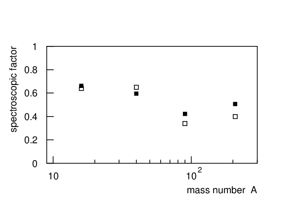
The spectroscopic factors extracted in our model agree within with the corresponding spectroscopic factors derived from an analysis applying the CDWBA code of the Pavia group. As can be seen from Fig. 11, we mostly obtain larger values. This can be partially attributed to the way of treating electron distortion effects. The approximate treatment of electron distortion by the Pavia group [11] tends to overestimate the focusing effect of the electron beam onto the nucleus and produces in this way smaller spectroscopic factors than our values.
Acknowledgment
This work has been supported by the Fund for Scientific Research - Flanders (FWO).
Appendix A Feynman amplitude in the CDWBA
In this appendix we work out the CDWBA feynman amplitude (60) for the electro-induced one-nucleon knockout process. Combining eqs. (II.4) and (59) with the expressions for the electron charge-current four-vector (II.2), the distorted electron wave functions (40) and the distorted nuclear wave function (55) and applying some basic properties of the Wigner matrices, the summation (60) can be rewritten as
| (63) |
with
| (64) | |||||
For the derivation of this expression we have chosen the reference frame and the electron and nucleon scattering angles according to the definitions fixed in Fig. 1(b).
The electron part reads as
The radial integrals in this expression are evaluated in the following way
where stands for in the Coulomb and electric radial integrals and for in the magnetic radial integrals. It can easily be verified that in case satisfy even (odd) than satisfy even (odd). Moreover, can be evaluated with either of the two choices () or () since for both sets the same result is obtained. The initial and final radial electron partial waves occur in the expressions for the radial integrals given by
| (80) | |||||
| (81) | |||||
| (82) | |||||
The following reduced matrixelements are useful in the evaluation of these integrals
The nuclear part in eq. (64) is written in terms of the reduced matrixelements , and defined as follows:
| (93) |
We get
At this stage we described the (e,e′N) process in its most general form. All approximations with respect to the photoabsorption mechanism and the final-state interaction (FSI) of the ejected nucleon with the nucleus are contained in the matrixelements , and . Moreover, besides the fact that we consider the ultrarelativistic limit, electron distortion effects are accounted for exactly. For the one-body nuclear current operator of the impulse approximation (45), these reduced matrixelements are evaluated in ref. [30].
References
- [1] C. Mahaux, P.F. Bortignon, R.A. Broglia and C.H. Dasso, Phys. Rep. 120, 1 (1985).
- [2] D. Van Neck, M. Waroquier and J. Ryckebusch, Nucl. Phys. A530, 347 (1991).
- [3] V.R. Pandharipande, C.N. Papanicolas and J. Wambach, Phys. Rev. Lett. 53, 1133 (1984).
- [4] H. Müther, A. Polls and W.H. Dickhoff, Phys. Rev. C 51, 3040 (1995).
- [5] H. Müther and L.D. Skouras, Nucl. Phys. A581, 247 (1995).
- [6] A. Polls, H. Müther and W.H. Dickhoff, Nucl. Phys. A594, 117 (1995).
- [7] C. Mahaux and R. Sartor, Adv. Nucl. Phys. 20, 1 (1991).
- [8] P. Grabmayr, Prog. Part. Nucl. Phys. 29, 251 (1992).
- [9] E.N.M. Quint, PhD-thesis, University of Amsterdam, 1988.
- [10] Y. Jin, D.S. Onley, L.E. Wright, Phys. Rev. C 45, 1311 (1992).
- [11] S. Boffi, C. Giusti and F.D. Pacati, Phys. Rep. 226, 1 (1993).
- [12] J.M. Udías, P. Sarriguren, E. Moya de Guerra, E. Garrido and J.A. Caballero, Phys. Rev. C 48, 2731 (1993).
- [13] Y. Jin, PhD-thesis, Ohio University, 1991.
- [14] V. Van der Sluys, J. Ryckebusch and M. Waroquier, Phys. Rev. C 54, 1322 (1996).
- [15] M. Waroquier, J. Ryckebusch, J. Moreau, K. Heyde, N. Blasi, S.Y. van der Werf and G. Wenes, Phys. Rep. 148, 249 (1987).
- [16] T.D. DeForest, Jr., Nucl. Phys. A392, 232 (1983).
- [17] M. Leuschner et al., Phys. Rev. C 49, 955 (1994).
- [18] G.J. Kramer et al., Phys. Lett. B 227, 199 (1989).
- [19] G.J. Kramer, PhD-thesis, University of Amsterdam, 1990.
- [20] J.W.A. den Herder, PhD-thesis, University of Amsterdam, 1987.
- [21] J.W.A. den Herder, P.C. Dunn, E. Jans, P.H.M. Keizer, L. Lapíkas, E.N.M. Quint, P.K.A. De Witt Huberts, H.P. Blok, G. Van der Steenhoven, Phys. Lett. B 161, 65 (1985).
- [22] P. Schwandt, H.O. Mayer, W.W. Jacobs, A.D. Bacher, S.E. Vigdor and M.D. Kaitchuk, Phys. Rev. C 26, 55 (1982).
- [23] Y. Jin and D.S. Onley, Phys. Rev. C 50, 377 (1994).
- [24] J.M. Udías, P. Sarriguren, E. Moya de Guerra, E. Garrido and J.A. Caballero, Phys. Rev. C 51, 3246 (1995).
- [25] M. Hedayati-Poor, J.I. Johansson, H.S. Sherif, Phys. Rev. C 51, 2044 (1995).
- [26] J.D. Walecka, Ann. of. Phys. (NY) 83, 491 (1974).
- [27] J.M. Udías, P. Sarriguren, E. Moya de Guerra and J.A. Caballero, Phys. Rev. C 53, R1488 (1996).
- [28] C. Giusti and F.D. Pacati, Nucl. Phys. A473, 717 (1987).
- [29] C. Giusti and F.D. Pacati, Nucl. Phys. A485, 461 (1988).
- [30] J. Ryckebusch, M. Waroquier, K. Heyde, J. Moreau and D. Ryckbosch, Nucl. Phys. A476, 237 (1988).
| (MeV) | (MeV) | (MeV/c) | |
|---|---|---|---|
| 16O(e,e′p) (a) | 455.8 | 115 | -177 …265 |
| 40Ca(e,e′p) (b) | 460 | 114 | -225 …285 |
| 90Zr(e,e′p) (c) | 346.5 | 81 | 27 …168 |
| 90Zr(e,e′p) (c) | 350.7 | 114 | 62 …298 |
| 208Pb(e,e′p) (d) | 412.3 | 113 | -50 …300 |
| (MeV) | CDWBA (this work) | CDWBA(a) | |
|---|---|---|---|
| 0 | 0.66 | 0.64 | |
| 6.3 | 0.54 | 0.51 |
(a) ref. [17]
| (MeV) | CDWBA (this work) | CDWBA(a) | rel. CDWBA(b) | rel. CDWBA(c) | |
|---|---|---|---|---|---|
| 0 | 0.60 | 0.65 | 0.80 | 0.76 (0.60) | |
| 2.522 | 0.48 | 0.51 | 0.75 | 0.51(0.44) |
| (MeV) | CDWBA (this work) | CDWBA (this work) | CDWBA(a) | |
| ( MeV) | ( MeV) | |||
| 0 | 0.42 | 0.31 | 0.34 | |
| 1.507 | 0.51 | 0.36 | 0.44 | |
| 1.745 | 0.52 | 0.44 | 0.33 |
(a) ref. [20]
| (MeV/c) | (MeV/c) | |
|---|---|---|
| MeV | MeV | |
| PWIA | 61 | 61 |
| DWBA | 50 | 56 |
| EMA | 66 | 77 |
| CDWBA | 61 | 66 |
| (MeV) | CDWBA (this work) | CDWBA(a) | rel. CDWBA(b) | rel. CDWBA(c) | |
|---|---|---|---|---|---|
| 0 | 0.51 | 0.40 | 0.71 | 0.70 (0.65) | |
| 0.35 | 0.54 | 0.46 | 0.73 (0.66) | ||
| 1.67 | 0.41 | 0.39 | 0.60 | ||
| 1.35 | 0.43 | 0.42 | 0.64 | ||
| 3.47 | 0.21 | 0.19 | 0.30 |
| (MeV/c) | focusing effect | |||
|---|---|---|---|---|
| first peak | second peak | first peak | second peak | |
| PWIA | 0 | 2.04 | ||
| DWBA | 3 | 195 | 1.00 (1.00 ; 1.00) | 1.00 (1.00 ; 1.00) |
| EMA | 32 | 209 | 0.96 | 1.04 |
| CDWBA | 24 | 200 | 0.99 (1.08 ; 1.21) | 1.08 (1.14 ; -) |