Stabilization of high-order solutions of the cubic Nonlinear Schrödinger Equation

Adrian Alexandrescu Email: adrian.alexandrescu@uclm.es Affiliation: Departamento de Matemáticas, E. T. S. Ingenieros Industriales and
Instituto de Matemática Aplicada a la Ciencia y la Ingeniería (IMACI)
Avda. Camilo José Cela, 3, Universidad de Castilla-La Mancha, 13071 Ciudad Real, Spain Gaspar D. Montesinos Affiliation: Departamento de Matemáticas, E. T. S. Ingenieros Industriales and
Instituto de Matemática Aplicada a la Ciencia y la Ingeniería (IMACI)
Avda. Camilo José Cela, 3, Universidad de Castilla-La Mancha, 13071 Ciudad Real, Spain Víctor M. Pérez-García Email: victor.perezgarcia@uclm.es Affiliation: Departamento de Matemáticas, E. T. S. Ingenieros Industriales and
Instituto de Matemática Aplicada a la Ciencia y la Ingeniería (IMACI)
Avda. Camilo José Cela, 3, Universidad de Castilla-La Mancha, 13071 Ciudad Real, Spain

August 11, 2026

Abstract

In this paper we consider the stabilization of non-fundamental unstable stationary solutions of the cubic nonlinear Schrödinger equation. Specifically we study the stabilization of radially symmetric solutions with nodes and asymmetric complex stationary solutions. For the first ones we find partial stabilization similar to that recently found for vortex solutions while for the later ones stabilization does not seem possible.

pacs

42.65.Tg, 05.45.Yv, 03.75.Lm

I Introduction

Nonlinear Schrödinger Equations (NLS) are one of the most important models of mathematical physics arising in a great array of contexts Sulem; Vazquez as for example in semiconductor electronics Soler, optics in nonlinear media Kivshar, photonics Hasegawa, plasmas Dodd, fundamentation of quantum mechanics fundamentals, dynamics of accelerators Fedele, mean-field theory of Bose-Einstein condensates Dalfovo or in biomolecule dynamics Davidov, to cite a few examples.

It is well known that in multidimensional scenarios there may appear concentration phenomena and collapse depending on the initial configuration Sulem. Let us write the model equation in the form

iu_{z}=-\frac{1}{2}\Delta u+g(z)|u|^{2}u,

(1)

on $\mathbb{R}^{2}$ with $\Delta=\partial^{2}/\partial x^{2}+\partial^{2}/\partial y^{2}$ and initial data $u_{0}(x,y)$ . It is well-known that, when $g(z)=g_{0}<0$ , the solutions of Eq. (1) with $L^{2}\left(\mathbb{R}^{2}\right)$ norm

N(u)\equiv\|u\|_{2}^{2}=\int_{\mathbb{R}^{2}}|u|^{2},

(2)

such that $g_{0}\|u\|^{2}$ is larger than a critical value $N_{0}$ may undergo collapse (i.e. catastrophic formation of very sharp gradients and concentration phenomena for $u$ ). However, when $g_{0}\|u\|^{2}<N_{0}$ there cannot be collapse Sulem.

In the context of the analysis of the propagation of Kerr beams in layered optical media it was first explored the possibility that making the nonlinear coefficient $g(z)$ to oscillate with the independent variable between values corresponding to the collapsing and expansion regimes could lead to collapse supresion Berge.

This idea was later explored Malomed in the same context and exported to the field of Bose-Einstein condensation Ueda; Abdullaev; Gaspar. The stabilized structure was identified as a pulsating Townes soliton after some rearrangement of initial data Gaspar; IMACS that is able to propagate without essential distortions for very large distances. Some rigorous results concerning early time collapse (i.e. the situation in which collapse cannot be avoided) where found in Konotop.

It has been only recently that the theoretical concept of stabilized solitons has been demonstrated in the laboratory in Optical experiments Kevre; Kevre2.

Stabilized solitons have also been studied in three-dimensional scenarios Gaspar; Adhi1; Ueda2. Also, they have been considered in vector media leading to the so-called stabilized vector solitons PROLO; Chaos. Finally, the possibility of existence of stabilized solitons with different nonlinearities and dimensionalities has been studied in Ref. CQ.

The idea of stabilized solitons and nonlinearity management has also inspired some related mathematical research, with a focus on the averaged and collapse-preventing properties Peli; Peli2; Peli3. However, a rigorous theoretical mathematical description of the stabilization process is still missing teoro.

The reviews Fatkh; Malo2 offer a panoramic vision of the field of stabilized solitons.

In this paper we want to complement the present knowledge on stabilized solitons with a numerical study of the stabilization of more complex stationary solutions of the nonlinear Schrödinger equation. Although the Townes soliton can be stabilized, vortices have been found more difficult to stabilize PRE since the periodic modulation of the non-linear coefficient alone is not enough to achieve stabilization.

The aim of this work is to investigate the possibility of stabilizing different types of stationary solutions of the NLS equation. Specifically, we will study the stabilization of higher order radially symmetric solutions in scalar and vector media to check if the simpler structure of these solutions with respect to vortices allows them to be stabilized. We will also study the stabilization of more complex asymmetric solutions of the NLSE described in Ref. Alfimov.

The paper is organized as follows: in Sec. II we study the stabilization of higher-order radially symmetric solutions in scalar layered media and find that it is not posible to achieve stabilization of these structures in this simple way. In Sec. III we show the stabilization of these structures by the addition of a second stabilizing component, i.e. in the vector case. In Sec. IV we consider the possibility of stabilizing higher order asymmetric solutions. Finally, in Sec. V we summarize our conclusions.

II Stabilization of higher-order radially symmetric solutions in scalar layered media

First we start by analyzing the simple case of scalar fields whose propagation is governed by the NLS equation (1), with $g(z)=g_{0}$ constant. In this case, the equation for stationary solutions $u(z,x,y)=\phi(x,y)e^{i\lambda z}$ , is

-\lambda\phi=-\frac{1}{2}\Delta\phi+g_{0}|\phi|^{2}\phi.

(3)

It is well known Sulem, that Eq. (3) has an infinite number of solutions with radial symmetry each having a finite number of nodes. We will denote these solutions by $R_{0},R_{1},R_{2},...$ labelling them by their number of nodes. Their norms satisfy $N_{0}<N_{1}<N_{2}...$ . $R_{0}$ is the ground state, also called the Townes soliton, which plays an important role in the theory since $N_{0}$ sets a critical value for the norm below which collapse cannot exist. Due to the scaling symmetry of the nonlinear Schrödinger equation, these solutions exist for any value of $\lambda$ .

The first two higher order stationary solutions with radial symmetry, i.e. $R_{1},$ and $R_{2}$ calculated by using a standard shooting method, are depicted in Fig. 1. All of our radially symmetric solutions to be presented in this paper have been computed by this method and then interpolated onto a two-dimensional rectangular grid. After this injection, we have used a Newton relaxation method in order to increase the accuracy of the computed stationary solutions.

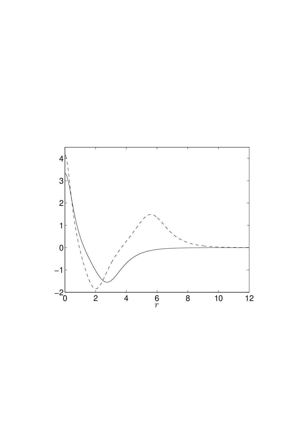
Refer to caption — Figure 1: Plot of $R_{1}$ (solid line) and $R_{2}$ (dashed line), normalized to unity, for $g_{0}=-0.5,\lambda=0.5$ . For these solutions $N_{1}\simeq 77.17$ and $N_{2}\simeq 195.84$ , respectively.

We have checked the “stationarity” of our numerically found solutions by propagating them through an homogeneous nonlinear medium subject to the perturbation coming from the numerical errors (both on the initial data and due to the roundoff error during the evolution). All our numerical simulations to be presented in this paper have been done using a second order in time and spectral in space split-step Fourier algorithm with absorbing boundary conditions to get rid of the outgoing radiation. In Fig. 2 we present the propagation of the norm and amplitude taking $u(x,y,0)=R_{1}(r)$ . As the stationary solutions of Eq. (3) are all unstable in the context of Eq. (1), one expects that sooner or later the instability will set in. In the case of the Townes and vortex solitons the instability sets in by $z\simeq 15$ and $z\simeq 3$ , respectively PRE. From the propagation of the norm and amplitude shown in Fig. 2, we can guess that, in our case, a collapse destroying the structure of this stationary state occurs near $z\simeq 11$ .

We have tried to apply the stabilization technique based on the modulation of the nonlinear coefficient to the first radially excited solution by setting $g(z)=g_{0}+g_{1}\cos(\Omega z)$ , with $g_{0}=-0.5$ , $g_{1}=-1.5$ and $\Omega=100$ (the parameters were set according to criteria established in Ref. Gaspar; IMACS) and taking $u(x,y,0)=R_{1}(r)$ . This mechanism allows a stable propagation of the Townes soliton over long distances of more than 400 units in adimensional units Gaspar but the same mechanism enhances only slightly the stability of singly-charged vortex solitons PRE. In principle our stationary solution has a simpler structure than the vortex and one could expect better results, but we will see that this is not true.

Our results are shown in Fig. 3. We can see how the inclusion of this periodic modulation leads to a shorter stable propagation distance of the structure and that collapse occurs by $z\simeq 6.5$

We have tried to stabilize this configuration by choosing different parameters for the modulation with similar results. We think that the reduction of the lifetime of the unstable stationary structure can be understood by considering the exchange of energy, i.e. energy flow, between the substructures of the first excited radially symmetric stationary solution: the central peak and its surrounding ring. During the defocusing ( $g(z)>0$ ) stages both substructures spread and overlap in the region where the field was zero previously. Then, in the focusing ( $g(z)<0$ ) stage the energy from the overlapping region flows mainly to the central peak. Therefore, with each focusing step the central peak is supplied with more and more energy, and this process leads finally to appearance of collapse (see the sharp amplitude peaks for $z\simeq 7$ in Fig. 3).

III Stabilization of higher-order radially symmetric solutions in vector layered media

III.1 Motivation and model

Our next idea is to try to stabilize the excited radially symmetric stationary solutionss by using a stabilized Townes soliton as a guide in which the higher order solution could be stabilized as it was done in Ref. PRE for vortices. Hence, we shift our attention to vector systems described by the following set of coupled NLS equations:


	$\displaystyle i\frac{\partial u_{1}}{\partial z}=-\frac{1}{2}\Delta u_{1}+g(z)\left(a_{11}\|u_{1}\|^{2}+a_{12}\|u_{2}\|^{2}\right)u_{1},$		(4a)
	$\displaystyle i\frac{\partial u_{2}}{\partial z}=-\frac{1}{2}\Delta u_{2}+g(z)\left(a_{21}\|u_{1}\|^{2}+a_{22}\|u_{2}\|^{2}\right)u_{2}.$		(4b)

Defining $\alpha=N(u_{2})/N(u_{1})$ and $\tilde{u}_{i}=u_{i}/N_{i}$ , $i=1,2$ Eqs. (4) become


$\displaystyle i\frac{\partial\tilde{u}_{1}}{\partial z}$	$\displaystyle=-\frac{1}{2}\Delta\tilde{u}_{1}+g(z)N_{1}\left(a_{11}\|\tilde{u}_{1}\|^{2}+\alpha a_{12}\|\tilde{u}_{2}\|^{2}\right)\tilde{u}_{1},$	(5a)
$\displaystyle i\frac{\partial\tilde{u}_{2}}{\partial z}$	$\displaystyle=-\frac{1}{2}\Delta\tilde{u}_{2}+g(z)N_{1}\left(a_{21}\|\tilde{u}_{1}\|^{2}+\alpha a_{22}\|\tilde{u}_{2}\|^{2}\right)\tilde{u}_{2},$	(5b)

For simplicity, we will discard the tilde in what follows and take both components to be normalized.

The parameter $\alpha$ is a measure of the strength of the interaction between both components, which could be accomplished experimentally by launching beams of different energies.

III.2 Case $\alpha=0$

In the limit $\alpha\rightarrow 0$ , corresponding to the case when the norm of one of the components is much smaller than the other, Eqs. (5) become


$\displaystyle i\frac{\partial u_{1}}{\partial z}$	$\displaystyle=$	$\displaystyle-\frac{1}{2}\Delta u_{1}+g(z)N_{1}a_{11}\|u_{1}\|^{2}u_{1},$	(6a)
$\displaystyle i\frac{\partial u_{2}}{\partial z}$	$\displaystyle=$	$\displaystyle\left[-\frac{1}{2}\Delta u_{2}+g(z)N_{1}a_{21}\|u_{1}\|^{2}\right]u_{2}.$	(6b)

Eq. (6a) is a scalar NLS equation with a modulated nonlinear coefficient and thus admits solutions in the form of stabilized Townes solitons. Eq. (6b) is a linear Schrödinger equation for $u_{2}$ in a trapping potential generated by $u_{1}$ . First we look for stationary solutions of Eqs. (6) when $g(z)=g_{0}$ of the form

	$\displaystyle u_{1}(\boldsymbol{r},z)$	$\displaystyle=$	$\displaystyle\phi_{\lambda}(r)\exp\left(-i\lambda z\right),$		(7)
	$\displaystyle u_{2}(\boldsymbol{r},z)$	$\displaystyle=$	$\displaystyle\varphi_{\mu}(r)\exp(-i\mu z),$		(8)

i.e. solutions of the nonlinear eigenvalue problem


$\displaystyle\lambda\phi$	$\displaystyle=$	$\displaystyle-\frac{1}{2}\Delta\phi+g_{0}N_{1}a_{11}\|\phi\|^{2}\phi,$	(9a)
$\displaystyle\mu\varphi$	$\displaystyle=$	$\displaystyle\left[-\frac{1}{2}\Delta\varphi+g_{0}N_{1}a_{21}\|\phi\|^{2}\right]\varphi.$	(9b)

Obviously, Eq. (6a) is equivalent to Eq. (3) and thus we get all of its stationary solutions, for instance, the Townes soliton. We will look for stationary solutions of Eq. (9b) with radial symmetry beyond the nodeless one $\varphi_{0}$ . This implies that the effective potential

V(r)=a_{21}g_{0}N_{1}|\phi_{\lambda}|^{2},

(10)

must support at least two bound states. The number of radially symmetric bound states supported by a two-dimensional potential is bounded by the inequality newton:

N_{2D,l=0}<1+\frac{1}{2}\frac{\int_{\mathbb{R}^{2}}dr\;dr^{\prime}\;rr^{\prime}\>V(r)\;V(r^{\prime})\;\left|\ln\left(\tfrac{r}{r^{\prime}}\right)\right|}{\int dr\>rV(r)}.

(11)

This inequality sets a necessary condition to have the required bound state (i.e. that with one node) for fixed $g_{0}=-2\pi$ by fixing a lower bound for the value of $a_{21}$ required to obtain $N_{2D,l=0}\geq 2$ . In Table 1 we show the lower bounds and the numerical results for the number of bound states obtained for several values of the coefficient $a_{21}$ . We can see that for $a_{12}=4$ we can have two modes in the effective potential generated by $R_{0}$ , the second one being a radially symmetric function with one node.

$a_{21}$	$N_{2D,l=0}$	Bound states eigenvalues
1	$<1.39$	$\lambda_{0}\simeq 0.575$
2	$<1.79$	$\lambda_{0}\simeq 1.925$
3	$<2.19$	$\lambda_{0}\simeq 3.558$
4	$<2.58$	$\lambda_{0}\simeq 5.335$ , $\lambda_{1}\simeq 0.195$

Table 1: Upper bound set by Eq. (11) on the number of bound states in two dimensions with radial symmetry and without angular momentum of the potential

V(r)=a_{21}g_{0}N_{1}|R_{0}|^{2}

\lambda_{0}

and

\lambda_{1}

are the approximate eigenvalues of the ground and first excited states of

V(r)

, respectively, found numerically.

We have computed the profile of the radially symmetric solution of Eq. (6b) with one node in $\varphi_{1}$ which exists for $a_{21}=4$ by using a standard shooting method, which is shown in Fig. 4

We have propagated numerically the initial data $u_{2}=\varphi_{1}$ according to Eq. (6b) alone but now with a periodically varying nonlinear coefficient. During the propagation the potential $a_{21}g(z)|R_{0}|^{2}$ oscillates with frequency $\Omega$ due to the periodic modulation of coefficient $g(z)$ , hence, the potential will change its behavior periodically from attractive to repulsive. In general, for the linear situation described by Eq. (6b), one may achieve a non-dispersive propagation for small oscillations of $g(z)$ , i.e. without being necessary to change its sign. However, as we are interested to extend these results to the full nonlinear equations, we must construct $g(z)$ with an alternating sign because analytical results Konotop; Gaspar and computer simulations Gaspar have revealed that this is a requirement to get stabilized solitons.

Using results from the quantum mechanical theory of fast perturbations galindo we have chosen a set of parameters, $g_{0}=-2\pi$ , $g_{1}=8\pi$ and $\Omega=100$ for which the oscillating behavior of $g(z)$ should maintain the profile of the excited solution in $u_{2}$ . Moreover, this set of parameters leads to an stabilized Townes soliton in component $u_{1}$ IMACS. In Fig. 5 we can see that although the maximum value of the amplitude exhibits oscillations related to the periodic modulation of $g(z)$ , the norm remains constant which indicates that no radiation is emitted while the potential $a_{21}g(z)|u_{1}|^{2}$ is switched from attractive to repulsive.

Next we take $u_{1}=R_{0},u_{2}=U_{1}$ as initial data for Eqs. (6). This situation is described by the case of $\alpha\simeq 0$ , which means that the energy injected into the medium by the second component $u_{2}$ is much smaller in comparison with that of the first component $u_{1}$ PRE. The dynamics of the most important parameters of the system is plotted in Figure 6.

We want to remark that the time evolution of $|u_{1}|^{2}$ exhibits high and low frequency oscillations corresponding to the periodic modulation of $g(z)$ and to the internal dynamics of Eq. 6a, respectively Gaspar. Therefore, the potential experienced by $u_{2}$ includes this oscillation pattern. As the low frequency oscillations do not fulfill the requirements PRE derived from the theory of fast perturbations, they lead to energy emission from the second component $u_{2}$ . The radiation emission is linked to the decreasing value of the $u_{2}$ norm: as the outgoing radiation hits the boundary of the computational domain it is removed by an absorbing potential. Nevertheless, the first component evolves unperturbed as a stabilized Townes soliton Gaspar.

The spatial intensity profile of the propagating beam $u_{2}$ , see Fig. 7, has similar shape to the initial one (see Fig. 1). However, the maximum of the intensity distribution in Fig. 6(b) is about three times smaller than the corresponding value of the initial one due to the energy loss during the propagation.

III.3 Weak nonlinear coupling

Finally we turn on the nonlinear coupling in system (5) by setting $\alpha=0.1$ . The dynamics of the system parameters is presented in Figure 8.

One can see that the propagation of the excited state is drastically changed in comparison with the previous analyzed cases. Under the effect of the nonlinear coupling, both components $u_{1}$ and $u_{2}$ reshape their transverse spatial profile by emitting energy. After a short propagation distance, $z=25$ , the excited solution losses its spatial shape, acquiring a profile which resembles to the Townes soliton and which will be propagate along with the Townes soliton. We may say that both initial profiles decay or readjust (with energy loss) their shape, eventually leading to the formation of nodeless stabilized vector solitons PROLO. Nevertheless, for smaller values of $\alpha$ , e.g. $\alpha=0.05$ , we recover the behaviour described in the previous subsection, with shape preservation accompanied by energy emission.

We think that the mechanism described at the end of Section II is responsable for the decay of component $u_{2}$ when the nonlinear coupling is large enough. The changes taking place in the component $u_{2}$ are then coupled back to component $u_{1}$ , which leads to energy emission, as seen by the decreasing norm of $u_{1}$ in Figure 8.

IV Solutions without radial symmetry

Equation (3) has more solutions beyond those having radial symmetry. For instance, Alfimov and coworkers Alfimov, using branching-off techniques from the theory of dynamical systems constructed solutions having nontrivial discrete rotational symmetries. Two examples of those solutions are shown in Fig. 10. In all of them we observe that a large central peak is surrounded by smaller ones having the prescribed discrete symmetry plus an outer ring.

Since these solutions are also unstable, their free propagation leads to collapse as shown in Figs. 11 and 12. Since their norms are much above the critical one both solutions suffer a fast instability to collapse, the constant behavior of the norm indicating the fact that outgoing radiation waves have no time to escape from this system before the instability develops. The sensitivity of those configurations to collapse manifests itself in the fact that the instability distances are two orders of magnitude smaller than those of simpler solutions such as the Townes, vortex or first radially excited solitons.

We have tried to use the modulation of the nonlinear coefficient to stabilize the stationary solutions presented in Fig. 10. However, the time evolution of the beam parameters does not change appreciably and in particular, the emergence of collapse cannot be delayed. We have tried unsucessfully different sets of parameters to achieve stabilization. Intuitively, it seems difficult to be able to stabilize those complicated structures because of the coexistence of different types of substructures (peaks, rings, etc) and the fact that their norm ar many times the critical one (see the caption of Fig. 10).

V Conclusions

In this paper we have complemented previous knowledge on stabilized solitons of the Nonlinear Schrödinger Equation by studying numerically the possibility of stabilizing excited stationary solutions with radial symmetry in both (i) scalar and (ii) vectorial layered media. The scalar system is unable to stabilize radially excited states due to the internal dynamics, i.e. energy flow, of this state which leads to shorter stable propagation distances of the beam and collapse when compared with the propagation of the same beam through homogeneous media. In the case of vector layered media we have shown how weakly coupled beams when one of the components is chosen to be the Townes soliton and the other an unstable radially excited solution can be stabilized. In this situation it is found that the radially excited state radiates continuously energy while preserving an intensity shape similar to the initial profile.

In both scalar and vectorial layered media, the stabilization of solutions bearing nontrivial structure is difficult to achieve. This fact is due to the ireversibility of the internal energy flows between the wave substructures, e.g. rings, peaks, during propagation. Additional stabilizing mechanisms, like spatially inhomogeneous nonlinearities depending on the transverse variables, might help in stabilizing states with nontrivial structures as it happens in the case of non-oscillating structures U1; U2; U3.

Finally, we have tried unsuccesfully to stabilize complex asymmetric solutions of Eq. (1). The complex structure of these solutions and the fact that their power is many times the critical power makes stabilization probably impossible.

Acknowledgements.

We want to thank G. Alfimov for discussions. This work has been partially supported by grants FIS2006-04190 (Ministerio de Educación y Ciencia, Spain) and PAI-05-001 (Consejería de Educación y Ciencia de la Junta de Comunidades de Castilla-La Mancha, Spain),

References

(1) C. Sulem, P. Sulem, The Nonlinear Schrödinger Equation: Self-focusing and Wave Collapse, Springer, Berlin, 2000.
(2) L. Vázquez, L. Streit, and V. M. Pérez-García, Eds., Nonlinear Klein-Gordon and Schrödinger systems: Theory and Applications, World Scientific, Singapur (1997).
(3) F. Brezzi, and P. A. Markowich, Math. Mod. Meth. Appl. Sci. 14 (1991) 35; J. L. López, J. Soler, Math. Mod. Meth. in App. Sci., 10 (2000), 923-943.
(4) Y. Kivshar, and G. P. Agrawal, Optical Solitons: From fibers to Photonic crystals, Academic Press (2003).
(5) A. Hasegawa, Optical Solitons in Fibers, Springer-Verlag, Berlin, (1989).
(6) R.K. Dodd, J.C. Eilbeck, J.D. Gibbon, and H.C. Morris, Solitons and nonlinear wave equations, Academic Press, New York (1982).
(7) J. L . Rosales, J. L. Sánchez-Gómez, Phys. Lett. A 66 111 (1992).
(8) R. Fedele, G. Miele, L. Palumbo, and V. G. Vaccaro, Phys. Lett. A 173 407 (1993).
(9) F. Dalfovo, S. Giorgini, L. P. Pitaevskii, and S. Stringari, Rev. Mod. Phys. 71 463 (1999).
(10) A.S. Davydov, Solitons in Molecular Systems, Reidel, Dordrecht (1985).
(11) L. Berge, V.K. Mezentsev, J.J. Rasmussen, P.L. Christiansen, Y.B. Gaididei, Opt. Lett. 25, 1037 (2000).
(12) I. Towers and B. A. Malomed, J. Opt. Soc. Am. B 19, 537 (2002).
(13) H. Saito and M. Ueda, Phys. Rev. Lett. 90, 040403 (2003).
(14) F. Abdullaev, J. G. Caputo, R. Kraenkel, and B. A. Malomed, Phys. Rev. A 67, 013605 (2003).
(15) G. D. Montesinos, V. M. Pérez-García and P. Torres, Physica D (Amsterdam) 191, 193 (2004).
(16) G. D. Montesinos, V. M. Pérez-García, Math. Comp. Simul. 69, 447-456 (2005).
(17) V. V. Konotop, P. Pacciani, Phys. Rev. Lett. 94, 240405 (2005).
(18) M. Centurion, M. A. Porter, P. G. Kevrekidis, and D. Psaltis, Phys. Rev. Lett. 97, 033903 (2006).
(19) M. Centurion, M. A. Porter, Y. Pu, P. G. Kevrekidis, D. J. Frantzeskakis, and D. Psaltis, Phys. Rev. Lett. 97, 234101 (2006).
(20) S. K. Adhikari, Phys. Rev. A 69, 063613 (2004).
(21) H. Saito, M. Ueda, Phys. Rev. A 70, 053610 (2004).
(22) G. D. Montesinos, V. M. Pérez-García, H. Michinel, Phys. Rev. Lett. 92 133901 (2004).
(23) G. D. Montesinos, M. I. Rodas-Verde, V. M. Pérez-García, H. Michinel, Chaos 15, 033501 (2005).
(24) F. Abdullaev, J. Garnier, Phys. Rev. E 72, 035603 (2005).
(25) V. Zharnitsky and D. Pelinovsky, Chaos 15, 37105 (2005).
(26) S. Cuccagna, E. Kirr, and D. Pelinovsky, J. Diff. Eqs. 220, 85 (2006).
(27) V. M. Pérez-García, V. V. Konotop, P. Torres, Physica D 221, 31 (2006).
(28) A. Itin, S. Watanabe, T. Morishita, Phys. Rev. A 74, 033613 (2006).
(29) F. K. Abdullaev, A. Gammal, A. Kamchatnov, L. Tomio, Int. Jour. of Mod. Phys. B, 19 (2005) 3415.
(30) B. A. Malomed, Soliton Management in Periodic Systems, Springer-Verlag (Berlin, 2006).
(31) G. D. Montesinos, V. M. Pérez-García, H. Michinel, J. R. Salgueiro, Phys. Rev. E 71, 036624 (2005).
(32) G. L. Alfimov, V. M. Eleonski, N. E. Kulagin, L. M. Lehrmann and V. P. Silin, Phys. Lett. A 138, 443-446 (1989).
(33) R. Y. Chiao, E. Garmire, and C.H. Townes, Phys. Rev. Lett. 13, 479 (1964).
(34) R. G. Newton, J. Math. Phys. 3, 867 (1962).
(35) A. Galindo and P. Pascual, Quantum Mechanics I & II, (Springer Verlag, Berlin, 1990).
(36) G. Fibich, and X.-P. Wang, Physica D 175, 96-108 (2003).
(37) H. Sakaguchi and B. Malomed, Phys. Rev. E, 73, 026601 (2006).
(38) G. Dong, B. Hu, and W. Lu, Phys. Rev. A 74, 063601 (2006).