Lyapunov Modes for a Nonequilibrium System with a Heat Flux
Abstract
We present the first numerical observation of Lyapunov modes (mode structure of Lyapunov vectors) in a system maintained in a nonequilibrium steady state. The modes show some similarities and some differences when compared with the results for equilibrium systems. The breaking of energy conservation removes a zero exponent and introduces a new mode. The transverse modes are only weakly altered but there are systematic changes to the longitudinal and momentum dependent modes.
1 Introduction
The difference of two trajectories starting from infinitesimally nearby initial conditions, which is called the Lyapunov vector, plays an essential role in the description of stability or instability in dynamical systems. The exponential rate of expansion or contraction of the absolute value of the Lyapunov vector is the Lyapunov exponent, and its positivity means that the system has a dynamical instability and is called chaotic. The Lyapunov vector is introduced in each independent direction of phase space, so in general we have to consider a set of Lyapunov exponents, called the Lyapunov spectrum, and the corresponding Lyapunov vectors in a high-dimensional chaotic system. An algorithm to calculate the Lyapunov exponents and vectors in many-body systems has been developed by Benettin et al. [1, 2, 3], and Shimada and Nagashima [4], and the behavior of Lyapunov vectors has been investigated from various points of view, for example, the conjugate pairing rule for Lyapunov spectra in some thermodynamic systems [5, 6, 7, 8], and the localization behavior of Lyapunov vectors [9, 10, 11, 12, 13, 14, 15, 16], etc.
Recently, wavelike structure of Lyapunov vectors, called Lyapunov modes, and the corresponding stepwise structure of Lyapunov spectra has drawn attention in many-particle chaotic systems [17, 18, 19, 20, 21, 22, 23]. This structure appears in the region of Lyapunov exponents with small absolute values. Lyapunov exponents have the dimension of inverse time, so the structure in the small Lyapunov exponents is supposed to be a reflection of the slow and macroscopic behavior of many-particle systems. Since the first observation of Lyapunov modes in computer simulations of hard disk systems [18, 24, 25, 26, 27] they have been found in systems with soft potentials, independent of dimensionality and system geometry. It is now believed that the zero modes arise due to the presence of conserved quantities [28], and the spatial dependence of the non-zero modes is essentially analogous to higher order Fourier components. It has been shown that the breaking of conserved quantities, by for example a change from periodic to hard wall boundary conditions, leads to the absence of particular modes. It is also known that there are stationary modes and time-oscillating modes among the non-zero Lyapunov modes, and the time-oscillating period of the Lyapunov modes is connected to that of an equilibrium momentum auto-correlation function [26, 28].
In this paper we consider the effect of breaking energy conservation by adding energy at one end of the system and removing it at the other. Although this leads to a flow of heat energy through the system, this is not intended to be a realistic model of low dimensional heat flow. Quasi-one-dimensional systems have been extensively used to investigate Lyapunov modes and the localization or delocalization of Lyapunov vectors for many-particle systems at equilibrium [25, 26, 15, 16], and these systems can easily be adapted to maintain a heat flow. Using such a system, we investigate nonequilibrium effects of the Lyapunov modes and the momentum auto-correlation functions.
2 Quasi-One-Dimensional Heat Model
We consider a quasi-one-dimensional many-hard-disk system with a mechanism to insert energy at one end of the system and to remove energy from the other end. It consists of hard disks of radius and mass in a two-dimensional rectangular region of length and width , with so that the disk order remains invariant. We choose periodic boundary conditions in the transverse -direction, and in the longitudinal -direction we use a special boundary condition that allows the transfer of energy between the system and walls:
| (1) | |||||
| (2) |
where , is Boltzmann’s constant and is a parameter (). In a collision, is the incoming momentum of the particle and is the outgoing momentum. The parameter controls the strength of the coupling to the “heat reservoir” of temperature (where is either or ). When the incoming momentum is completely replaced by the mean thermal momentum of the reservoir and all information contained in the incoming momentum is lost. At the connection with the reservoir is removed and the collision process is hard wall. Here we consider values of between and so that the reservoir is coupled to the system but the loss of information is not complete. We choose the temperatures of the reservoirs independently, so the temperature of the left-hand side reservoir is , and the right-hand side reservoir is . A schematic illustration of this system is given in Fig. 1. For the numerical results that are shown in this paper, we use the values , , , and .

Note that boundary condition (2) with periodic boundary conditions in the -direction guarantees that the total momentum in the -direction is conserved. The parameter determines the strength of the coupling between the reservoir and the system, and specifies the fraction of incoming momentum that is retained after the collision. If and then an energy transfer (heat) occurs across the system, and a nonequilibrium steady state is established after a long time.
3 Stepwise Structure of Lyapunov Spectra

Figure 2 is a graph of the absolute value of the normalized Lyapunov spectrum with . Here the largest Lyapunov exponent is . From this figure we see that the positive branch and the negative branch of the Lyapunov spectrum are not symmetric, namely particularly for the exponents of smallest magnitude near . This is different from the equilibrium case () where the dynamics is Hamiltonian with the symplectic structure guaranteeing the conjugate pairing rule for the Lyapunov spectra [29]. The system has 3 zero-Lyapunov exponents, due to total momentum conservation and spatial translational invariance in the direction, and time-translational invariance. In the nonequilibrium case () the total energy of the system is no longer conserved and this is the reason that , although it is zero at equilibrium.
| Positive | branch | Negative | branch | |
|---|---|---|---|---|
| Step number | 1-point step | 2-point step | 1-point step | 2-point step |
| First | 198 | 197, 196 | 203 | 204, 205 |
| Second | 195 | 194, 193 | 206 | 207, 208 |
| Third | 192 | 191, 190 | 209 | 210, 211 |
In Refs. [25, 26, 28], it is shown that for the equivalent equilibrium system (that is, and hard-wall boundary conditions in the longitudinal direction and periodic boundary conditions in the transverse direction), the Lyapunov spectrum consists of 1-point steps and 2-point steps. The 1-point steps correspond to Lyapunov vectors containing transverse Lyapunov modes, and have their origin in total momentum conservation (and translational invariance) in the direction. On the other hand, the 2-point steps correspond to longitudinal and momentum proportional mode contributions. In Fig. 2 we can see that, away from equilibrium, the 1-point steps and 2-point steps remain (see Table 1 for meaning of 1-point and 2-point steps of the Lyapunov spectrum). The positive and negative branch 1-point steps are symmetric, that is , for . This may be because total momentum conservation and spatial translational invariance in the direction is preserved regardless of the value of . On the other hand, the step-heights of the 2-point steps are clearly different in the positive and negative branches. Indeed, the asymmetry of the positive and negative exponents appears to be of the same magnitude for each 2-point step, and as well as for exponent that has shifted from zero.
There is no Gaussian thermostat [6, 7] in this system so conjugate pairing of Lyapunov exponents would not be expected to hold. The magnitudes of the largest and smallest Lyapunov exponents appear to be almost equal, and there is only weak evidence for phase space dimensional contraction because dissipation as the origin of such a contraction can occur only at the two particles at the ends of the system.
4 Mode Structure of Lyapunov Vectors
For each Lyapunov exponent in the Lyapunov spectrum there is a corresponding Lyapunov vector which will in general have both coordinate and momentum components. For the exponents of smallest magnitude, the Lyapunov vectors often contain either coordinates of momentum components that vary sinusoidally with particle position forming a delocalized structure. We refer to such Lyapunov vectors containing delocalized structures as Lyapunov modes.
4.1 Modification of zero-Lyapunov Modes
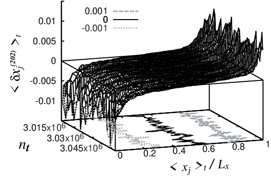
The introduction of the nonequilibrium boundary condition leads to a change in the structure of the Lyapunov mode corresponding to exponent . The component of the new mode is shown in Fig. 3. The fact that , is a purely nonequilibrium effect. Figure 3 shows the longitudinal component of the Lyapunov vector as a function of the collision number and the normalized particle position for . Note that in this paper the Lyapunov vector corresponding to the Lyapunov exponent is normalized so that . In order to obtain a clear graph, we take a local time average, indicated by the notation , over collisions using data just after collisions. Figure 3 shows an approximately steady structure with a slope which is steepest near the two ends of the system. This structure is quite different from the equilibrium case, where the longitudinal component is found numerically to be almost zero in both space and time.
4.2 Transverse Lyapunov Modes

Each 1-point step of the Lyapunov spectrum has an associated Lyapunov vector containing a transverse mode. The component for the -th disk of the Lyapunov vector has a sinusoidal dependence on the particle position at equilibrium [25, 26]. We show that this structure is only slightly changed when the system is driven away from equilibrium, . In Fig. 4 we present the time average of the transverse mode as functions of the average position of the -th disk for different values of . The first (), second () and third () transverse modes are clearly visible for the nonequilibrium cases. Note that the transverse Lyapunov modes in Fig. 4 show a weak -dependence. In the nonequilibrium case , there is a deviation from a sinusoidal curve in the transverse mode, while in the equilibrium case , the mode structure can be fitted nicely by a sinusoidal curve. Fig. 4 shows that the amplitude of the transverse mode decreases slightly from the high temperature region (left side) to the low temperature region (right side). This change in amplitude in the transverse Lyapunov modes is a nonequilibrium effect .
4.3 Longitudinal and Momentum-Proportional Lyapunov Modes

Some of the structure of the longitudinal modes in the system remains as the system departs from equilibrium. There is a phase shift in time between the components of modes in the same 2-point step, that is between and , see Fig. 5. As the momentum components are approximately the same functional form as the spatial components, there is the same phase shift between and . The same behavior is observed for the components of the modes in the first 2-point step in the negative branch of the spectrum, and differ by a phase shift in time, as do the contributions and . In the positive branch 2-point step the spatial contributions are larger than the momentum contributions, in the negative branch the relative sizes of the contributions are reversed.
The principle new feature is that nodal lines are curved, with those contributions to the positive branch of the spectrum having the center of the system reaching the node later than the two ends. This gives the appearance of a “forward” moving wave in the positive branch modes and a “backward” moving wave in the negative branch modes. It is less apparent in Fig. 5 that the time-oscillating period in the negative branch is larger than that for the positive branch. Also, the components in the negative branch do not have nodes at the two ends but these are shifted within the boundaries.

The momentum proportional components of the modes in Fig. 6 are also similar to those at equilibrium. The phase differences of and the straight nodal lines remain the same. However, the central nodal line at is now shifted towards the high temperature end of the system for both and . As with the longitudinal modes, the time-oscillating period in the negative branch is larger than in the positive branch. The other modes that are not shown in Fig. 6 have a similar structure, for example for and have a similar structure to but with more apparent noise. Also, for and have a similar structure to but with more apparent noise.
5 Time-Oscillating Periods of Lyapunov modes and Velocity Auto-Correlation

| 0 | 0.5 | 0.9 | |
|---|---|---|---|
| 8210 | 8560 | 8830 | |
| 5700 | 5700 | 5600 | |
| 8300 | 8200 | 8100 | |
| 16400 | 16200 | 14900 | |
| 16400 | 19600 | 56400 | |
| 8300 | 9300 | 12500 | |
| 5700 | 6300 | 8100 |
The period (in numbers of collisions) of the auto-correlation function (acf) for the longitudinal component of the momentum increases, and the amplitude decreases as a function of (see Table 2). The time oscillating period of the Lyapunov vectors for the -th longitudinal (and the momentum proportional) mode in the positive branch of the Lyapunov spectrum decreases slightly as a function of , whereas in the negative branch the period increases slightly as a function of . Such changes of are especially large for small ’s, which correspond to the ones close to the zero-Lyapunov exponents. The relation is not correct away from equilibrium, while it is justified in equilibrium [26, 28]. This does not contradict the proof of this relation as that required equilibrium and is based on the functional form of the Lyapunov modes, in particular that they are purely sinusoidal.
6 Conclusion and Remarks
The changes in the structure of the Lyapunov modes for a system maintained away from equilibrium by a boundary imposed heat flow are described in detail. The breaking of conservation of energy is shown to introduce systematic effects, changing the number of zero exponents, and modifying the form of other modes, with the basic structure of transverse, longitudinal and momentum proportional modes remaining. This work is largely descriptive and the theoretical origin of the changes in modes is yet to be developed, as it is for the equilibrium case. However, it is clear that the modes are not only equilibrium properties of many-particle systems, but also fundamental for nonequilibrium steady states.
The original purpose in introducing the nonequilibrium boundary conditions [i.e. Eqs. (1) and (2)] was to keep dynamical properties, like the momentum conservation in the transverse direction and deterministic property of orbit, etc., in a nonequilibrium dynamics while breaking energy conservation. The equilibrium case is recovered in the limit as . Therefore this choice of the boundary conditions was not intended to provide a realistic model for the interaction between a heat reservoir and a particle system. For example, a consequence of these boundary conditions is that the momentum distribution function for a particle in contact with the reservoir is very different from a Gaussian. Indeed, we found that the incoming momentum is close to Gaussian but the outgoing momentum is strongly peaked around the mean momentum of the reservoir, with the width of its distribution determined by the degree of mixing with the incoming momentum (that is, determined by the value of ).
Acknowledgement
The authors appreciate a careful reading of the manuscript by E. G. D. Cohen, and the financial support of the Japan Society for the Promotion of Science.
References
- [1] G. Benettin, L. Galgani, and J. -M. Strelcyn, Phys. Rev. A 14, 2338 (1976).
- [2] G. Benettin, L. Galgani, A. Giorgilli, and J. -M. Strelcyn, Meccanica 15, 9 (1980).
- [3] G. Benettin, L. Galgani, A. Giorgilli, and J. -M. Strelcyn, Meccanica 15, 21 (1980).
- [4] I. Shimada and T. Nagashima, Prog. Theor. Phys. 61, 1605 (1979).
- [5] U. Dressler, Phys. Rev. A 38, 2103 (1988).
- [6] D. J. Evans, E. G. D. Cohen, and G. P. Morriss, Phys. Rev. A 42, 5990 (1990).
- [7] C. P. Dettmann and G. P. Morriss, Phys. Rev. E 53, R5545 (1996).
- [8] T. Taniguchi and G. P. Morriss, Phys. Rev. E 66, 066203 (2002).
- [9] P. Manneville, Lecture Note in Physics, 230, 319 (1985).
- [10] K. Kaneko, Physica D 23, 436 (1986).
- [11] R. Livi and S. Ruffo, in Nonlinear Dynamics, edited by G. Turchetti (World Scientific, Singapore, 1989), p. 220.
- [12] M. Falcioni, U. M. B. Marconi, and A. Vulpiani, Phys. Rev. A 44, 2263 (1991).
- [13] G. Giacomelli and A. Politi, Europhys. Lett. 15, 387 (1991).
- [14] Lj. Milanović and H. A. Posch, J. Mol. Liquids, 96-97, 221 (2002).
- [15] T. Taniguchi and G. P. Morriss, Phys. Rev. E 68, 046203 (2003).
- [16] T. Taniguchi and G. P. Morriss, Phys. Rev. E 73, 036208 (2006).
- [17] Ch. Dellago, H. A. Posch, and W. G. Hoover, Phys. Rev. E 53, 1485 (1996).
- [18] H. A. Posch and R. Hirschl, in Hard ball systems and the Lorentz gas, edited by D. Szász (Springer, Berlin, 2000), p. 279.
- [19] J. -P. Eckmann and O. Gat, J. Stat. Phys. 98, 775 (2000).
- [20] T. Taniguchi and G. P. Morriss, Phys. Rev. E 65, 056202 (2002).
- [21] S. McNamara and M. Mareschal, Phys. Rev. E 64, 051103 (2001).
- [22] A. S. de Wijn and H. van Beijeren, Phys. Rev. E 70, 016207 (2004).
- [23] T. Taniguchi, C. P. Dettmann, and G. P. Morriss, J. Stat. Phys. 109, 747 (2002).
- [24] H. L. Yang and G. Radons, Phys. Rev. E 71, 036211 (2005).
- [25] T. Taniguchi and G. P. Morriss, Phys. Rev. E 68, 026218 (2003).
- [26] T. Taniguchi and G. P. Morriss, Phys. Rev. E 71, 016218 (2005).
- [27] J. -P. Eckmann, C. Forster, H. A. Posch, and E. Zabey, J. Stat. Phys. 118, 813 (2005).
- [28] T. Taniguchi and G. P. Morriss, Phys. Rev. Lett. 94, 154101 (2005).
- [29] V.I. Arnold, Mathematical Methods of Classical Mechanics, 2nd ed. Springer-Verlag, Berlin, 1989.