Intermediate wave-function statistics
Abstract
We calculate statistical properties of the eigenfunctions of two quantum systems that exhibit intermediate spectral statistics: star graphs and Šeba billiards. First, we show that these eigenfunctions are not quantum ergodic, and calculate the corresponding limit distribution. Second, we find that they can be strongly scarred, in the case of star graphs by short (unstable) periodic orbits and in the case of Šeba billiards by certain families of orbits. We construct sequences of states which have such a limit. Our results are illustrated by numerical computations.
pacs
Valid PACS appear hereIt has been conjectured that the quantum spectral statistics of systems that are chaotic in the semi-classical limit are generically those of Random Matrix Theory Bohigas et al. 1984. The behaviour of the eigenfunctions of such systems is described by the semi-classical eigenfunction hypothesis Berry 1977a; Voros 1979, which implies that they equidistribute over the appropriate energy shell. This is in agreement with a theorem of Schnirelman Schnirelman 1974 which implies equidistribution of almost all eigenstates on scales independent of , assuming only classical ergodicity. Such behaviour is termed quantum ergodicity. This theorem still permits the possibility of a small number of states which do not equidistribute.
It has been suggested that some of these exceptional states may be “scarred” by short classical periodic orbits Heller 1984. Further investigations Bogomolny 1988; Berry 1989; Keating and Prado 2001; Agam and Fishman 1994; Kaplan 1999; Schanz and Kottos have distinguished between weak and strong scarring. Weak scarring relates to states averaged over energy windows that contain a semi-classically increasing number of levels, whereas strong scarring means that sequences of states can be constructed whose limit is wholly or in part supported by one-or-more periodic orbits. So far the only systems known rigorously to support strong scarring are the cat maps Faure et al., which have non-generic spectral statistics Keating 1991.
For systems that are classically integrable, it is expected that the quantum spectral statistics are Poissonian, i.e. those of independent random numbers Berry and Tabor 1977. The corresponding eigenfunctions semiclassically equidistribute on tori in phase space Berry 1977b.
Recently, classes of systems which exhibit spectral statistics that are intermediate between Random Matrix and Poissonian have been discovered Shklovskii et al. 1993; Bogomolny et al. 2001a; Bogomolny et al. 2001b. Two representative families of examples are Šeba billiards Šeba 1990 and star graphs Berkolaiko and Keating 1999. It was shown in Berkolaiko et al. 2001 that these two systems have the same (intermediate) spectral statistics. We study the eigenfunction statistics of such systems. Specifically, given that these systems are not classically ergodic, we are interested in whether the eigenfunctions are quantum ergodic, and whether they show strong scarring (that they exhibit weak scarring may be shown using the methods of Bogomolny 1988).
Star graphs are quantum graphs Kottos and Smilansky 1999 which have one central vertex, and outlying vertices each connected only to the central vertex Berkolaiko and Keating 1999. For such graphs, the limit is analogous to the semi-classical limit. To investigate the possibility of quantum ergodicity in this limit, we consider a graph with bonds, where , , and introduce the observable defined by
Thus picks out a fraction of the bonds. Let denote the wave-function associated with the eigenstate. We calculate the probability distribution, , for chosen at random, that is less than , subject to some mild restrictions on the bond lengths. A system which exhibits quantum ergodicity would have
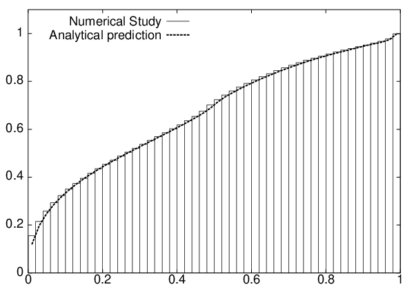
Our result (see equation (8) and figure 1 below) differs from this, proving that star graphs are not quantum ergodic. In fact we are able to say more: for a fixed (finite) number of bonds, we explicitly find eigenstates that are strongly scarred along closed (unstable) orbits of the graph with period 2. This is the first class of examples showing generic (in this case intermediate) behaviour in which strong scarring has been rigorously demonstrated.
The term Šeba billiard refers to any integrable quantum system that has been perturbed by the addition of a point singularity. We consider the specific example of a billiard on a torus. By exploiting the connection between Šeba billiards and star graphs Berkolaiko et al. 2001 we argue that Šeba billiards are also not quantum ergodic and find states that appear to show behaviour analogous to strong scarring, in this case by families of orbits.
We begin by describing how to calculate the probability distribution .
Eigenenergies of a star graph with bonds are given by , where is the solution of with
| (1) |
the individual bond lengths being denoted by . The component of the wave-function on the bond of the graph is , where
| (2) |
the sum being taken over all bonds. Then
| (3) |
To calculate the distribution of values taken by this quantity we average over a large number of states, making the error term in (3) negligible. We choose incommensurate bond lengths from an interval that shrinks in such a way that as . Thus we can replace by wherever it does not multiply .
To evaluate a function at the zeros of we integrate against the density of states, so
where denotes the Dirac delta function. Writing the delta function in Fourier representation, , and taking the limit ,
| (4) | |||||
writing and using , where is the mean density of states. We apply (4) with where
| (5) |
for constants. This is related to the distribution of by the fact that
when and are related by .
We observe that only appears in (4) multiplied by a bond length, and as an argument of a -periodic function. Since the bond lengths are incommensurate, the integral can be re-written as a multiple integral over the variables . A similar argument was used in Barra and Gaspard 2000; Keating et al.. The integrand then factorises, so that
| (6) | |||||
where
is obtained by replacing with in , and by making the same substitution in . Techniques to analyse the asymptotics of these integrals were discussed in Keating et al.. Using them we find that
and
as . Substituting the above into (6) and denoting the result , we arrive at
where
and
The Fourier transform of is the probability density function of where the index of the state, , is chosen at random. The probability distribution for to be less than is then given by
| (7) |
The Fourier transform of is
having made the substitution and using the notation . Performing the -integral in (7) gives, finally,
| (8) |
with , for .
We now turn to constructing sequences of eigenstates on star graphs, when is fixed, that are strongly scarred by certain short periodic orbits. (Note that on such graphs all orbits are unstable.) Our construction exploits the properties of the spectral determinant (1). The spectral determinant has poles at the points
Since the derivative of is everywhere greater than zero, there is exactly one root of between every two consecutive poles.
Given a small , which will control the quality of the scarred eigenstate, we can find a pole in the set satisfying the following properties: (a) there is a pole from within a distance of and (b) is approximately equidistant from the two nearest poles from , for each . Due to the ergodic properties of the sequence (assuming that the bond lengths are incommensurate), the above situation occurs with non-zero frequency along the -axis.
Denote the root squeezed between and by . Then is of the order of when and is of order otherwise. Going back to the eigenstate formula (2), we see that
that is, the amplitude of the -eigenstate on the bonds 1 and 2 is times stronger than on any other bond. By selecting suitably small one can find eigenstates localized on any two given bonds to any precision. Understandably, higher precision leads to a smaller frequency of the scarred eigenstates. In fact, the frequency is proportional to .
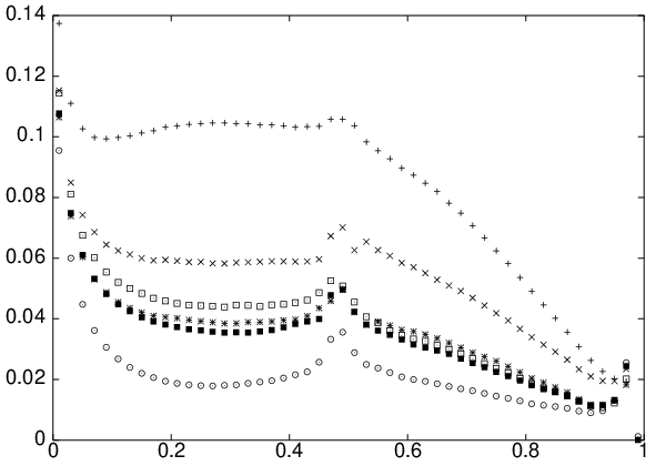
Since it follows that which provides an explanation for the visible singularity at in the difference between for finite and its limiting form (see figure 2). This singularity corresponds to the eigenstates localized on bonds and such that is picked out by the observable and is not.
The above construction can be generalized to produce eigenstates localised on any number of bonds. However, once , the amplitudes on the bonds are generally not equal, which explains the lack of singularities at rational fractions other than . Finally, the singularities at and correspond to the cases when the eigenstates are localized fully outside () or inside () the bonds picked out by .
The preceding calculations can be made rigorous. We defer the details to Berkolaiko et al..
In Keating et al. it was suggested that the squares of the coefficients, , of the eigenfunctions of Šeba billiards expressed in the basis of states of the unperturbed billiard
| (9) |
are distributed in the same way as the square of the maximum norm on a single bond of a star graph in the limit as . This conjecture was supported by numerical evidence. We extend this analogy to interpret the above results in terms of the Šeba billiard. Since the quantity in (3) is similar to a sum of norms of eigenfunctions on a fraction of bonds, we conjecture that the sum of the squares of a fraction of the coefficients has probability distribution . To elucidate this idea, consider preparing a Šeba-type system in a randomly-chosen eigenstate. The perturbation is then removed instantaneously, and a measurement of the energy is made. What is the distribution (with respect to the choice of initial state) of the probability that the measured energy is one of a given fraction of the energy levels of the unperturbed system? The answer is the distribution function in (8). If the eigenfunctions of the billiard were asymptotically equidistributed then this probability distribution would be a unit step function at .
Energy levels of a Šeba billiard interlace with energy levels of the original unperturbed system in much the same way that momenta of star graphs interlace with poles of the function . We consider a Neumann billiard in a rectangle with aspect ratio , perturbed by a point singularity at the origin. Eigenstates of this system can be expanded as
| (10) |
where is a normalisation constant, the energy levels of the Neumann billiard are , and are the corresponding eigenfunctions. It is well known that these unperturbed eigenfunctions are localised in momentum space. We therefore expect to find states of the Šeba billiard that exhibit structures analogous to scars in momentum space when their energy is between two closely spaced levels of the unperturbed billiard. In fact such states will scar in two directions in momentum space, corresponding to the two unperturbed eigenstates closest in energy to the state in question. These scars are supported by families of orbits corresponding to tori in the unperturbed system. Note however that torus quantisation itself does not apply. It is in this sense that the structures are analogous to scars.
Figure 3 shows the state of the Šeba billiard described above, with the scatterer placed at the origin. Although there is no clear localisation evident in position representation, the momentum representation clearly shows localisation in two directions.

BW was financially supported by an EPSRC studentship (Award Number 0080052X).
References
- Bohigas et al. (1984) O. Bohigas, M.-J. Giannoni, and C. Schmit, Phys. Rev. Lett. 52, 1 (1984).
- Berry (1977a) M. V. Berry, J. Phys. A 10, 2083 (1977a).
- Voros (1979) A. Voros, in Stochastic behaviour in classical and quantum Hamiltonian systems (Springer-Verlag, 1979), pp. 326–333.
- Schnirelman (1974) A. Schnirelman, Usp. Math. Nauk. 29, 181 (1974).
- Heller (1984) E. J. Heller, Phys. Rev. Lett 53, 1515 (1984).
- Bogomolny (1988) E. Bogomolny, Physica 31D, 169 (1988).
- Agam and Fishman (1994) O. Agam and S. Fishman, Phys. Rev. Lett. 73, 806 (1994).
- Berry (1989) M. V. Berry, Proc. R. Soc. London, Ser. A 423, 219 (1989).
- Keating and Prado (2001) J. P. Keating and S. D. Prado, Proc. R. Soc. London, Ser. A 457, 1855 (2001).
- (10) H. Schanz and T. Kottos, Phys. Rev. Lett 90, 234101 (2003).
- Kaplan (1999) L. Kaplan, Nonlinearity 12, R1 (1999).
- (12) F. Faure, S. Nonnenmacher, and S. de Bièvre, preprint nlin.CD/0207060.
- Keating (1991) J. P. Keating, Nonlinearity 4, 309 (1991).
- Berry and Tabor (1977) M. V. Berry and M. Tabor, Proc. R. Soc. London, Ser. A 356, 375 (1977).
- Berry (1977b) M. V. Berry, Philos. Trans. R. Soc. London, Ser. A 287, 237 (1977b).
- Shklovskii et al. (1993) B. I. Shklovskii, B. Shapiro, B. R. Sears, P. Lambrianides, and H. B. Shore, Phys. Rev. B 47, 11487 (1993).
- Bogomolny et al. (2001a) E. Bogomolny, U. Gerland, and C. Schmit, Phys. Rev. E 63, 036206 (2001a).
- Bogomolny et al. (2001b) E. Bogomolny, U. Gerland, and C. Schmit, Eur. Phys. J. B 19, 121 (2001b).
- Šeba (1990) P. Šeba, Phys. Rev. Lett. 64, 1855 (1990).
- Berkolaiko and Keating (1999) G. Berkolaiko and J. P. Keating, J. Phys. A 32, 7827 (1999).
- Berkolaiko et al. (2001) G. Berkolaiko, E. B. Bogomolny, and J. P. Keating, J. Phys. A 34, 335 (2001).
- Kottos and Smilansky (1999) T. Kottos and U. Smilansky, Ann. Phys. 274, 76 (1999).
- Barra and Gaspard (2000) F. Barra and P. Gaspard, J. Stat. Phys. 101, 283 (2000).
- (24) J. P. Keating, J. Marklof, and B. Winn, preprint math-ph/0210060. To appear in Commun. Math. Phys.
- (25) G. Berkolaiko, J. P. Keating, and B. Winn, preprint math-ph/0308005.