Long Time Algebraic Relaxation in Chaotic Billiards

Diffusion and transport of a population of particles whose motion occurs in an infinite periodic array of scatters is a basic problem of continuing interest (e.g., Refs. Geisel and Sinai). Here we consider billiards, i.e., systems in which a point particle moves in straight line orbits with constant velocity, executing specular reflection from fixed boundaries (e.g, Refs. Sinai; Bunimovich; Bleher; Lee). Several examples are shown in Fig. 1 and described in the figure caption. These examples all have channels in which a particle traveling in the proper direction (either exactly horizontally or vertically for the examples in Fig. 1) never experiences reflection; i.e., these are infinite horizon billiards. Particle motion without reflection occurs only for a zero measure set of initial conditions, but it represents a possible source of deviation from classical diffusive behavior. Deviations from classical diffusive behavior (in particular, superdiffusive transport) are of great interest in a variety of physical situations Geisel; Afanasiev; ShlesingerBook; Shlesinger; Zaslavsky; Zumofen; Ishizaki; Benkadda and are often associated with the simultaneous presence of chaotic regions and invariant phase space surfaces [i.e., Kolmogorov-Arnold-Moser (KAM) surfaces]. In those cases the anomalous transport is associated with the “stickiness” Karney; Hanson; Meiss of the KAM surfaces; chaotic particles near these KAM surfaces tend to remain near them for long periods of time during which they experience long flights ShlesingerBook. An analogous phenomenon is present in the infinite horizon billiards of Fig. 1 in that particles in the channels experience long flights if their direction of travel is nearly aligned with the channel. While KAM stickiness remains a rather difficult phenomenon to fully analyze, infinite horizon billiards, like those in Fig. 1, are much simpler to study and offer possible insights into the general phenomenon of nonclassical diffusive transport.

Our work on infinite horizon billiards will concentrate on the relaxation of particle distributions to their invariant long-time asymptotic form. In particular, we will study how a distribution, initially having no particles in phase space regions corresponding to long flights, repopulates these regions. We find, using analytical and numerical methods, that this repopulation process occurs in a self-similar manner diffusion. That is, at long time the relaxing distribution function assumes a particular invariant form when expressed in terms of a properly scaled variable. Furthermore, this distribution function is the same for all the billiards in Figs. 1(a)-(d), but is different for the billiard in Fig. 1(e). The billiard in Fig. 1(e) is of particular interest because its infinite flight invariant set is, in an appropriate sense, more sticky than are the invariant sets in the other examples.

It is important to note that the billiards in Fig. 1 all admit an invariant particle probability distribution function (PDF). In particular, considering a monoenergetic ensemble of particles, a particle distribution function that is uniform in the accessible area of the billiard and isotropic in the angle $\theta$ of the particle velocity vector $\vec{v}$ is time invariant. (Here $\theta$ is defined by $|\vec{v}\cdot\vec{y_{o}}|=|\vec{v}|\cos{\theta}$, $0\leq\theta\leq\pi/2$ and $\vec{y_{o}}$ is a unit vector in the vertical direction.) Our main concern in this paper is how this invariant distribution, isotropic in $\theta$, is approached.

Since the channels where infinite flights occur are of most interest, we are primarily concerned with the manner in which particles enter and leave the vicinity of the vertical infinite flight orbits. For the purpose of exposing the essential features of this problem, we consider the relaxation of an initial distribution, $P(x,y,\theta,0)$, that has no particles in the vicinity of the infinite flight orbits. In particular, we take $P(x,y,\theta,0)$ to be zero outside one of the size $L$ cells indicated in Fig. 1, while within the accessible part of such a cell

where $K$ is a normalization constant, $\theta_{max}\ll 1$. Our main result is that for large time $\hat{P}(\theta,t)\equiv\int P(x,y,\theta,t)\mathrm{d}x\mathrm{d}y$, where the integral is over $(x,y)$ restricted to the vertical channels, approaches a scaling form depending on the single variable $\phi=v\theta t/W$. That is, for large $t$ and $\phi$ bounded,

Furthermore, the form of the scaling function on the right hand side of (2) is the same for the billiards in Figs. 1(a)-(d). We call this function $S_{0}(\phi)$. For the billiard of Fig. 1(e), however, the scaling function, denoted $S_{1}(\phi)$, takes another form. In the definition $\phi=v\theta t/W$, $W$ is defined as the region of free vertical flights [for billiard (a) $W=L-2R$, for billiard (b) $W=L-2(R+\Delta_{0})$, for billiard (c) $W$ is the distance between the dashed circles ($W=L-\sqrt{2}d$), and for billiards (d) and (e) $W$ is as shown in Fig. 1.]

Figure 2(a) shows histogram approximations to $\hat{P}(\theta,t)$ plotted versus $\phi=v\theta t/W$ for the billiard of Fig. 1(a) with $L=3R$ at four times ($+$, $\times$, $*$, and $\Box$ correspond to $t=9W/v$, $27W/v$, $81W/v$, and $243W/v$ respectively). These data are obtained by computing the orbits of a large number of initial conditions chosen randomly from the distribution function (1). Results similar to those in Fig. 2(a) are also obtained for the billiards of Figs. 1(b, c, and d). In all these cases, at long time, the distribution increases linearly with $\phi$ from $\phi=0$, until some critical value $\phi_{0}$ past which the distribution is constant in $\phi$,

In contrast to the results [e.g., Fig. 2(a)] for the billiards of Figs. 1(a-d), the billiard of Fig. 1(e) gives a very different time asymptotic distribution. This is shown by the histogram approximations (Fig. 2(b)) to $\hat{P}(\theta,t)$ obtained for the billiard of Fig. 1(e) with $W/R=1$ and the same four times as in Fig. 2(a). Note that in this case the long time distribution function is identically zero for $\phi<1/2$.

We now show how the time asymptotic distributions in Figs. 2 arise. We start with the distribution Eq. (3) [Fig. 2(a)] applicable to the billiards in Figs. 1(a-d). As we will subsequently see, for all the billiards in Figs. 1(a-d), the scattering of a long flight upon reflection from a channel wall leads to a much more drastic change in the angle of a particle’s velocity vector than in the case of the billiard in Fig. 1(e).

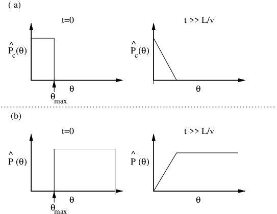
For example, in the case of the billiard in Fig. 1(a), the angular deflection for small $\theta$ is typically of order $\theta^{1/2}$, which is much larger than $\theta$. In the case of the billiards in Fig. 1(b-d), a particle moving nearly parallel to a channel axis is scattered by an angle of order one. Furthermore, after a large deflection, the orientation of the particle’s velocity vector is rapidly randomized by a succession of many reflections which, since the particle is no longer in a long flight, occur in a relatively short time. These considerations lead us to a model for the cases in Figs. 1(a)-1(d) in which we adopt the model hypothesis that, when a particle in a long flight suffers a collision with a billiard wall, the orientation of its velocity vector is randomly scattered with uniform probability density in $[0,2\pi]$. We wish to determine the evolution from the initial condition (1) in the case $\theta_{\textrm{max}}\ll 1$. This initial distribution is equal to the initial distribution $P_{b}(\bar{x},\bar{y},\theta,0)=K$ for all $\theta$ minus the initial condition $P_{c}(\bar{x},\bar{y},\theta,0)=K$ for $\theta<\theta_{max}$ and $0$ otherwise. The distribution $P_{b}$ remains unchanged when it is evolved forward in time (it is an invariant distribution). Thus, to find the evolution from initial condition (1), we can determine the evolution from $P_{c}$, and then subtract it from $K$. The long time evolution from $P_{c}$ can be found by considering the time at which particles are scattered. Consider, for example, the billiard of Fig. 1(d), and a particle with a small initial $\theta_{o}$. Suppose the particle is located in the channel at a distance $\Delta x$ from the boundary of the channel with which it will collide [left or right vertical dashed line in Fig. 1(d)]. If $\Delta x<vt\sin\theta_{o}\cong vt\theta_{o}$, the particle scatters before time $t$; if $\Delta x>vt\theta_{o}$, it does not scatter. For particles in the channel, $\Delta x<W$, so every particle with $\theta_{o}>W/(vt)$ must have scattered at least once. We assume that $t>W/(v\theta_{max})\equiv t_{o}$. Since $\theta_{\textrm{max}}$ is small, the scattered particles contribute a small positive value of order $\theta_{\textrm{max}}$ to $\hat{P}_{c}(\theta,t)$ in $\theta$. Thus $\hat{P}_{c}(\theta,t)$ is small (i.e., of order $\theta_{\textrm{max}}$) for $\theta>W/vt$. For $\theta_{o}<\Delta x/(vt)$, $t>t_{o}$, the particle has not yet scattered. Assuming that the initial spatial distribution of particles in the channel is uniform, the fraction of particles with initial angle $\theta_{o}$ that have scattered is $\theta_{o}vt/W$. Thus

where we have neglected the small, order $\theta_{max}$, contribution to $\hat{P}_{c}(\theta,t)$ from scattered particles. Subtracting $\hat{P}_{c}$ from $\hat{P}_{b}$ as illustrated in Fig. 3, we obtain the time asymptotic form in Eq. (3).

We now consider the evolution of initial condition (1) in the billiard of Fig. 1(e) for orbits experiencing long flights, Fig. 2(b). When an orbit in a long flight encounters the channel wall it may experience either one reflection (Fig. 4(a)) or two reflections (Fig. 4(b)). A geometrical analysis Lee shows that for $\theta^{\prime}\ll 1$, the relation between the angle $\theta^{\prime}$ before the encounter and the angle $\theta$ after the encounter is $\theta\cong M(\epsilon)\theta^{\prime}$, where $\epsilon$ is the distance illustrated in Figs. 4(a,b) and $M(\epsilon)$ is the piecewise linear function shown in Fig. 4(c). Note from Fig. 4(c) that the trajectory angle can increase or decrease at most by a factor of $3$ upon an encounter with the wall. Thus a long flight is again followed by a long flight, in contrast to the billiards of Figs. 1(a-d). That is, the infinite flight invariant set for the billiard of Fig. 1(e) is more sticky than are those of the other billiards, Figs. 1(a-d). Note also that, for $\theta\ll 1$, $\epsilon$ at the next encounter with the end of the channel is very sensitive to a small percentage change in $\theta$. This fact, together with the form of $M(\epsilon)$ shown in Fig. 4(c), leads us to adopt a model for our subsequent analysis whereby upon an encounter with the wall $\theta^{\prime}\to\theta=M\theta^{\prime}$ where $M$ is chosen randomly with uniform probability density in the interval $(1/3,3)$. As previously noted $S_{1}(\phi)\equiv 0$ for $\phi<1/2$. This can be understood as follows. $\hat{P}(\theta,0)=0$ for $\theta<\theta_{0}$, and on subsequent wall encounters $\theta$ can decrease at most by a factor of $3$. Therefore, after $n$ encounters the minimum angle is $\theta_{n}=\theta_{0}/3^{n}$ and the minimum time for these $n$ encounters is $t_{n}=\sum_{n^{\prime}=0}^{n-1}W/(v\theta_{n^{\prime}})\approx(W/v)3^{n}/(2\theta_{0})$ for $n\gg 1$, yielding a minimum value of $1/2$ for $\phi$.

Let $Q(\theta,t)\mathrm{d}\theta$ be the rate at which particles are scattered into the channel with angle between $\theta$ and $\theta+\mathrm{d}\theta$. Particles that enter the channel with small angle $\theta$ remain in the channel for the time $W/(v\sin\theta)\cong W/(v\theta)$. Then for large $t$ and small $\theta$, since the number of particles in the interval $\theta$ to $\theta+\mathrm{d}\theta$ at time $t$ is approximately $S_{1}(\phi)\mathrm{d}\theta$, we have $S_{1}(\phi)=\int_{t-W/(v\theta)}^{t}Q(\theta,t^{\prime})\mathrm{d}t^{\prime}$. Since the left hand side is only a function of $\phi$, $Q(\theta,t)$ must have the asymptotic scaling form $Q(\theta,t)=(v\theta/W)C(\phi)$. Thus

To obtain an equation for $C(\phi)$ consider a particle in a long flight that, at time $t^{\prime}$, has just suffered an encounter with a channel wall. Denote its angle as a result of this encounter by $\theta^{\prime}\ll 1$ (see Figs. 4(a,b)). The particle then experiences a long flight of duration $W/(v\theta^{\prime})$ before it next encounters a channel wall. According to our model, the velocity angle $\theta$ just after this encounter at time $t$ is $\theta=M\theta^{\prime}$ where $M$ is random with uniform probability density in the interval $(1/3,3)$. During a time interval $t$ to $t+\mathrm{d}t$ the number of particles scattered into the interval $\theta$ to $\theta+\mathrm{d}\theta$ is $Q(\theta,t)\mathrm{d}\theta\mathrm{d}t=3/8\int_{1/3}^{3}\left[Q(\theta^{\prime},t^{\prime})\mathrm{d}\theta^{\prime}\mathrm{d}t^{\prime}\right]\mathrm{d}M$, where $\theta^{\prime}=\theta/M$, $t^{\prime}=t-\frac{W}{v\theta^{\prime}}$, and $3/8=1/(3-1/3)$ is the probability density of the random variable $M$. Now substituting $Q(\theta,t)=(v\theta/W)C(\phi)$ and making a change of the integration variable $m=1/M$, we arrive at the following integral equation for $C(\phi)$,

whose solution along with (5) determines $S_{1}$. We numerically solve (6) by iteration of $C_{i+1}(\phi)=\mathcal{L}[C_{i}(\phi)]$ starting with $C_{0}(\phi)=0$ if $\phi<1$ and $C_{0}(\phi)=1$ if $\phi\geq 1$. We use $10^{4}$ grid points uniformly spaced in the $\phi$ interval $[0,50]$ with $C_{i}(\phi)$ set to one for $\phi>50$ (this corresponds to the boundary condition $C(\phi)\to\mathrm{const.}$ for $\phi\to\infty$). The results are virtually unchanged if the $\phi$ interval is increased to $[0,100]$ or if the number of grid points is increased, and virtually identical results (i.e., convergence) were found for several $i>12$. A result obtained from such a calculation is shown as the solid curve in Fig. 2 $(i=15)$ and is in good agreement with our numerical histograms computed from many particle orbits AHO1.

In conclusion, we have shown that the long-time repopulation of long flights in infinite horizon billiards proceeds in a self-similar manner [Eq. (2)]. The corresponding relaxation of the distribution [which follows from (2)] is algebraic rather than exponential; e.g., the $\theta$ integral of $|\hat{P}(\theta,t)-\hat{P}(\theta,\infty)|$ decays like $1/t$. Furthermore, the self-similar forms found for a class of billiards that include those of Figs. 1(a-d) are the same, Eq. (3). On the other hand, the special case of the billiard of Fig. 1(e) is shown to yield a different time-asymptotic self-similar form, and this may be ascribed to the greater stickiness of the invariant set of this billiard.

We thank J. R. Dorfman for discussions. This work was supported by the Office of Naval Research (Physics) and by the National Science Foundation (Grants PHYS098632, DMS010487).

References

- (1) T. Geisel, A. Zacherl, and G. Radons, Phys. Rev. Lett 59, 2503 (1987).
- (2) L. A. Bunimovich and Ya. G. Sinai, Commun. Math. Phys. 78:479 (1981).
- (3) L. A. Bunimovich, Commun. Math. Phys. 65,295 (1979).
- (4) P. M. Bleher J. Stat. Phys. 66:315 (1992).
- (5) K.C. Lee, Phys. Rev. Lett. 60:1991 (1988).
- (6) V. V. Afanasiev, R. Z. Sagdeev and G. M. Zaslavsky, Chaos 1, 149 (1991).
- (7) Levy Flights and Related Topics in Physics, edited by M. Shlesinger, G. M. Zaslavsky, and U. Frisch (Springer-Verlag, Heidelberg, 1995).
- (8) The implications of this result for deviation from classical diffusive behavior will be treated in a future publication [D. N. Armstead, B. R. Hunt, and E. Ott http://arXiv.org/abs/nlin.CG/0210062].
- (9) M. F. Shlesinger, Annu. Rev. Phys. Chem. 39, 269 (1988).
- (10) G. M. Zaslavsky and M. Edelman, Chaos 10, 135 (2000).
- (11) G. Zumofen and J. Klafter, Phys. Rev. E 47, 851 (1993).
- (12) R. Ishizaki, T. Horita, T. Kobayashi and H. Mori, Prog. Theor. Phys. 85, 1013 (1991).
- (13) S. Benkadda, S. Kassibrakis, R. B. White and G. M. Zaslavsky, Phys. Rev. E 55, 4909 (1997).
- (14) C. F. F. Karney, Physica D 8, 360 (1983).
- (15) J. D. Hanson, J. R. Cary and J. D. Meiss, J. Stat. Phys. 39, 327 (1985).
- (16) J. D. Meiss and E. Ott, Phys. Rev. Lett. 55, 2741 (1984); M. Ding, T. Bountis and E. Ott, Phys. Lett. A 151, 395 (1990).
- (17) In a future publication we also solve (6) using a power series expansion in again obtaining good agreement with our numerical histograms [D. N. Armstead, B. R. Hunt, and E. Ott (to be published)].