Chaotic Field Theory: a Sketch

Field theories such as 4-dimensional QCD or gravity have many dimensions, symmetries, tensorial indices. They are far too complicated for exploratory forays into this forbidding terrain. We start instead by taking a simple spatio-temporally chaotic nonlinear system of physical interest, and investigate the nature of its solutions.

One of the simplest and extensively studied spatially extended dynamical systems is the Kuramoto-Sivashinsky system [6]

which arises as an amplitude equation for interfacial instabilities in a variety of contexts. The “flame front” $u(x,t)$ has compact support, with $x\in[0,2\pi]$ a periodic space coordinate. The $u^{2}$ term makes this a nonlinear system, $t$ is the time, and $\nu$ is a fourth-order “viscosity” damping parameter that irons out any sharp features. Numerical simulations demonstrate that as the viscosity decreases (or the size of the system increases), the “flame front” becomes increasingly unstable and turbulent. The task of the theory is to describe this spatio-temporal turbulence and yield quantitative predictions for its measurable consequences.

Armed with a computer and a great deal of skill, one can obtain a numerical solution to a nonlinear PDE. The real question is; once a solution is found, what is to be done with it? The periodic orbit theory is an answer to this question.

Dynamics drives a given spatially extended system through a repertoire of unstable patterns; as we watch a “turbulent” system evolve, every so often we catch a glimpse of a familiar pattern:

    $\Longrightarrow$    other swirls    $\Longrightarrow$    

For any finite spatial resolution, the system follows approximately for a finite time a pattern belonging to a finite alphabet of admissible patterns, and the long term dynamics can be thought of as a walk through the space of such patterns, just as chaotic dynamics with a low dimensional attractor can be thought of as a succession of nearly periodic (but unstable) motions. The periodic orbit provides the machinery that converts this intuitive picture into precise calculation scheme that extracts asymptotic time predictions from the short time dynamics. For extended systems the theory gives a description of the asymptotics of partial differential equations in terms of recurrent spatio-temporal patterns.

Putkaradze has proposed that the Kuramoto-Sivashinsky system (1) be used as a laboratory for exploring such ideas. We now summarize the results obtained so far in this direction by Christiansen et al. [7] and Zoldi and Greenside [8].

The solution $u(x,t)=u(x+2\pi,t)$ is periodic on the $x\in[0,2\pi]$ interval, so one (but by no means only) way to solve such equations is to expand $u(x,t)$ in a discrete spatial Fourier series

Restrict the consideration to the subspace of odd solutions $u(x,t)=-u(-x,t)$ for which $a_{k}$ are real. Substitution of (2) into (1) yields the infinite ladder of evolution equations for the Fourier coefficients $a_{k}$:

$u(x,t)=0$ is a fixed point of (1), with the $k^{2}\nu<1$ long wavelength modes of this fixed point linearly unstable, and the short wavelength modes stable. For $\nu>1$, $u(x,t)=0$ is the globally attractive stable fixed point; starting with $\nu=1$ the solutions go through a rich sequence of bifurcations, and myriad unstable periodic solutions whose number grows exponentially with time.

The essential limitation on the numerical studies undertaken so far have been computational constraints: in truncation of high modes in the expansion (3), sufficiently many have to be retained to ensure the dynamics is accurately represented. Christiansen et al. [7] have examined the dynamics for values of the damping parameter close to the onset of chaos, while Zoldi and Greenside [8] have explored somewhat more turbulent values of $\nu$. With improvement of numerical codes considerably more turbulent regimes should become accessible.

One pleasant surprise is that even though one is dealing with (infinite dimensional) PDEs, for these strong dissipation values of parameters the spatio-temporal chaos is sufficiently weak that the flow can be visualised as an approximately 1-dimensional Poincaré return map $s\rightarrow f(s)$ from the unstable manifold of the shortest periodic point onto its neighborhood, see figure 1(a). This representation makes it possible to systematically determine all nearby periodic solutions up to a given maximal period.

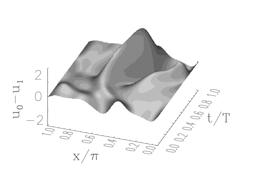
So far some 1,000 prime cycles have been determined numerically for various values of viscosity. The rapid contraction in the nonleading eigendirections is illustrated in figure 1(b) by the plot of the first 16 eigenvalues of the $\overline{1}$-cycle. As the length of the orbit increases, the magnitude of contracting eigenvalues falls off very quickly. In figure 2 we plot $u_{0}(x,t)$ corresponding to the $\overline{0}$-cycle. The difference between this solution and the other shortest period solution is of the order of 50% of a typical variation in the amplitude of $u(x,t)$, so the chaotic dynamics is already exploring a sizable swath in the space of possible patterns even so close to the onset of spatio-temporal chaos. Other solutions, plotted in the configuration space, exhibit the same overall gross structure. Together they form the repertoire of the recurrent spatio-temporal patterns that is being explored by the turbulent dynamics.

Now we turn to the central issue; qualitatively, these solutions demonstrate that the recurrent patterns program can be implemented, but how is this information to be used quantitatively? This is what the periodic orbit theory is about; it offers the machinery that assembles the topological and the quantitative information about individual solutions into accurate predictions about measurable global averages, such as the Lyapunov exponents and correlation functions.

Very briefly (for a detailed exposition the reader is referred to ref. [9]), the task of any theory that aspires to be a theory of chaotic, turbulent systems is is to predict the value of an “observable” $a$ from the spatial and time averages evaluated along dynamical trajectories $x(t)$

The key idea of the periodic orbit theory is to extract this average from the leading eigenvalue of the evolution operator

via the trace formula

$${\rm tr}\,{{\mathcal{L}}}^{t}=\sum_{p}\left.\raisebox{-17.22217pt}[23.68048pt][19.37494pt]{\includegraphics[height]{traceTube.eps}}\right._{p}=\sum_{p}\sum_{r=1}^{\infty}{{T_{p}}\,\delta\negthinspace\left({t-r{T_{p}}}\right)\over\left|\mbox{\rm det}\left({\bf 1}-{\bf J}_{p}^{r}\right)\right|}\e^{r\beta A_{p}}$$

(4)

which relates the spectrum of the evolution operator to a sum over prime periodic solutions $p$ of the dynamical system and their repeats $r$.

What does this formula mean? Prime cycles partition the dynamical space into neighborhoods, each cycle enclosed by a tube whose volume is the product of its length ${T_{p}}$ and its thickness $\left|\mbox{\rm det}({\bf 1}-{\bf J}_{p})\right|^{-1}$. The trace picks up a periodic orbit contribution only when the time $t$ equals a prime period or its repeat, a constraint enforced here by $\delta\negthinspace\left({t-r{T_{p}}}\right)$. ${\bf J}_{p}$ is the linear stability of cycle $p$, so for long cycles $\left|\mbox{\rm det}\left({\bf 1}-{\bf J}_{p}^{r}\right)\right|\approx$ (product of expanding eigenvalues), and the contribution of long and very unstable cycles are exponentially small compared to the short cycles which dominate trace formulas. The number of contracting directions and the overall dimension of the dynamical space is immaterial; that is why the theory can also be applied to PDEs. All this information is purely geometric, intrinsic to the flow, coordinate reparametrization invariant, and the same for any average one might wish to compute. The information related to a specific observable is carried by the weight $\e^{\beta A_{p}}$, the periodic orbit estimate of the contribution of $\e^{\beta A^{t}(x)}$ from the $p$-cycle neighborhood.

The intuitive meaning of a trace formula is that it expresses the average $\left<\e^{\beta A^{t}}\right>$ as a discretized integral

${{\mbox{smooth}\atop\mbox{dynamics}}~~~~~~~~\hskip-17.22217pt\includegraphics[width]{f_1_08_1.ps}\hskip-17.22217pt~~~~~~~~{\mbox{linearized}\atop\mbox{neighborhoods}}}$

over the dynamical space partitioned topologically into a repertoire of spatio-temporal patterns, each weighted by the likelihood of pattern’s occurrence in the long time evolution of the system.

Periodic solutions are important because they form the skeleton of the invariant set of the long time dynamics, with cycles ordered hierarchically; short cycles give good approximations to the invariant set, longer cycles refinements. Errors due to neglecting long cycles can be bounded, and for nice hyperbolic systems they fall off exponentially or even super-exponentially with the cutoff cycle length [10]. Short cycles can be accurately determined and global averages (such as Lyapunov exponents and escape rates) can be computed from short cycles by means of cycle expansions.

The Kuramoto-Sivashinsky periodic orbit calculations of Lyapunov exponents and escape rates [7] demonstrate that the periodic orbit theory predicts observable averages for deterministic but classically chaotic spatio-temporal systems. The main problem today is not how to compute such averages — periodic orbit theory as well as direct numerical simulations can handle that — but rather that there is no consensus on what the sensible experimental observables worth are predicting.

It should be obvious, and it still needs to be said: the spatio-temporally periodic solutions are not to be thought of as eigenmodes, a good linear basis for expressing solutions of the equations of motion. Something like a dilute instant approximation makes no sense at all for strongly nonlinear systems that we are considering here. As the equations are nonlinear, the periodic solutions are in no sense additive, and their linear superpositions are not solutions.

${A\raisebox{-17.22217pt}[23.68048pt][19.37494pt]{ \includegraphics[height]{solution1.eps} }~+~B\raisebox{-17.22217pt}[23.68048pt][19.37494pt]{ \includegraphics[height]{solution2.eps} }+\,\,\cdots\quad\neq\mbox{~~~{u(x,t)}}\atop\mbox{~~~~~~~~~~~a solution ~~~~~~~~~~~~~~ a solution ~~~~~~~~~~~ not a solution}}$

Instead, it is the trace formulas and spectral determinants of the periodic orbit theory that prescribe how the repertoire of admissible spatio-temporal patterns is to be systematically explored, and how these solutions are to be put together in order to predict measurable observables.

Suppose that the above program is successfully carried out for classical solutions of some field theory. What are we to make of this information if we are interested in the quantum behavior of the system? In the semiclassical quantization the classical solutions are the starting approximation.

For the same pragmatic reasons that we found it profitable to shy away from facing the 4-dimensional QCD head on in the above exploratory foray into a strongly nonlinear field theory, we shall start out by trying to understand the structure of perturbative corrections for systems radically simpler than a full-fledged quantum field theory. First, instead of perturbative corrections to the quantum problem, we shall start by exploring the perturbative corrections to weakly stochastic flows. Second, instead of continuous time flows, we shall start by a study of a discrete time process.

For discrete time dynamics a Langevin trajectory in presence of additive noise is generated by iteration

where $f(x)$ is a map, $\xi_{n}$ a random variable, and $\sigma$ parametrizes the noise strength. In what follows we assume that $\xi_{n}$ are uncorrelated, and that the mapping $f(x)$ is one-dimensional and expanding, but we expect that the form of the results will remain the same for higher dimensions, including the field theory example of the preceding section.

Tracking an individual noisy trajectory does not make much sense; what makes sense is the Fokker-Planck formulation, where one considers instead evolution of an ensemble of trajectories. An initial density of trajectories $\phi_{0}(x)$ evolves with time as

where ${\mathcal{L}}$ is the evolution operator

and $\xi_{n}$ a random variable with the normalized distribution $P(\xi)$, centered on $\xi=0$.

If the noise is weak, the goal of the theory is to compute the perturbative corrections to the eigenvalues ${\nu}$ of ${\mathcal{L}}$ order by order in the noise strength $\sigma$,

One way to get at the spectrum of ${\mathcal{L}}$ is to consider the discrete Laplace transform of ${\mathcal{L}}^{n}$, or the resolvent

which has a pole at every $z={\nu}_{\alpha}^{-1}$.

The effects of weak noise are of interest in their own right, as any deterministic evolution that occurs in nature is affected by noise. However, what is most important in the present context is the fact that the form of perturbative corrections for the stochastic problem is the same as for the quantum problem, and still the actual calculations are sufficiently simple that one can explore many more orders in perturbation theory than would be possible for a full-fledged field theory, and develop new perturbative methods.

The first method we try is the standard Feynman-diagrammatic expansion. For semiclassical quantum mechanics of a classically chaotic system such calculation was first carried out by Gaspard [11]. The stochastic version described here, implemented by Dettmann [12], reveals features not so readily apparent in the quantum calculation.

The Feynman diagram method becomes unwieldy at higher orders. The second method, introduced by Vattay [13], is based on Rugh’s [10] explicit matrix representation of the evolution operator. If one is interested in evaluating numerically many orders of perturbation theory and many eigenvalues, this method is unsurpassed.

The third approach, the smooth conjugations introduced by Mainieri [14], is perhaps an altogether new idea in field theory. In this approach the neighborhood of each saddlepoint is rectified by an appropriate nonlinear field transformation, with the focus shifted from the dynamics in the original field variables to the properties of the conjugacy transformation. The expressions obtained are equivalent to sums of Feynman diagrams, but are more compact.

We start our computation of the weak noise corrections to the spectrum of ${\mathcal{L}}$ by calculating the trace of the $n$-th iterate of the stochastic evolution operator ${\mathcal{L}}$. A convenient choice of noise is Gaussian, $P(\xi)=e^{-\xi^{2}/2}/{\sqrt{2\pi}}\,,$ with the trace given by an $n$-dimensional integral on $n$ points along a discrete periodic chain

The choice of Gaussian noise is not essential, as the methods that we develop here apply equally well to other noise distributions, and more generally to the space dependent noise distributions $P(x,\xi)$. As the neighborhood of any trajectory is nonlinearly distorted by the flow, the integrated noise is anyway never Gaussian, but colored.

If the classical dynamics is hyperbolic, periodic solutions of given finite period $n$ are isolated. Furthermore, if the noise broadening $\sigma$ is sufficiently weak they remain distinct, and the dominant contributions come from neighborhoods of periodic points, the tubes sketched in the trace formula (4). In the saddlepoint approximation the trace (9) is given by the sum over neighborhoods of periodic points

As traces are cyclic, $e^{W_{c}}$ is the same for all periodic points in a given cycle, independent of the choice of the starting point $x_{c}$, and the periodic point sum can be rewritten in terms of prime cycles $p$ and their repeats. In the deterministic, $\sigma\to 0$ limit this is the discrete time version of the classical trace formula (4). Effects such as noise induced tunnelling are not included in the weak noise approximation.

We now turn to the evaluation of $W_{p^{r}}$, the weight of the $r$-th repeat of prime cycle $p$. The contribution of the cycle point $x_{a}$ neighborhood is best expressed in an intrinsic coordinate system, by centering the coordinate system on the cycle points,

From now on $x_{a}$ will refer to the position of the $a$-th periodic point, $\phi_{a}$ to the deviation of the noisy trajectory from the deterministic one, $f_{a}(\phi_{a})$ to the map (5) centered on the $a$-th cycle point, and $f_{a}^{(m)}$ to its $m$-th derivative evaluated at the $a$-th cycle point:

Rewriting the trace in vector notation, with $x$ and $f(x)$ $n$-dimensional column vectors with components $x_{a}$ and $f(x_{a})$ respectively, expanding $f$ in Taylor series around each of the periodic points in the orbit of $x_{c}$, separating out the quadratic part and integrating we obtain

The [$n$$\times$$n$] matrix $\Delta$ arises from the quadratic part of the exponent, while all higher powers of $\phi_{a}$ are collected in $V(\phi)$:

The saddlepoint expansion is most conveniently evaluated in terms of Feynman diagrams, by drawing $\Delta$ as a directed line $\Delta_{ab}=\raisebox{-8.61108pt}[15.0694pt][10.76385pt]{\includegraphics[height]{Delta.eps}\negthinspace}$, and the derivatives of $V$ as the “interaction” vertices ¹¹ 1 PC: fix birdtrack height

$$f^{{}^{\prime\prime}}_{a}\,=\,\raisebox{-8.61108pt}[15.0694pt][10.76385pt]{\includegraphics[height]{f2.eps}\negthinspace}\,,\quad f^{{}^{\prime\prime\prime}}_{a}\,=\,\raisebox{-8.61108pt}[15.0694pt][10.76385pt]{\includegraphics[height]{f3.eps}\negthinspace}\,,\quad\dots\,.$$

In the jargon of field theory, $\Delta$ is the “free propagator”. Its determinant

is the 1-dimensional version of the classical stability weight $\left|\mbox{\rm det}({\bf 1}-{\bf J})\right|^{-1}$ in (4), with $\Lambda_{c}$ the stability of the $n$-cycle going through the periodic point $x_{c}$.

Standard methods [15] now yield the perturbation expansion in terms of the connected “vacuum bubbles”

	$\displaystyle W_{c}$	$\displaystyle=$	$\displaystyle-\ln|\Lambda_{c}-1|+\sum_{k=1}^{\infty}W_{c,2k}\sigma^{2k}$		(16)
	$\displaystyle W_{c,2}$	$\displaystyle=$	$\displaystyle{1\over 2}\,\raisebox{-8.61108pt}[15.0694pt][10.76385pt]{\includegraphics[height]{FeynmDumb1.eps}\negthinspace}\,+\,{1\over 2}\,\raisebox{-8.61108pt}[15.0694pt][10.76385pt]{\includegraphics[height]{FeynmDumb2.eps}\negthinspace}\,+\,{1\over 2}\,\raisebox{-8.61108pt}[15.0694pt][10.76385pt]{\includegraphics[height]{FeynmEight.eps}\negthinspace}\,+\,{1\over 2}\,\raisebox{-8.61108pt}[15.0694pt][10.76385pt]{\includegraphics[height]{FeynmLips.eps}\negthinspace}$
	$\displaystyle W_{c,4}$	$\displaystyle=$	$\displaystyle\cdots\,.$

In the usual field-theoretic calculations the $W_{c,0}$ term corresponds to an overall volume term that cancels out in the expectation values. In contrast, as explained in sect. 2, here the $e^{W_{c,0}}=|\Lambda_{c}-1|^{-1}$ term is the classical volume of cycle $c$. Not only does this weight not cancel out in the expectation value formulas, it plays the key role both in classical and semiclassical trace formulas.

In the diagrams sketched above a propagator line connects $x_{a}$ at time $a$ with $x_{b}$ at later time $b$ by a deterministic trajectory. At time $b$ noise induces a kick whose strength depends on the local curvature of the flow. A penalty of a factor $\sigma$ is paid, $m-1$ deterministic trajectories originate in the neighborhood of $x_{b}$ from vertex $V^{(m)}(x_{b})$, and the process repeats itself, each vertex carrying a penalty of $\sigma$, and higher derivatives of the $f_{b}$. Summing over all noise kick sequences encoded by a given diagram and using the periodicity of the trace integral (9) Dettmann [12] obtains expressions such as

This particular sum is the Feynman diagram $\sigma^{2}$ correction to $r$-th repeat of prime cycle $p$. More algebra leads to similar contributions from the remaining diagrams. But the overall result is surprising; the dependence on the repeat number $r$ factorizes, with each diagram yielding the same prefactor depending only on $\Lambda_{p}^{r}$. This remarkable fact will be explained in sect. 6. The result of the Feynman-diagrammatic calculations is the stochastic trace formula

where $t_{p,k}$ is the $k$-th local eigenvalue evaluated on the $p$ cycle. The deterministic, $\sigma=0$ part of this formula is the stochastic equivalent of the Gutzwiller semiclassical trace formula [5]. The $\sigma^{2}$ correction $w_{p,k}^{(2)}$ is the stochastic analogue of Gaspard’s $\hbar$ correction [11]. At the moment the explicit formula is sufficiently unenlightening that we postpone writing it down to sect. 6.

While the diagrams are standard, the chaotic field theory calculations are considerably more demanding than is usually the case in field theory. Here there is no translational invariance along the chain, so the vertex strength depends on the position, and the free propagator is not diagonalized by a Fourier transform. Furthermore, here one is neither “quantizing” around a trivial vacuum, nor a countable infinity of analytically explicit soliton saddles, but around an infinity of nontrivial unstable hyperbolic saddles.

Two aspects of the above perturbative results are a priori far from obvious: (a) that the structure of the periodic orbit theory should survive introduction of noise, and (b) a more subtle and surprising result, repeats of prime cycles can be re-summed and theory reduced to the dynamical zeta functions and spectral determinants of the same form as for deterministic systems.

Pushing the Feynman-diagrammatic approach to higher orders is laborious, and has not been attempted for this class of problems. As we shall now see, it is not smart to keep pushing it, either, as one can compute many more orders of perturbation theory by means of a matrix representation for ${\mathcal{L}}$.

An expanding map $f(x)$ takes an initial smooth distribution $\phi(x)$ defined on a subinterval, stretches it out and overlays it over a larger interval. Repetition of this process smoothes the initial distribution $\phi(x)$, so it is natural to concentrate on smooth distributions $\phi_{n}(x)$, and represent them by their Taylor series. By expanding both $\phi_{n}(x)$ and $\phi_{n+1}(y)$ in (6) in Taylor series Rugh [10] derived a matrix representation of the evolution operator

which maps the $x^{m}$ component of the density of trajectories $\phi_{n}(x)$ in (6) to the $y^{m^{\prime}}$ component of the density $\phi_{n+1}(y)$ one time step later. The matrix elements follow by differentiating both sides with $\partial^{m^{\prime}}/\partial y^{m^{\prime}}$ and evaluating the integral

In (7) we have written the evolution operator ${\mathcal{L}}$ in terms of the Dirac delta function in order to emphasize that in the weak noise limit the stochastic trajectories are concentrated along the classical trajectory $y=f(x)$. Hence it is natural to expand the kernel in a Taylor series  [17] in $\sigma$

where $\delta^{(n)}(y)={\partial^{n}\over\partial y^{n}}\delta(y)\,.$ This yields a representation of the evolution operator centered along the classical trajectory, dominated by the deterministic Perron-Frobenius operator $\delta(y-f(x))$, with corrections given by derivatives of delta functions weighted by moments of the noise distribution $P_{n}=\int P(\xi)\xi^{n}d\xi$. We again center the coordinate system on the cycle points as in (11), and also introduce a notation for the operator (7) centered on the $x_{a}\to x_{a+1}$ segment of the classical trajectory

The weak noise expansion (20) for the $a$-th segment operator is given by

As the evolution operator has a simple $\delta$-function form, the local matrix representation of ${\mathcal{L}}_{a}$ centered on the $x_{a}\to x_{a+1}$ segment of the deterministic trajectory can be evaluated recursively in terms of derivatives of the map $f$:

The matrix elements vanish for $m^{\prime}<m$, so ${{\bf B}}$ is a lower triangular matrix. The diagonal and the successive off-diagonal matrix elements are easily evaluated iteratively by computer algebra

For chaotic systems the map is expanding, $|f_{a}^{\prime}|>1$. Hence the diagonal terms drop off exponentially, as $1/|f_{a}^{\prime}|^{m+1}$, the terms below the diagonal fall off even faster, and truncating ${{\bf L}_{a}}$ to a finite matrix introduces only exponentially small errors.

The trace formula (8) takes now a matrix form

where ${{\bf L}_{p}}={{{\bf L}_{{n_{p}}}}{{\bf L}_{2}}\cdots{{\bf L}_{1}}}$ is the contribution of the $p$ cycle. The subscript sc is a reminder that this is a saddlepoint or semiclassical approximation, valid as an asymptotic series in the limit of weak noise. Vattay [16] interprets the local matrix representation of the evolution operator as follows. The matrix identity log det = tr log together with the trace formula (23) yields

so in the saddlepoint approximation the spectrum of the global evolution operator ${\mathcal{L}}$ is pieced together from the local spectra computed cycle-by-cycle on neighborhoods of individual prime cycles with periodic boundary conditions. The meaning of the $k$-th term in the trace formula (18) is now clear; it is the $k$-th eigenvalue of the local evolution operator restricted to the $p$-th cycle neighborhood.

Using this matrix representation Palla and Søndergaard [13] were able to compute corrections to order $\sigma^{12}$, a feat simply impossible along the Feynman-diagrammatic line of attack. In retrospect, the matrix representation method for solving the stochastic evolution is eminently sensible — after all, that is the way one solves a close relative to stochastic PDEs, the Schrödinger equation. What is new is that the problem is being solved locally, periodic orbit by periodic orbit, by translation to coordinates intrinsic to the periodic orbit. It is this natural local basis that makes the matrix representation so simple.

Mainieri [14] takes this observation one step further; as the dynamics is nonlinear, why not search for a nonlinear coordinate transformation that makes the intrinsic coordinates as simple as possible?

This step injects into field theory a method standard in the construction of normal forms for bifurcations [18]. The idea is to perform a smooth nonlinear coordinate transformation $x=h(y)$, $f(x)=h(g(h^{-1}(x)))$ that flattens out the vicinity of a fixed point and makes the map linear in an open neighborhood, $f(x)\to g(y)={\bf J}\cdot y$.

${\raisebox{-17.22217pt}[23.68048pt][19.37494pt]{ \includegraphics[height]{conjug-a.eps} }\atop\mbox{an arbitrary coordinatization}}$     $\Longrightarrow$     ${\raisebox{-17.22217pt}[23.68048pt][19.37494pt]{ \includegraphics[height]{conjug-b.eps} }\atop\mbox{intrinsic, flat coordinates}}$

The key idea of flattening the neighborhood of a saddlepoint can be traced back to Poincaré’s celestial mechanics, and is perhaps not something that a field theorist would instinctively hark to as a method of computing perturbative corrections. This local rectification of a map can be implemented only for isolated non-degenerate fixed points (otherwise higher terms are required by the normal form expansion around the point), and only in finite neighborhoods, as the conjugating functions in general have finite radia of convergence.

We proceed in two steps. First, substitution of the weak noise perturbative expansion of the evolution operator (21) into the trace centered on cycle $c$ generates products of derivatives of $\delta$-functions:

The integrals are evaluated as in (22), yielding recursive derivative formulas such as

or $n$-point integrals, with derivatives distributed over $n$ different $\delta$-functions.

Next we linearize the neighborhood of the $a$-th cycle point. For a 1-dimensional map $f(x)$ with a fixed point $f(0)=0$ of stability $\Lambda=f^{\prime}(0)$, $|\Lambda|\neq 1$ we search for a smooth conjugation $h(x)$ such that:

In higher dimensions $\Lambda$ is replaced by the Jacobian matrix ${\bf J}$. For a periodic orbit each point around the cycle has a differently distorted neighborhood, with differing second and higher derivatives, so the conjugation function $h_{a}$ has to be computed point by point,

An explicit expression for $h_{a}$ in terms of $f$ is obtained by iterating around the whole cycle, and using the chain rule (15) for the cycle stability $\Lambda_{p}$

so each $h_{a}$ is given by some combination of $f_{a}$ derivatives along the cycle. Expand $f(x)$ and $h(x)$

and equate recursively coefficients in the functional equation $h(\Lambda y)=f(h(y))$ expansion

This yields the expansion for the conjugation function $h$ in terms of the mapping $f$

The periodic orbit conjugating functions $h_{a}$ are obtained in the same way from (27), with proviso that the cycle stability is not marginal, $|\Lambda_{p}|\neq 1$.

What is gained by replacing the perturbation expansion in terms of $f^{(m)}$ by still messier perturbation expansion for the conjugacy function $h$? Once the neighborhood of a fixed point is linearized, the conjugation formula for the repeats of the map

can be used to compute derivatives of a function composed with itself $r$ times. The expansion for arbitrary number of repeats depends on the conjugacy function $h(x)$ computed for a single repeat, and all the dependence on the repeat number is carried by polynomials in $\Lambda^{r}$, a result that emerged as a surprise in the Feynman diagrammatic approach of sect. 4. The integrals such as (25) evaluated on the $r$-th repeat of prime cycle $p$

have a simple dependence on the conjugating function $h$

The evaluation of $n$-point integrals is more subtle [14]. The final result of all these calculations is that expressions of form (31) depend on the conjugation function determined from the iterated map, with the saddlepoint approximation to the spectral determinant given by

in terms of local $p$-cycle eigenvalues

accurate up to order $\sigma^{4}$. $w^{(3)}$, $w^{(4)}$ are also computed by Dettmann, but we desist from citing them here; the reader is referred to ref. [14]. What is remarkable about these results is their simplicity when expressed in terms of the conjugation function $h$, as opposed to the Feynman diagram sums, in which each diagram contributes a sum like the one in (17), or worse. Furthermore, both the conjugation and the matrix approaches are easily automatized, as they require only recursive evaluation of derivatives, as opposed to the handcrafted Feynman diagrammar.

Simple minded as they might seem, discrete stochastic processes are a great laboratory for testing ideas that would otherwise be hard to test. Dettmann, Palla and Søndergaard have used a 1-dimensional repeller of bounded nonlinearity and complete binary symbolic dynamics to check numerically the above results, and computed the leading eigenvalue of ${\mathcal{L}}$ by no less than five different methods. As anticipated by Rugh [10], the evolution operator eigenvalues converge super-exponentially with the cycle length; addition of cycles of period $(n$+1$)$ to the set of all cycles up to length $n$ doubles the number of significant digits in the perturbative prediction. However, as the series is asymptotic, for realistic values of the noise strength summations beyond all orders are needed [19].

The periodic orbit theory approach to turbulence is to visualize turbulence as a sequence of near recurrences in a repertoire of unstable spatio-temporal patterns. The investigations of the Kuramoto-Sivashinsky system discussed above are first steps in the direction of implementing this program. So far, existence of a hierarchy of spatio-temporally periodic solutions of spatially extended nonlinear system has been demonstrated, and the periodic orbit theory has been tested in evaluation of global averages for such system. The parameter ranges tested so far probe the weakest nontrivial “turbulence”, and it is an open question to what extent the approach remains implementable as the system goes more turbulent.

The most important lesson of this investigation is that the unstable spatio-temporally periodic solutions do explore systematically the repertoire of admissible spatio-temporal patterns, with the trace and spectral determinants formulas and their cycle expansions being the proper tools for extraction of quantitative predictions from the periodic orbits data.

We formulat next a semiclassical perturbation theory for stochastic trace formulas with support on infinitely many chaotic saddles. The central object of the periodic orbit theory, the trace of the evolution operator, is a discrete path integral, similar to those found in field theory and statistical mechanics. The weak noise perturbation theory, likewise, resembles perturbative field theory, and can be cast into the standard field-theoretic language of Feynman diagrams. However, we found out that both the matrix and the nonlinear conjugacy perturbative methods are superior to the standard approach. In contrast to previous perturbative expansions around vacua and instanton solutions, the location and local properties of each saddlepoint must be found numerically.

The key idea in the new formulation of perturbation theory is this: Instead of separating the action into quadratic and “interaction” parts, one first performs a nonlinear field transformation which turns the saddle point into an exact quadratic form. The price one pays for this is the Jacobian of the nonlinear field transformation — but it turns out that the perturbation expansion of this Jacobian in terms of the conjugating function is order-by-order more compact than the Feynman-diagrammatic expansion.

I am indebted to my collaborators C.P. Dettmann, G. Vattay, F. Christiansen, V. Putkaradze, G. Palla, N. Søndergaard, R. Mainieri and H.H. Rugh for co-suffering through all the details omitted in this overview. I am grateful to E.A. Spiegel, L. Tuckerman and M.J. Feigenbaum for patient instruction. I am not grateful to those directors and gentlemen of committees who do not find theoretical physics a vibrant subject.

References

- [1] V.W. Hughes and T. Kinoshita, Rev. Mod. Phys. 71 (1999) S133.
- [2] R.S. Van Dyck, Jr., P.B. Schwinberg, H.G. Dehmelt, Phys. Rev. Lett. 59 (1987) 26.
- [3] K.G. Wilson, Phys. Rev. D 10 (1974) 2445.
- [4] A.A. Belavin, A.M. Polyakov, A.S. Swartz, Yu.S. Tyupkin, Phys. Lett. B 59 (1975) 85.
- [5] M.C. Gutzwiller, Chaos in Classical and Quantum Mechanics (Springer, New York 1990).
- [6]
Y. Kuramoto and T. Tsuzuki,
Progr. Theor. Physics 55 (1976) 365;
G.I. Sivashinsky, Acta Astr. 4 (1977) 1177. - [7] F. Christiansen, P. Cvitanović, V. Putkaradze, Nonlinearity 10 (1997) 1.
- [8] S.M. Zoldi and H.S. Greenside, Phys. Rev. E 57 (1998) R2511.
- [9] P. Cvitanović et al., Classical and Quantum Chaos (Niels Bohr Institute, Copenhagen 1999); www.nbi.dk/ChaosBook/.
- [10] H.H. Rugh, Nonlinearity 5 (1992) 1237.
- [11] P. Gaspard and D. Alonso, Phys. Rev. A 47 (1993) R3468.
- [12] P. Cvitanović, C.P. Dettmann, R. Mainieri, G. Vattay, J. Stat. Phys. 93 (1998) 981; chao-dyn/9807034.
- [13] P. Cvitanović, C.P. Dettmann, G. Palla, N. Søndergård, G. Vattay, Phys. Rev. E 60 (1999) 3936; chao-dyn/9904027.
- [14] P. Cvitanović, C.P. Dettmann, R. Mainieri, G. Vattay, Nonlinearity 12 (1999) 939; chao-dyn/9811003.
- [15]
P. Cvitanović,
Field theory
(Nordita, Copenhagen, 1983);
www.nbi.dk/predrag/field_the/. - [16]
G. Vattay and P.E. Rosenqvist,
Phys. Rev. Lett. 76 (1996) 335,
chao-dyn/9509015; G. Vattay, Phys. Rev. Lett. 76 (1996) 1059. - [17] S. Watanabe, Ann. of Prob. 15 (1987) 1.
- [18] See for example A. Katok and B. Hasselblatt, Introduction to the Modern Theory of Dynamical Systems (Cambridge University Press, Cambridge, 1995).
- [19] G. Palla, N. Søndergaard, G. Vattay, A. Voros, Trace formulas for stochastic evolution operators: Beyond all orders, in preparation.