A smooth space of tetrahedra

Let ${\mathbb{P}}^{n}$ be $n$-dimensional complex projective space, and let $P\subset{\mathbb{P}}^{n}$ be a set of $n+1$ labeled points in general position. By taking all possible linear spans of subsets of $P$, one obtains a configuration of flats in ${\mathbb{P}}^{n}$ arranged to form a simplex. The set $X^{\circ}$ of all such configurations is naturally a quasi-projective variety with a canonical singular compactification $X$. One is interested in the variety $X$ for many reasons:

• •

  For $n=2$, the space $X$ is the space of triangles in the plane. In [14], Schubert described a desingularization of $X$, and used it to study enumerative problems involving triangles [15, 13, 3].

• •

  The space $X$ is a configuration variety in the sense of Magyar [10, 18]. Such spaces arise naturally in the study of generalized Schur modules. These are (reducible) $\operatorname{GL}_{n}$-modules that generalize the classical Schur modules, and have been studied in various guises by many authors [1, 9, 19, 8, 11, 12, 16]. One hopes that configuration varieties will play a role in a Borel-Weil theory for these modules.

• •

  Let ${\mathscr{B}}$ be the Tits building for $\operatorname{SL}_{n+1}({\mathbb{C}})$, and let ${\mathscr{C}}$ be the associated Coxeter complex [17]. Then $X$ can be interpreted as the space of maps of ${\mathscr{C}}$ into ${\mathscr{B}}$. By considering other algebraic groups, one obtains a collection of natural configuration spaces related to the Bott-Samelson varieties of Demazure [4]. In particular, $X$ can be regarded as a canonical Bott-Samelson variety associated to all reduced expressions of the longest word of the Weyl group of $\operatorname{SL}_{n+1}$.

• •

  The space $X$ is a natural generalization of the Fulton-MacPherson space [5] ${\mathbb{P}}^{n}[n+1]$. This variety adds data to an open set of the product $\prod_{i=1}^{n+1}{\mathbb{P}}^{n}$ that records how points approach the (large) diagonals. In fact, ${\mathbb{P}}^{n}[n+1]$ is a desingularization of the space of all $1$-skeleta of $n$-simplices in ${\mathbb{P}}^{n}$.

In this paper we consider the case $n=3$, where $X$ is the space of tetrahedra in ${\mathbb{P}}^{3}$. We construct a symmetric compactification $\widetilde{X}$ of $X^{\circ}$ that we call the space of complete tetrahedra. It is obtained by embedding $X^{\circ}$ into a large ambient variety $E_{\#}$ and taking the closure of the image. The singular locus of the canonical compactification $X$ is contained in the subvariety consisting of “collapsed tetrahedra”—that is, configurations of flats where certain faces coincide (Figure 1)—and $E_{\#}$ is constructed to capture the asymptotic behavior of a tetrahedron as it collapses. Our main theorem (Theorem 7.6) is that $\widetilde{X}$ is nonsingular.

In a later paper [2] we will make a more detailed study of the geometry of $\widetilde{X}$. We will show that the complement of $X^{\circ}$ in $\widetilde{X}$ is a divisor with normal crossings and compute the cohomology ring of $\widetilde{X}$.

Although this article considers the space of tetrahedra in ${\mathbb{P}}^{3}$, the definition of $\widetilde{X}$ makes sense for all $n$. Many of the results of the paper (in particular, sections 4–6) hold for arbitrary $n$, but we have avoided this generality since we cannot complete the proof that $\widetilde{X}$ is nonsingular in general (the combinatorial arguments in section 7 become infeasible when $n\geq 4$). However, we conjecture that $\widetilde{X}$ provides a nonsingular compactification of $X^{\circ}$ for all $n$.

For $n=2$, it is not hard to see that our variety $\widetilde{X}$ is nonsingular and coincides with certain triangle varieties found in the literature. More precisely, it is isomorphic to the Fulton-MacPherson space ${\mathbb{P}}^{2}[3]$, which in turn coincides with an auxiliary compactification constructed by Roberts-Speiser [13]. It is not, however, isomorphic to Schubert’s compactification as a variety over $X$.¹¹ 1 The difference between Schubert’s space and Fulton-MacPherson-Roberts-Speiser’s space appears when one considers the torus action on them, cf. [18]

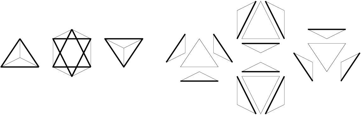
We now give an overview of the definition of $\widetilde{X}$. The construction of $E_{\#}$ depends on the combinatorics of hypersimplices [6], polytopes intimately related to the geometry of Grassmannians. For our considerations, the relevant polytopes are the $3$-dimensional hypersimplices $\Delta_{1}$, $\Delta_{2}$, and $\Delta_{3}$ (Figure 2). The vertices of these hypersimplices are in bijection with the labeled faces of a tetrahedron, and the edges of the hypersimplices correspond to certain pairs of faces of the same dimension.

For each edge $\alpha$ in a hypersimplex, we form a $({\mathbb{P}}^{1}\times{\mathbb{P}}^{1})$-bundle $E_{\alpha}\rightarrow X$. The bundle $E_{\alpha}$ has a canonical section $u_{\alpha}$ and a diagonal subbundle $D_{\alpha}$. The section $u_{\alpha}$ tracks the subspaces corresponding to the vertices of $\alpha$ in such a way that $u_{\alpha}$ intersects $D_{\alpha}$ precisely when these subspaces coincide. In order to record the asymptotic behavior in $X$ near a collapsed tetrahedron, a natural idea is to form products of the $E_{\alpha}$’s and blowup the corresponding product of diagonals. The question is which products to take, and why.

Our main idea is that the relevant products are those indexed by the faces of dimension $\geq 2$ of the hypersimplices. The motivation is that a configuration of flats in ${\mathbb{P}}^{3}$ arranged to form a tetrahedron contains certain “sub-” and “quotient” configurations corresponding to proper faces of the hypersimplices. For example, the three points and three lines in a given face of a tetrahedron form a subconfiguration that corresponds to a triangular face in the hypersimplex $\Delta_{1}$, and the three lines and three planes containing a given point form a quotient configuration that corresponds to a triangular face in the hypersimplex $\Delta_{3}$. Our motivation is that a nonsingular compactification of $X^{\circ}$ should add data recording the “infinitesimal shapes” of these sub- and quotient configurations. Hence, each locus we blowup corresponds to the collapsing together of the subspaces labeled by some face of a hypersimplex.

More precisely, our definition is as follows. Let ${\mathcal{H}}$ be the set of faces of dimension $\geq 2$ of all the $\Delta_{k}$. For each $\beta\in{\mathcal{H}}$, let ${\mathcal{E}}(\beta)$ be the set of edges in $\beta$. Let $E_{\beta}$ be the product bundle

and let $D_{\beta}$ be the corresponding product of the diagonals $D_{\alpha}$. The ambient variety $E_{\#}$ is then defined by blowing up each $E_{\beta}$ along $D_{\beta}$ and taking the product of the resulting blowups. The corresponding product of the sections $u_{\alpha}$, then determines an embedding $X^{\circ}\rightarrow E_{\#}$, and we define $\widetilde{X}$ to be the closure.

The paper is organized as follows. Section 2 sets up notation, defines $X$, and contains background on hypersimplices. Section 3 contains the construction of $E_{\#}$ and $\widetilde{X}$. In section 4 we describe a collection of affine open subvarieties that covers $X$ and give equations defining a typical element $U\subset X$ in this collection. In section 5 we restrict the construction of $E_{\#}$ to $U$ to obtain $\widetilde{U}$, a certain subvariety of $\widetilde{X}$. The point of sections 4–5 is that the nonsingularity of $\widetilde{X}$ follows from the nonsingularity of $\widetilde{U}$.

In the remaining sections we prove nonsingularity of $\widetilde{U}$. First, in section 6, we show that $\widetilde{U}$ has the structure of a vector bundle over a certain (multi-) projective variety ${Z}$ that we call the core. We then study the $\operatorname{GL}_{4}$-action on $\widetilde{U}$ to show that nonsingularity of ${Z}$ follows from its nonsingularity at points in a certain subvariety ${Z}_{sp}\subset{Z}$. Finally in section 7, we give equations that cut out ${Z}$ from projective space and use a graphical description of these defining relations to show that ${Z}_{sp}$ consists of nonsingular points of ${Z}$; this proves Theorem 7.6.

We thank Michael Thaddeus for suggesting the proof of Lemma 6.9. We thank Robert MacPherson, who originally told us about this problem, in terms of buildings and Coxeter complexes, and who has offered us much encouragement and interest. Finally, we thank the various institutions that have supported us and have hosted our collaboration at one time or another: Columbia University, Cornell University, the Institute for Advanced Study, the Ohio State University, and the University of Washington.

Let $e_{1},\dots,e_{4}$ be the standard basis of ${\mathbb{C}}^{4}$, and let $[\![4]\!]$ be the set $\{1,2,3,4\}$. For any subset $I\subset[\![4]\!]$, let $E_{I}\subset{\mathbb{C}}^{4}$ be the subspace spanned by $\{e_{i}\mid i\in I\}$. Let ${\mathbb{P}}^{3}$ be the projective space of lines in ${\mathbb{C}}^{4}$, and let $G$ be the algebraic group $\operatorname{GL}_{4}({\mathbb{C}})$.

For $k=1,2,3$, let $\operatorname{Gr}_{k}$ be the Grassmannian of $k$-dimensional subspaces of ${\mathbb{C}}^{4}$, and for each proper nonempty subset $I\subset[\![4]\!]$, let $\operatorname{Gr}_{I}:=\operatorname{Gr}_{|I|}$. (We use the notation $|I|$ for the cardinality of $I$.) Let $Y$ be the product

and for each $I\subset[\![4]\!]$, let $\pi_{I}$ be the projection to the $I$th factor. The group $G$ acts on $Y$ by left multiplication, and each $\pi_{I}$ is $G$-equivariant.

Note that since the $G$-action preserves incidence relations among subspaces, for any $p\in X$ we have $\pi_{I}(p)\subset\pi_{J}(p)$ if $I\subset J$. Hence the configuration of subspaces $\{\pi_{I}(p)\mid I\subset[\![4]\!]\}$ satisfies the incidence relations corresponding to the faces of a tetrahedron.

The symmetric group $S_{4}$ acts on $Y$ by permuting the factors, and this clearly induces an action on $X^{\circ}$ and $X$: given $\sigma\in S_{4}$ and $p\in X$, the point $\sigma\cdot p$ is determined by $\pi_{I}(\sigma\cdot p)=\pi_{\sigma^{-1}(I)}(p)$. This action can be viewed as “changing the labels” on the faces of a tetrahedron.

The construction of our resolution $\widetilde{X}\rightarrow X$ is based on the combinatorics of hypersimplices, so we recall basic facts about them. More details can be found in [6].

Let $\varepsilon_{1},\ldots,\varepsilon_{4}$ be the standard basis of ${\mathbb{R}}^{4}$, and for any subset $I\subset[\![4]\!]$, let $\varepsilon_{I}:=\sum_{i\in I}\varepsilon_{i}$. Then the hypersimplex (of rank $k$) $\Delta_{k}$ is defined by

where $\operatorname{Conv}$ denotes convex hull. The hypersimplices $\Delta_{1}$ and $\Delta_{3}$ are $3$-simplices, and $\Delta_{2}$ is an octahedron. Note that the vertices of a hypersimplex are indexed by proper nonempty subsets of $[\![4]\!]$ (Figure 2). It will be convenient to fix a total ordering on the subsets of $[\![4]\!]$, and thus on the vertices of the hypersimplices:

If $I$ is a subset of $[\![4]\!]$ with $|I|=k$, we let $I_{0}$ be the set $1$, $12$, or $123$, depending on whether $k=1,2$, or $3$, respectively.

We identify faces of the hypersimplices with their corresponding sets of vertices. Let ${\mathcal{E}}$ be the set of pairs $\{I,J\}$ with $I,J\subset[\![4]\!]$ corresponding to edges of the hypersimplices, and for $k=1,2,3$ let ${\mathcal{E}}_{k}\subset{\mathcal{E}}$ be the subset corresponding to edges of $\Delta_{k}$. Let ${\mathcal{H}}$ be the set of vertex sets of all faces of dimension $\geq 2$. Hence ${\mathcal{H}}$ contains the maximal $3$-dimensional faces $\{1,2,3,4\}$, $\{12,13,14,23,24,34\}$, and $\{123,124,134,234\}$, as well as $16$ triangular faces. These last faces can be oriented as follows. Let $\beta=\{I,J,K\}\in{\mathcal{H}}$ be a triangular face, and let $(JK,IK,IJ)$ be the corresponding triple of edges. We call this triple an ordered triangle if $I<J<K$.

We shall need notation for the edges of a given face in ${\mathcal{H}}$. For each $\beta\in{\mathcal{H}}$, we let ${\mathcal{E}}(\beta)\subset{\mathcal{E}}$ be the subset corresponding to the edges of $\beta$. For example, if $\beta$ is the triangular face $\{12,13,23\}$ of the octahedron, then ${\mathcal{E}}(\beta)=\{\{12,13\},\{12,23\},\{13,23\}\}$.

As the first step towards defining $\widetilde{X}$, we establish a correspondence between edges of the hypersimplices and certain ${\mathbb{P}}^{1}$-bundles over $X$. For each nonempty subset $I\subset[\![4]\!]$, let $F_{I}\rightarrow X$ be the pullback of the tautological $|I|$-plane bundle on $\operatorname{Gr}_{|I|}$ via the composition

Thus the fiber of $F_{I}$ over a point $p\in X$ can be identified with the $k$-dimensional subspace $\pi_{I}(p)\subset{\mathbb{C}}^{4}$. The incidence conditions on $X$ imply that if $I\subset J$, then $F_{I}\subset F_{J}$ is a subbundle.

For each $\alpha\in{\mathcal{E}}$, let $F_{\alpha}$ be the quotient $F_{I\cup J}/F_{I\cap J}$ where $\alpha=\{I,J\}$; this is a rank $2$ vector bundle since $|I\cup J\smallsetminus I\cap J|=2$. Let $P_{\alpha}$ be the projectivized bundle

The bundle $P_{\alpha}$ has canonical sections $u_{\alpha}^{-},u_{\alpha}^{+}\colon X\rightarrow P_{\beta}$, defined geometrically as follows. The fiber of $P_{\alpha}$ over $p$ can be identified with the set of lines in the $2$-dimensional vector space $\pi_{I\cup J}(p)/\pi_{I\cap J}(p)$. We assume that $I<J$, and define $u^{-}_{\alpha}(p)$ to be the line $\pi_{I}(p)/\pi_{I\cap J}(p)$ and $u^{+}_{\alpha}(p)$ to be the line $\pi_{J}(p)/\pi_{I\cap J}(p)$. Since we will want to keep track of both sections simultaneously, we introduce the product bundle

and let $u_{\alpha}\colon X\rightarrow E_{\alpha}$ be the product $u_{\alpha}^{-}\times u_{\alpha}^{+}$.

For each $\beta\in{\mathcal{H}}$, let $E_{\beta}$ be the product bundle

This is a $({\mathbb{P}}^{1}\times{\mathbb{P}}^{1})^{3}$-bundle over $X$ when $\beta$ is a triangular face; for the maximal faces, $P_{\Delta_{k}}$ is a $({\mathbb{P}}^{1}\times{\mathbb{P}}^{1})^{6}$-bundle for $k=1,3$ and a $({\mathbb{P}}^{1}\times{\mathbb{P}}^{1})^{12}$-bundle for $k=2$. Let $p_{\beta}\colon E_{\beta}\rightarrow X$ be the projection, and let $u_{\beta}\colon X\rightarrow E_{\beta}$ be the section obtained by taking the product of the sections $u_{\alpha}$ for all $\alpha\in{\mathcal{E}}(\beta)$.

We define the ambient variety $E$ to be the product bundle

By Figure 2, there are $3$ maximal elements of ${\mathcal{H}}$ with $6$, $12$, and $6$ edges each, and there are $16$ triangular faces with $3$ edges each; thus, $E\rightarrow X$ is a locally trivial bundle with fiber isomorphic to

Let $p\colon E\rightarrow X$ be the projection, and let $u\colon X\rightarrow E$ be the section obtained by taking the product of the sections $u_{\beta}$, $\beta\in{\mathcal{H}}$.

To build $\widetilde{X}$, we keep track of “limiting configurations” of the subspaces $\{\pi_{I}(p)\}$ as certain collections of them coincide. The relevant collections turn out to correspond to the faces ${\mathcal{H}}$ of the hypersimplices.

For each $\alpha\in{\mathcal{E}}$, let $D_{\alpha}\subset E_{\alpha}$ be the diagonal subbundle, and for each $\beta\in{\mathcal{H}}$, let $D_{\beta}\subset E_{\beta}$ be the subbundle

The geometric significance of $D_{\beta}$ is that the set of points $p\in X$ such that $u_{\beta}(p)\in D_{\beta}$ is precisely the set of $p$ such that $\pi_{I}(p)=\pi_{J}(p)$ for all $I,J\in\beta$.

Let

be the blowup of $E_{\beta}$ along $D_{\beta}$. Since $E_{\beta}$ is locally trivial over $X$, as is the subbundle $D_{\beta}$, the blowup $(E_{\beta})_{\#}$ is also locally trivial over $X$; the fiber of this last bundle is isomorphic to the blowup of $({\mathbb{P}}^{1}\times{\mathbb{P}}^{1})^{n}$ along the product of diagonals (where $n=3$, $6$, or $12$ depending on $\beta$).

Since for any $p\in X^{\circ}$ the image $u_{\beta}(p)$ avoids the blowup center $D_{\beta}$, we have a regular map

We define the complete ambient variety $E_{\#}$ to be the product

and let $b\colon E_{\#}\rightarrow E$ be the product of the blowup maps $b_{\beta}$, $\beta\in{\mathcal{H}}$.

The composition $p\circ b\colon E_{\#}\rightarrow X$ restricts to a surjective birational morphism $\rho\colon\widetilde{X}\rightarrow X$.

Since the bundles $E_{\beta}$ are constructed from tautological bundles, they admit natural $G$-actions lifting the action on $X$. Since the diagonals are preserved by these actions, the blown-up bundles $(E_{\beta})_{\#}$ also admit natural $G$-actions that lift the action on $X$, and the blowdown maps $b_{\beta}$ are equivariant. It follows that there are natural $G$-actions on $E$ and $E_{\#}$, and that $b\colon E_{\#}\rightarrow E$ is equivariant. One can check that the section $u$ is also equivariant, and thus $\widetilde{X}^{\circ}$ is $G$-stable. It follows that the action on $E_{\#}$ restricts to an action on $\widetilde{X}$ and that $\rho\colon\widetilde{X}\rightarrow X$ is $G$-equivariant.

Similar remarks apply to the $S_{4}$-action. This action also lifts to actions on $E$ and $E_{\#}$ that permute the various factors of these product bundles. The map $b\colon E_{\#}\rightarrow E$ and the section $u\colon X\rightarrow E$ are both equivariant, so $\widetilde{X}^{\circ}$ is $S_{4}$-stable. Hence, the $S_{4}$-action on $E_{\#}$ restricts to an action on $\widetilde{X}$, and $\rho\colon\widetilde{X}\rightarrow X$ is $S_{4}$-equivariant.

Let $\operatorname{Fl}$ be the flag variety of full flags in ${\mathbb{C}}^{4}$, and let $V_{*}\in\operatorname{Fl}$ correspond to a flag

where $V_{k}$ is a subspace of dimension $k$. Let $U(V_{*})$ be the set of all $p\in X$ in general position to $V_{*}$. That is, $U(V_{*})$ consists of all $p$ such that the $|I|$-plane $\pi_{I}(p)$ is transverse to $V_{k}$ for all $1\leq k\leq 3$ and all proper nonempty subsets $I\subset[\![4]\!]$.

The subset $U(V_{*})$ can be described in terms of Schubert cells in the factors $\operatorname{Gr}_{I}$ of $Y$ as follows. For each $k=1,2,3$, let $U_{k}$ be the open cell in $\operatorname{Gr}_{k}$ consisting of $k$-planes in general position to the fixed flag $V_{*}$. For each proper nonempty subset $I\subset[\![4]\!]$, let $U_{I}:=U_{|I|}$. Then $\prod_{I}U_{I}$ is an open subvariety of $Y$ isomorphic to an affine space. The variety $U(V_{*})$ is the intersection of this open set and the subvariety $X$ of $Y$. In particular, $U(V_{*})$ is an affine open subset of $X$.

Let $E_{\#}|_{U(V_{*})}$ be the restriction of the ambient bundle to $U(V_{*})$. Let $U^{\circ}(V_{*})=U(V_{*})\cap X^{\circ}$, and let $\widetilde{U}^{\circ}(V_{*})$ be the image of $U^{\circ}(V_{*})$ under the embedding $U^{\circ}(V_{*})\rightarrow E_{\#}|_{U(V_{*})}$ of 3.6. Take $\widetilde{U}(V_{*})$ to be the closure of $\widetilde{U}^{\circ}(V_{*})$ in $E_{\#}|_{U(V_{*})}$.

To prove that $\widetilde{X}$ is nonsingular, it suffices by Lemma 4.3 to prove that $\widetilde{U}(V_{*})$ is nonsingular for one particular choice of the flag $V_{*}$. We fix $V_{*}$ to be the flag at infinity:

and define $U$, $U^{\circ}$, and $\widetilde{U}$ to be the varieties $U(V_{*})$, $\widetilde{U}^{\circ}(V_{*})$, and $\widetilde{U}(V_{*})$ (respectively).

We put coordinates on $U$ using Plücker coordinates on the Grassmannians $\operatorname{Gr}_{I}$. For each $k=1,2,3$, we have the Plücker embedding $\operatorname{Gr}_{k}\rightarrow{\mathbb{P}}(\bigwedge^{k}{\mathbb{C}}^{4})$ with its usual coordinates $\{f_{I}\mid I\subset[\![4]\!],|I|=k\}$. The ratios $\{f_{I}/f_{I_{0}}\mid|I|=k\}$ provide coordinates on $U_{k}$. For any pair $I,J\subset[\![4]\!]$ with $|I|=|J|$, let $f_{I,J}$ be the regular function on $U$ defined by

It is clear that these functions generate the ring ${\mathscr{O}}_{X}(U)$, and that $f_{I,J_{0}}=1$.

There is a more symmetric set of generators for ${\mathscr{O}}_{X}(U)$, which arises from the observation that $p\in U$ can be constructed from functions on $\operatorname{Fl}$ and functions that measure the “difference” between the planes $\pi_{I}(p)$ and $\pi_{J}(p)$ for each edge $\{I,J\}$ of the appropriate hypersimplex.

The functions on the flag variety are defined as follows. There is a natural map $X\rightarrow\operatorname{Fl}$ given by $p\mapsto\{\pi_{I_{0}}(p)\}$. Let $U_{op}$ be the open cell in $\operatorname{Fl}$ consisting of flags in general position to the flag at infinity. This cell has local coordinates

The corresponding functions

on $U$ will be called flag coordinates on $U$.

The functions on $U$ corresponding to edges in the hypersimplices are easiest to describe using certain local sections of the bundles of 3.1.

For each nonempty $I\subset[\![4]\!]$, let ${\mathscr{F}}_{I}$ be the sheaf of sections of the bundle $F_{I}\rightarrow X$. We define local sections $s_{I}\in{\mathscr{F}}_{I}(U)$ as follows. Let $k=|I|$. Then for each $p\in U$, the fiber of $F_{I}$ over $p$ can be identified with the $k$-dimensional subspace $\pi_{I}(p)\subset{\mathbb{C}}^{4}$. This subspace intersects the subspace $V_{5-k}$ of our flag at infinity in a $1$-dimensional subspace, and intersects $V_{4-k}$ in the zero subspace. It follows that there is a unique vector $s_{I}(p)\in\pi_{I}(p)\cap V_{5-k}$ whose $k$th coordinate (with respect to the standard basis) is $1$. This defines the section $s_{I}\colon U\rightarrow F_{I}|_{U}$.

In terms of Plücker coordinates, these sections can be expressed as

A priori, these are all sections of the trivial bundle $U\times{\mathbb{C}}^{4}$, but a simple verification shows that their images are contained in $F_{I}|_{U}$. The following lemma describes a crucial relation among these sections. We omit the straightforward proof.

For $k=1,2,3$ and each edge $\alpha=\{I,J\}\in{\mathcal{E}}_{k}$ with $I<J$, we define the edge coordinate $x_{\alpha}$ by

where $K$ is the subset $2$, $13$, or $124$ depending on whether $k$ is $1$, $2$, or $3$, respectively.

Define polynomial rings

and let ${\mathbb{A}}_{op}=\operatorname{Spec}R_{op}$, ${\mathbb{A}}_{{\mathcal{E}}}=\operatorname{Spec}R_{{\mathcal{E}}}$. Lemma 4.8 says that the natural homomorphism $R_{op}\otimes R_{{\mathcal{E}}}\rightarrow{\mathscr{O}}_{X}(U)$ is surjective, so $U\subset{\mathbb{A}}_{op}\times{\mathbb{A}}_{{\mathcal{E}}}$. We now describe the ideal that set-theoretically cuts out $U$. This ideal is generated by linear, quadric, cubic, and quartic polynomials in the flag and edge coordinates.

First consider the flag coordinates. The map $X\rightarrow\operatorname{Fl}$ is actually a locally trivial fibration, and our coordinates define a trivialization over $U_{op}$. Since $U_{op}$ is nonsingular and the flag coordinates on $U$ are pulled back from a system of local parameters on $U_{op}$, there are no relations among the flag coordinates holding on $U$.

Now consider the edge coordinates. Recall that a triple of edges $(JK,IK,IJ)$ is an ordered triangle if $\{I,J,K\}$ is a triangular face and $I<J<K$.

In this section we describe an open subbundle $W$ (with affine space fibers) of the restricted ambient bundle $E|_{U}$. The section $u$ restricts to a section of $W$, thus we can apply the blowup construction to $W$, obtaining an open subbundle $W_{\#}$ of $E_{\#}|_{U}$ that contains the local resolution $\widetilde{U}$. To get functions on $\widetilde{U}$, we then show that $\widetilde{U}$ is contained in a certain closed subvariety of $W_{\#}$ defined in terms of the edge coordinates.

To describe $W$, we first need to describe some trivializations of the various bundles restricted to $U$.

For each $\alpha=\{I,J\}\in{\mathcal{E}}$, let ${\mathscr{F}}_{\alpha}$ be the sheaf of sections of the quotient bundle $F_{\alpha}=F_{I\cup J}/F_{I\cap J}$. Letting ${\mathscr{F}}_{\alpha}^{*}$ be the dual module, and restricting to $U$, we then have (by definition)

where $S_{\alpha}$ is the symmetric ${\mathscr{O}}_{X}(U)$-algebra $\operatorname{Sym}{\mathscr{F}}^{*}_{\alpha}(U)$.

There are natural maps ${\mathscr{F}}_{I}\rightarrow{\mathscr{F}}_{\alpha}$, ${\mathscr{F}}_{J}\rightarrow{\mathscr{F}}_{\alpha}$, and ${\mathscr{F}}_{I\cup J}\rightarrow{\mathscr{F}}_{\alpha}$ induced by the corresponding inclusions of $F_{I}$, $F_{J}$, and $F_{I\cup J}$ (respectively) into $F_{I\cup J}$. With respect to these maps, the local sections $s_{I}\in{\mathscr{F}}_{I}(U)$, $s_{J}\in{\mathscr{F}}_{J}(U)$, and $s_{I\cup J}\in{\mathscr{F}}_{I\cup J}(U)$ all have images in ${\mathscr{F}}_{\alpha}(U)$, which we denote by $\overline{s}_{I}$, $\overline{s}_{J}$, and $\overline{s}_{I\cup J}$, respectively. It follows from the explicit descriptions in 4.6 that $\overline{s}_{I}+\overline{s}_{J}$ and $\overline{s}_{I\cup J}$ are nonzero and linearly independent.

Since $F_{\alpha}$ is a rank-$2$ vector bundle, these sections determine dual sections $g_{\alpha},h_{\alpha}\in{\mathscr{F}}_{\alpha}^{*}(U)$, giving an isomorphism

Passing to the projectivized bundle $P_{\alpha}={\mathbb{P}}(F_{\alpha})$ restricted to $U$, we obtain

which becomes

Let $D(g_{\alpha})\subset P_{\alpha}|_{U}$ be the divisor determined by $g_{\alpha}$, and let $V_{\alpha}$ be the corresponding open set $P_{\alpha}|_{U}-D(g_{\alpha})$. Then $V_{\alpha}$ is an affine line bundle over $U$, and we have an isomorphism

For each $\alpha\in{\mathcal{E}}$, let $W_{\alpha}$ be the product $V_{\alpha}\times_{U}V_{\alpha}$. To distinguish the two factors of $W_{\alpha}$, we denote the first by $V_{\alpha}^{-}$ and the second by $V_{\alpha}^{+}$. For any $\beta\in{\mathcal{H}}$, let $W_{\beta}$ be the product of the $W_{\alpha}$ as $\alpha$ runs over all edges in ${\mathcal{E}}(\beta)$. Finally, let $W$ be the product of the $W_{\beta}$ as $\beta$ ranges over all faces in ${\mathcal{H}}$. Combining the previous sections, we then have the following:

We now restrict the blowup construction of 3.5 to the affine space bundle $W\rightarrow U$. For each $\beta\in{\mathcal{H}}$, we let $(W_{\beta})_{\#}$ be the blowup of $W_{\beta}$ along the product of diagonals $D_{\beta}\cap W_{\beta}$. In terms of the coordinates in Lemma 5.5, the ideal defining this product of diagonals is $\langle x_{\alpha,\beta}^{+}-x_{\alpha,\beta}^{-}\mid\alpha\in{\mathcal{E}}(\beta)\rangle$. Thus, if $R_{\beta}$ is the polynomial ring ${\mathbb{C}}[y_{\alpha,\beta}\mid\alpha\in{\mathcal{E}}(\beta)]$ and ${\mathbb{P}}_{\beta}:=\operatorname{Proj}R_{\beta}$, we have a closed embedding

References

- [1] K. Akin, D. A. Buchsbaum, and J. Weyman, Schur functors and Schur complexes, Adv. in Math. 44 (1982), no. 3, 207–278.
- [2] E. Babson, P. Gunnells, and R.Scott, Intersection theory and tetrahedra, in preparation.
- [3] A. Collino and W. Fulton, Intersection rings of spaces of triangles, Mém. Soc. Math. France (N.S.) (1989), no. 38, 75–117, Colloque en l’honneur de Pierre Samuel (Orsay, 1987).
- [4] M. Demazure, Désingularisation des variétés de Schubert généralisées, Ann. Sci. École Norm. Sup. (4) 7 (1974), 53–88, Collection of articles dedicated to Henri Cartan on the occasion of his 70th birthday, I.
- [5] W. Fulton and R. MacPherson, A compactification of configuration spaces, Ann. of Math. (2) 139 (1994), no. 1, 183–225.
- [6] I. M. Gelfand and R. D. MacPherson, Geometry in Grassmannians and a generalization of the dilogarithm, Adv. in Math. 44 (1982), no. 3, 279–312.
- [7] D. Grayson and M. Stillman, Macaulay 2: A computer program designed to support computations in algebraic geometry and computer algebra., Source and object code available from http://www.math.uiuc.edu/Macaulay2/.
- [8] W. Kraśkiewicz, Reduced decompositions in Weyl groups, European J. Combin. 16 (1995), no. 3, 293–313.
- [9] W. Kraśkiewicz and P. Pragacz, Foncteurs de Schubert, C. R. Acad. Sci. Paris Sér. I Math. 304 (1987), no. 9, 209–211.
- [10] P. Magyar, Borel-Weil theorem for configuration varieties and Schur modules, Adv. Math. 134 (1998), no. 2, 328–366.
- [11] V. Reiner and M. Shimozono, Key polynomials and a flagged Littlewood-Richardson rule, J. Combin. Theory Ser. A 70 (1995), no. 1, 107–143.
- [12] by same author, Specht series for column-convex diagrams, J. Algebra 174 (1995), no. 2, 489–522.
- [13] J. Roberts and R. Speiser, Schubert’s enumerative geometry of triangles from a modern viewpoint, Algebraic geometry (Chicago, Ill., 1980), Springer, Berlin, 1981, pp. 272–281.
- [14] H. Schubert, Anzahlgeometrische Behandlung des Dreiecks, Math. Ann. (1880), 153–212.
- [15] J. G. Semple, The triangle as a geometric variable, Mathematika 1 (1954), 80–88.
- [16] M. Shimozono, Specht modules for column-convex diagrams: characteristic-free results for Weyl modules. Addendum to: “Specht series for column-convex diagrams” [J. Algebra 174 (1995), no. 2, 489–522; MR 96m:20020] by Shimozono and V. Reiner, J. Algebra 192 (1997), no. 2, 810–822.
- [17] J. Tits, Buildings of spherical type and finite BN-pairs, Springer-Verlag, Berlin, 1974, Lecture Notes in Mathematics, Vol. 386.
- [18] W. van der Kallen and P. Magyar, The space of triangles, vanishing theorems, and combinatorics, Universiteit Utrecht Mathematics preprint 939 (math.AG/9601022).
- [19] D. J. Woodcock, A vanishing theorem for Schur modules, J. Algebra 165 (1994), no. 3, 483–506.