跳到论文正文
W Papers独立论文阅读器 arXiv:math/9909083 论文正文 计算阅读时间 · 0%
引用这篇论文根据当前论文元数据生成,正式投稿前建议核对。


License: Assumed arXiv.org perpetual non-exclusive license
arXiv:math/9909083v1 [math.AP] 15 Sep 1999

The Thual-Fauve Pulse: skew stabilization

Piero de Mottoni Address: Università di Roma, Tor Vergata, 21/3/1943 — 25/11/1990 and Michelle Schatzman Address: UMR 5585 CNRS Analyse Numérique
Université Lyon 1
69622 Villeurbanne Cedex
France
Email address: schatz@maply.univ-lyon1.fr URL: http://numerix.univ-lyon1.fr/$∼$schatz
Abstract.

Consider the quintic complex Ginzburg-Landau equation

ut=(m+i​α​μ0)​ux​x−(m+i​α​μ1)​u+(1+i​α​μ2)​|u|2​u−(1+i​α​μ3)​|u|4​u,x∈ℝ.\begin{split}u_{t}=&(m+i\alpha\mu_{0})u_{xx}-(m+i\alpha\mu_{1})u\\ &+(1+i\alpha\mu_{2})|u|^{2}u-(1+i\alpha\mu_{3})|u|^{4}u,x\in\mathbb{R}.\end{split}

The parameter mm is close to 3/163/16 so that for α=0\alpha=0, this equation possesses a unstable pulse-like solution. For |α|\left|\alpha\right| small the equation possesses pulse-like solutions of the form ei​ω​t​ei​ϕ​(x)​r​(x)e^{i\omega t}e^{i\phi(x)}r(x), with rr a positive function decreasing exponentially at infinity and ϕ\phi asymptotic to −C​|x|+D-C|x|+D at infinity.

These solutions are linearly unstable for |α|≤αc\lvert\alpha\rvert\leq\alpha_{c}; if a certain rational function of μ2\mu_{2} and μ3\mu_{3} is strictly positive and not too large, they become stable for |α|≥αc\left|\alpha\right|\geq\alpha_{c}: when the initial data is a pulse plus a small perturbation, its limit for large times is the same pulse, possibly translated in space and in phase.

This article gives a rigorous proof of a conjecture of Thual and Fauve [41]; it relies on a very detailed asymptotic analysis of the eigenvalues of the linearized operator, depending on the parameters 3/16−m3/16-m and μj\mu_{j}.

Key words and phrases: 
Ginzburg-Landau, pulse, skew perturbation, stabilization, validated asymptotics
1991 Mathematics Subject Classification
Primary 35B25, 35B35, 35Q99; secondary 34C37, 35K57, 35B32, 35B40

1. Introduction

In [41], Thual and Fauve proposed a model of localized structures generated by subcritical instabilities; in their article, they mentioned several examples of such localized structures in systems far from equilibrium: local regions of turbulent motion surrounded by laminar flow as in [42] chapter 19, spatially localized traveling waves at convection onset in binary fluid mixtures as in [32] or [17], a Faraday experiment in a narrow annular dish as in [29].

The equation proposed by Thual and Fauve is the quintic Ginzburg-Landau equation

(1.1) ∂u∂t=m0​∂2u∂x2+m1​u+m2​|u|2​u+m3​|u|4​u,\frac{\partial u}{\partial t}=m_{0}\frac{\partial^{2}u}{\partial x^{2}}+m_{1}u+m_{2}|u|^{2}u+m_{3}|u|^{4}u,

where the mim_{i} are complex coefficients with ℜ⁡m0>0\Re m_{0}>0.

Thual and Fauve assumed ℜ⁡m3<0\Re m_{3}<0, in order to stabilize large amplitudes, and ℜ⁡m1<0\Re m_{1}<0, so that the zero solution should be stable. Choosing ℜ⁡m2>0\Re m_{2}>0 and adequate relations on the other parameters of the equation ensured that there would exist non zero stable homogeneous solutions of the form r​ei​ω​t+k​xre^{i\omega t+kx}.

They integrated numerically (1.1) and found thus a solution of (1.1) of the form

(1.2) u⁡(x,t)=ei​ω​t​r​(x)​ei​ϕ​(x),u(x,t)=e^{i\omega t}r(x)e^{i\phi(x)},

where rr takes positive values and decays exponentially at infinity, while the phase ϕ\phi is asymptotic to −C​|x|+D-C|x|+D at |x|=∞|x|=\infty. They obtained numerically standing wave solutions of  (1.3), which they found to be experimentally stable for large enough absolute values of the imaginary parts of m1m_{1}, m2m_{2} and m3m_{3}.

Let us first simplify (1.1) thanks to some scale consideration: by changing the units of tt, uu and xx, we can see that it is possible to choose ℜ⁡m2=1\Re m_{2}=1, ℜ⁡m3=−1\Re m_{3}=-1 and m=ℜ⁡m0=−ℜ⁡m1m=\Re m_{0}=-\Re m_{1}. Thanks to the S1S^{1} equivariance, we can also take m0m_{0} to be real, with very little loss of generality. For reasons which will be justified in the course of the article, our results hold when mm is slightly less than 3/163/16; let it be said only at this point that for m=3/16m=3/16, and all the mim_{i}’s real, there exist four real heteroclinic solutions of

−m​r′′+m​r−r3+r5=0,-mr^{\prime\prime}+mr-r^{3}+r^{5}=0,

which are distinct up to translation. We let r~\tilde{r} be one of these heteroclinic solutions which takes the value 3/2\sqrt{3}/2 at −∞-\infty and 00 at +∞+\infty; the three other ones are obtained by mirroring r~\tilde{r}, xx or both.

For mm slightly less than 3/163/16, there are two homoclinic solutions with a very large “shelf”, i.e. a region where the solution is very close to ±3/4\pm 3/4; it is the presence of this large shelf which makes this choice of parameters interesting.

For real values of mim_{i}, pulses must be linearly unstable. Let us sketch the argument which proves this statement: if uu is a pulse-like solution according to the above definition, it will be proved at lemma 2.1 that uu can be taken real, even and positive; then uu solves the following differential equation:

(1.3) −m​ux​x+m​u−u3+u5=0,x∈ℝ.-mu_{xx}+mu-u^{3}+u^{5}=0,\quad x\in\mathbb{R}.

Moreover, the linearized operator at uu is the unbounded operator in L2​(ℝ)L^{2}(\mathbb{R}) given by

(1.4) D⁡(A)=H2​(ℝ),A​s=−m​s′′+m​s−3​u2​s+5​u4​s.D(A)=H^{2}(\mathbb{R}),\quad As=-ms^{\prime\prime}+ms-3u^{2}s+5u^{4}s.

The operator AA can also be seen as a Schrödinger operator in ℝ\mathbb{R}, with potential m−3​u2+5​u4m-3u^{2}+5u^{4}; in particular, its essential spectrum lies above mm. Differentiating (1.3) with respect to xx, we find

A​u′=0,Au^{\prime}=0,

which expresses the translation invariance of (1.3). Thus u′u^{\prime} is an eigenfunction relative to the eigenvalue 00; since u′u^{\prime} changes sign, the maximum principle implies that 00 cannot be the lower bound of the spectrum of AA. We denote by λ<0\lambda<0 this lower bound.

The eigenmode pertaining to λ\lambda is the shrinking-swelling mode: under most perturbations, the pulse shrinks to 00 or swells to infinity.

In order to prove our main results, we introduce a few notations:

(1.5) ν\displaystyle\nu =1−16​m3,\displaystyle=1-\frac{16m}{3},
(1.6) L\displaystyle\quad L =14​ln⁡4ν.\displaystyle=\frac{1}{4}\ln\frac{4}{\nu}.

In the first part of this introduction, we restrict ourselves to a simplified case of (1.1):

(1.7) ut=−m​u+m​ux​x+(1+i​α)​|u|2​u−|u|4​u,u_{t}=-mu+mu_{xx}+(1+i\alpha)|u|^{2}u-|u|^{4}u,

where mm and α\alpha are real parameters;

In this article, we prove the following existence theorem:

Theorem (Theorem 4.5).

For all p>0p>0, for all ν\nu small enough, there exists C>0C>0 such that for all α\alpha satisfying

|α|≤αm=12​ν​(1−C​L−p),|\alpha|\leq\alpha_{m}=\frac{1}{2}\sqrt{\nu}\,\bigl(1-CL^{-p}\bigr),

there exists a pulse solution of (1.7), i.e. a solution of the form

u⁡(x,t)=ei​ω​t​r​(x)​ei​ϕ​(x),u(x,t)=e^{i\omega t}r(x)e^{i\phi(x)},

where rr is a positive function which decays exponentially at infinity, and ϕ⁡(x)\phi(x) is asymptotic at infinity to −C​|x|+D-C|x|+D, with CC a positive constant and DD a real constant.

Then, we prove the stabilization property conjectured by Thual and Fauve:

Proposition (Proposition 5.8).

Let uu be the solution defined at theorem 4.5. Let |α|≤αm\left|\alpha\right|\leq\alpha_{m} be the above defined number; there exists a number αc\alpha_{c} whose asymptotic is

αc(ν)=12ν(1−π248​L2+O(L−5/2)).\alpha_{c}(\nu)=\frac{1}{2}\sqrt{\nu}\left(1-\frac{\pi^{2}}{48L^{2}}+O\bigl(L^{-5/2}\bigr)\right).

such that the solution uu is stable iff αc<|α|<αm\alpha_{c}<\lvert\alpha\rvert<\alpha_{m}, and unstable if |α|≤αc\lvert\alpha\rvert\leq\alpha_{c}.

More precisely, if |α|<αc\lvert\alpha\rvert<\alpha_{c}, the spectrum of the linearized operator at uu contains exactly one negative eigenvalue; when α=αc\alpha=\alpha_{c}, the eigenvalue 00 is of algebraic multiplicity 33 and geometric multiplicity 22, with a non trivial Jordan block of dimension 22; when αc<|α|<αm\alpha_{c}<\lvert\alpha\rvert<\alpha_{m}, the linearized operator at uu has the semisimple double eigenvalue 00, and the remainder of the spectrum is bounded away from the imaginary axis.

The general case i.e.

(1.8) ut=m​ux​x−(m+i​α​μ1)​u+(1+i​α​μ2)​|u|2​u−(1+i​α​μ3)​|u|4​u.u_{t}=mu_{xx}-(m+i\alpha\mu_{1})u+(1+i\alpha\mu_{2})\left|u\right|^{2}u-(1+i\alpha\mu_{3})\left|u\right|^{4}u.

is treated in section 6 with very few analytical details; under the condition

χ⁡(α)=[μ2−9​μ38]​[π2​μ24−3​π2​μ316+9​μ316]​1(2​μ2−15​μ3/8)2>0,\chi(\alpha)=\biggl[\mu_{2}-\frac{9\mu_{3}}{8}\biggr]\biggl[\frac{\pi^{2}\mu_{2}}{4}-\frac{3\pi^{2}\mu_{3}}{16}+\frac{9\mu_{3}}{16}\biggr]\frac{1}{\bigl(2\mu_{2}-15\mu_{3}/8\bigr)^{2}}>0,

skew stabilization also takes place, as is shown in Proposition 6.1.

Let us give a very rough idea of the reason for existence, and of the skew stabilization mechanism. In both cases, we will restrict ourselves to the simplified equation (1.7).

For the existence, we start from so-called kinks: they are solutions of (1.7) of the form

(1.9) u⁡(x,t)=ei​ω​t​K​(x−c​t),u(x,t)=e^{i\omega t}K(x-ct),

with

(1.10) K⁡(x)=r⁡(x)​ei​k​x.K(x)=r(x)e^{ikx}.

to make things precise, we demand that rr take positive values, increasing from r⁡(−∞)=0r(-\infty)=0 to r¯=r⁡(+∞)>0\bar{r}=r(+\infty)>0. If we substitute (1.9) and (1.10) into (1.7), we obtain the equation

(1.11) i​ω​r−c⁡(r′+i​k​r)−m⁡(r′′+2​i​k​r′−k2​r)+m​r−(1+i​α)​r3+r5=0.i\omega r-c(r^{\prime}+ikr)-m(r^{\prime\prime}+2ikr^{\prime}-k^{2}r)+mr-(1+i\alpha)r^{3}+r^{5}=0.

Define ω~=ω−k​c\tilde{\omega}=\omega-kc; the vanishing of the imaginary part of (1.11) implies that

(1.12) r′=(ω~−α​r2)​r2​k.r^{\prime}=\frac{(\tilde{\omega}-\alpha r^{2})r}{2k}.

Since we assumed that rr is increasing from 00 to r¯\bar{r} and is strictly positive, relation (1.12) implies the sign conditions:

(1.13) ω~/k>0,α/k>0.\tilde{\omega}/k>0,\quad\alpha/k>0.

If we differentiate this relation with respect to xx, we obtain

(1.14) r′′=(ω~−α​r2)​(ω~−3​α​r2)​r4​k2.r^{\prime\prime}=\frac{(\tilde{\omega}-\alpha r^{2})(\tilde{\omega}-3\alpha r^{2})r}{4k^{2}}.

Substituting the expressions (1.12) and (1.14) in the real part of (1.11), we obtain a polynomial of degree 5 in rr; since rr is assumed to be different from 00, we obtain through straightforward algebra

k2=3​α24​m,2​ω~+c​k=3​α2,ω~2−α​ω~+α2​(m+3​α2/4)=0.k^{2}=\frac{3\alpha^{2}}{4m},\quad 2\tilde{\omega}+ck=\frac{3\alpha}{2},\quad\tilde{\omega}^{2}-\alpha\tilde{\omega}+\alpha^{2}(m+3\alpha^{2}/4)=0.

The second degree equation in ω~\tilde{\omega} has real roots if and only if 4​α2−ν<1/34\alpha^{2}-\nu<1/3, which we assume from now on. These roots are given by

(1.15) ω¯=α4​(2±1+3​(ν−4​α2)).\bar{\omega}=\frac{\alpha}{4}\left(2\pm\sqrt{1+3(\nu-4\alpha^{2})}\right).

We see also that

(1.16) r¯=ω~/α.\bar{r}=\sqrt{\tilde{\omega}/\alpha}.

If we linearize the equation for v=u⁡(x−c​t)​exp⁡(−i​k​(x−c​t)−i​ω​t)v=u(x-ct)\exp\bigl(-ik(x-ct)-i\omega t\bigr) around r¯\bar{r}, the condition for stability of 00-wave number modes is

2​r¯2−4​r¯4<0.2\bar{r}^{2}-4\bar{r}^{4}<0.

Comparing this relation with (1.16), we can see that we have to choose the ++ sign in (1.15).

Hence, the velocity cc is given by

c=3​(4​α2−ν)1+1+3​(ν−4​α2).c=\frac{\sqrt{3}(4\alpha^{2}-\nu)}{1+\sqrt{1+3(\nu-4\alpha^{2})}}.

where we have used the sign condition (1.13).

If 4​α2>ν4\alpha^{2}>\nu, the velocity cc is positive, and the zero state gains over the non zero state; we will say that this is the inflow situation; on the contrary, if 4​α2<ν4\alpha^{2}<\nu, the non zero state gains over the zero state; we will say that we have an outflow situation.

Assume from now on that α\alpha and ν\nu are small. If there existed a pulse-like solution, it could probably be approximated by a combination of a kink K⁡(x+L−c​t)​ei​ω​tK(x+L-ct)e^{i\omega t} centered at −L-L and an antikink K⁡(L−x−c​t)K(L-x-ct) centered at LL, provided that we know how to glue their phases together. In the outflow case, two competing effects take place: on one hand, the choice of parameters tends to produce an expanding pulse; on the other hand, an attraction effect between the walls is expected as in [5], [11] and [10]. It is natural to expect that this attraction effect should be exponentially small with LL. Thus, it is reasonable to conjecture that the evolution of the pulse will be given by

L˙=−c−C1​e−C2​L.\dot{L}=-c-C_{1}e^{-C_{2}L}.

The pulse will be in an equilibrium if the two competing effects balance, i.e.

(1.17) L∼1C2​ln⁡1ν−4​α2.L\sim\frac{1}{C_{2}}\ln\frac{1}{\nu-4\alpha^{2}}.

This analysis assumes an almost scalar pulse, so that it is easy to glue together the phase of the kink and of the antikink. Of course, the pulse obtained by this argument is not stable: any amount of swelling or shrinking of LL destabilizes it.

Let us consider the inflow case: 4​α2>ν4\alpha^{2}>\nu. Now, nothing scalar can stop the pulse from collapsing. However, Malomed and Nepomnyashchy argue in [30] that the pulse does not collapse because of phase incompatibility: a minimum distance is necessary to match the phases of the kink and of the antikink. By formal asymptotics, they obtain a half length of the pulse given by

(1.18) L∼C34​α2−ν,L\sim\frac{C_{3}}{4\alpha^{2}-\nu},

in a very small range α4≪4​α2−ν≪α2\alpha^{4}\ll 4\alpha^{2}-\nu\ll\alpha^{2}.

However, the second author of the present article tends to believe that (1.18) holds for a much larger range of α\alpha. The article [30] contains no analysis of the stability of the pulse obtained; however the claim of stability (in a mathematical sense) seems quite reasonable.

With our results and the results of Malomed and Nepomnyashchy, we can plot a graph of LL as a function of α\alpha, and we obtain Fig. 1.

Refer to caption
Figure 1. The length LL of the pulse as a function of α\alpha..

The region around 4​α2=ν4\alpha^{2}=\nu seems difficult and interesting; jumping somewhat too fast to conclusions, it would be nice to believe that these two branches join to form a single branch; proving this might mean considerable effort.

Let us now give an idea of the mechanism of skew stabilization. We recall that we assumed that the shelf in the solution is very large, i.e. ν\nu is very small. The definition of LL is such that for α=0\alpha=0, the width of the shelf of the pulse is approximately 2​L2L. We define a function

F⁡(u,ω,α,ν)=i​ω​u−m​u′′+m​u−(1+i​α)​|u|2​u+|u|4​u.F(u,\omega,\alpha,\nu)=i\omega u-mu^{\prime\prime}+mu-(1+i\alpha)|u|^{2}u+|u|^{4}u.

A function u​ei​ω​tue^{i\omega t} is a solution of (1.7) iff uu and ω\omega are such that F⁡(u,ω,α,ν)F(u,\omega,\alpha,\nu) vanishes. Moreover, it is linearly stable if Du​F​(u,ω,α,ν)D_{u}F(u,\omega,\alpha,\nu) has its spectrum included in the right-hand side complex half-plane; moreover, we require for stability that 00 should be a semi-simple eigenvalue of finite multiplicity while the remainder of the spectrum is bounded away from the imaginary axis.

The symmetries of the problem imply that there are two eigenfunctions of Du​FD_{u}F, relative to the eigenvalue 00: t=i​ut=iu and u′u^{\prime}; there is also the eigenfunction ww relative to the shrinking-swelling mode, and the aim of the game is to show that the corresponding eigenvalue λ\lambda crosses 00 for some appropriate value of α\alpha. Let us define

F~​(u,τ,L,β)=F⁡(u,e−2​L​β​τ,e−2​L​β,e−4​L).\tilde{F}(u,\tau,L,\beta)=F\bigl(u,e^{-2L}\beta\tau,e^{-2L}\beta,e^{-4L}\bigr).

At this point, we will use a measure of cheating in order to explain what is going on: if uu and τ\tau can be seen as smooth functions of LL, we differentiate with respect to LL, and we find

(1.19) {DuF~(u(⋅,L,β),OPENτ⁡(L,β),L,β)=e−2​L​β​∂τ∂L​u+2​i​e−2​L​β​(τ​u−|u|2​u)+4​ν1−ν​[i​e−2​L​β​τ​u−|u|2​u+|u|4​u−i​e−2​L​β​|u|2​u].\left\{\begin{split}D_{u}\tilde{F}(u(\cdot,L,\beta),&\tau(L,\beta),L,\beta)=e^{-2L}\beta\frac{\partial\tau}{\partial L}u+2ie^{-2L}\beta\bigl(\tau u-\lvert u\rvert^{2}u\bigr)+\\ &\qquad\frac{4\nu}{1-\nu}\bigl[ie^{-2L}\beta\tau u-\lvert u\rvert^{2}u+\lvert u\rvert^{4}u-ie^{-2L}\beta\lvert u\rvert^{2}u\bigr].\end{split}\right.

Since we expect the interaction between the rotation mode and the shrinking-swelling mode to be the reason for the skew stabilization, we let {w^,t^}\bigl\{\hat{w},\hat{t}\bigr\} be a dual basis to the basis {w,t}\bigl\{w,t\bigr\}, i.e.

∫t^Ttdx=∫w^Twdx=1,∫t^Twdx=∫w^Ttdx=0,y and t are even, ​t^T​Du​F^​(u⁡(L,β),τ⁡(L,β),L,β)=0,w^T​Du​F​(u⁡(L,β),τ⁡(L,β),L,β)=w^T​λ​(L,β).\begin{split}&\int\hat{t}^{\,T}t\,dx=\int\hat{w}^{\,T}w\,dx=1,\quad\int\hat{t}^{\,T}w\,dx=\int\hat{w}^{\,T}t\,dx=0,\\ &\text{$y$ and $t$ are even, }\hat{t}^{\,T}D_{u}\hat{F}(u(L,\beta),\tau(L,\beta),L,\beta)=0,\\ &\hat{w}^{\,T}D_{u}F(u(L,\beta),\tau(L,\beta),L,\beta)=\hat{w}^{\,T}\lambda(L,\beta).\end{split}

We multiply (1.19) on the left by w^T\hat{w}^{\,T}, we integrate, and we find that

λ⁡(L,β)​∫w^T​∂u∂L​𝑑x=−2e−2​Lβ∫w^Ti|u|2udx+4​ν1−ν∫w^T[−|u|2u+|u|4u−ie−2​Lβ|u|2u]dx.\begin{split}\lambda(L,\beta)\int\hat{w}^{\,T}\frac{\partial u}{\partial L}\,dx&=-2e^{-2L}\beta\int\hat{w}^{\,T}i\lvert u\rvert^{2}u\,dx\\ &+\frac{4\nu}{1-\nu}\int\hat{w}^{\,T}\bigl[-\lvert u\rvert^{2}u+\lvert u\rvert^{4}u-ie^{-2L}\beta\lvert u\rvert^{2}u\bigr]\,dx.\end{split}

Since α\alpha is small, the problem is very close to being self-adjoint, it is not unreasonable to take ww as an approximation of w^\hat{w}; moreover, in the approximation of the large shelf, uu is very close to r~​(|x|−L)\tilde{r}(\left|x\right|-L); therefore, ww and ∂u/∂L\partial u/\partial L can be taken very close to −r~′​(|x|−L)​sgn⁡x-\tilde{r}^{\prime}(\left|x\right|-L)\operatorname{sgn}x. These considerations imply that

∫w^T​∂u∂L​𝑑x∼2​∫−L∞|r~′|2​𝑑x=38.\int\hat{w}^{\,T}\frac{\partial u}{\partial L}\,dx\sim 2\int_{-L}^{\infty}\left|\tilde{r}^{\prime}\right|^{2}\,dx=\frac{3}{8}.

We see also that

∫w^T​[−|u|2​u+|u|4​u]​𝑑x∼2​∫−L∞r~′​r~3−r~′​r~5​𝑑x∼−964.\int\hat{w}^{\,T}\bigl[-\lvert u\rvert^{2}u+\lvert u\rvert^{4}u\bigr]\,dx\sim 2\int_{-L}^{\infty}\tilde{r}^{\prime}\tilde{r}^{3}-\tilde{r}^{\prime}\tilde{r}^{5}\,dx\sim-\frac{9}{64}.

Thus, we obtain the following “equivalent” for λ⁡(L,β)\lambda(L,\beta):

λ⁡(L,β)∼−3​e−4​L2−2​e−2​L​β​∫s^T​i​|u|2​u​𝑑x.\lambda(L,\beta)\sim-\frac{3e^{-4L}}{2}-2e^{-2L}\beta\int\hat{s}^{\,T}i\lvert u\rvert^{2}u\,dx.

If we are able to calculate with enough precision the integral in the right hand side of the above equation, and if it turns out to be negative, we will hope for a stabilization effect.

However, we have cheated too much for this argument to go through a rigorous analysis; the main source of inexactitude comes from the assumption that for α\alpha small, we can find an even solution uu of F~​(u,τ,L,β)\tilde{F}(u,\tau,L,\beta) which is close to the real even solution of F~​(u,0,L,0)=0\tilde{F}(u,0,L,0)=0; indeed, uu can be found close to the real even solution of F~​(u,0,L+y,0)=0\tilde{F}(u,0,L+y,0)=0, where yy is related to α\alpha by the relation

y=−14​ln⁡(4​β−2)=−14​ln⁡(4​e2​L​α−2).y=-\frac{1}{4}\ln\bigl(4\beta-2\bigr)=-\frac{1}{4}\ln\bigl(4e^{2L}\alpha-2\bigr).

In the course of the proof of skew stabilization, we will discover the following spatial scales in the problem: we have already 11 and LL; the third scale is ln⁡L\ln L, which is the order of magnitude of the critical yy for which the skew stabilization occurs.

We can now explain the organization of the paper; since we are in an almost scalar situation, we let α=ε\alpha=\sqrt{\varepsilon} and we define

G⁡(ξ,η,τ,ε,ν)=ℜ⁡F⁡(ξ+i​ε​η,ε​τ,ε,ν)+iε​ℑ⁡F⁡(ξ+i​ε​η,ε​τ,ε,ν).G(\xi,\eta,\tau,\varepsilon,\nu)=\Re F(\xi+i\sqrt{\varepsilon}\eta,\sqrt{\varepsilon}\tau,\sqrt{\varepsilon},\nu)+\frac{i}{\sqrt{\varepsilon}}\Im F(\xi+i\sqrt{\varepsilon}\eta,\sqrt{\varepsilon}\tau,\sqrt{\varepsilon},\nu).

In our continuation analysis, we need a starting point (u,ω)(u,\omega) such that

(1.20) F⁡(u,ω,0,ν)=0.F(u,\omega,0,\nu)=0.

In section 2, we prove that a solution uu of (1.20) exists and decays exponentially at infinity only if mm belongs to the interval (0,3/16)(0,3/16). This solution is, up to phase and space translations, the unique positive even solution of

−m​r′′+m​r−r3+r5=0,-mr^{\prime\prime}+mr-r^{3}+r^{5}=0,

as is proved at Lemma 2.1.

Then, we proceed to study precisely this r=r⁡(x,ν)r=r(x,\nu), which has an explicit expression; however, we use mostly the asymptotic for r⁡(x,ν)r(x,\nu), when ν\nu is small (Lemma 2.2). Thus, we see that the shelf of rr has indeed a half-length of LL defined by (1.6). We study the linearized operator AA around rr; it is an unbounded self-adjoint operator in L2​(ℝ)L^{2}(\mathbb{R}) given by

D⁡(A)=H2​(ℝ),A​u=−m​u′′+(m−3​r2+5​r4)​u.D(A)=H^{2}(\mathbb{R}),\quad Au=-mu^{\prime\prime}+(m-3r^{2}+5r^{4})u.

We prove that the spectrum of AA contains a group of eigenvalues {λ,0}\{\lambda,0\}, and that

λ∼−3​ν2\lambda\sim-\frac{3\nu}{2}

is the lowest eigenvalue of AA; moreover, this group of eigenvalues is bounded away from the remainder of the spectrum, uniformly in ν\nu. The eigenvalue 00 corresponds to the translation mode, with eigenfunction r′r^{\prime}, and the eigenvalue λ\lambda corresponds to the shrinking-swelling mode, with eigenfunction ss. This analysis is made possible by the following fact: if

σ⁡(x,ν)=−4​ν​∂r⁡(x,ν)∂ν=∂∂L​r​(x,ν),\sigma(x,\nu)=-4\nu\frac{\partial r(x,\nu)}{\partial\nu}=\frac{\partial}{\partial L}r(x,\nu),

then, with an appropriate normalization of ss,

|σ−s|H2​(ℝ)=O⁡(ν​L),|\sigma-s|_{H^{2}(\mathbb{R})}=O(\nu\sqrt{L}),

as is proved at Theorem 2.8.

The existence will be proved using the scaled equation

G⁡(ξ,η,τ,ε,ν)=0.G(\xi,\eta,\tau,\varepsilon,\nu)=0.

The scaled equation is more interesting from the point of view of continuation, because for α=0\alpha=0, ω=0\omega=0, and it is easy to check that

ℑ⁡F⁡(r,0,0,ν)=0,\Im F(r,0,0,\nu)=0,

which does not provide any information. However,

ℜ⁡G⁡(ξ,η,τ,0,ν)=ℜ⁡F⁡(ξ,0,0,ν)\Re G(\xi,\eta,\tau,0,\nu)=\Re F(\xi,0,0,\nu)

so that rr satisfies

ℜ⁡G⁡(r,η,τ,0,ν)=0,\Re G(r,\eta,\tau,0,\nu)=0,

and η\eta and τ\tau are yet undetermined. The second equation is

(1.21) ℑ⁡G⁡((r,η,τ,0,ν)=τ​r−r3−m​η′′+m​η−r2​η+r4​η=0CLOSE,\Im G((r,\eta,\tau,0,\nu)=\tau r-r^{3}-m\eta^{\prime\prime}+m\eta-r^{2}\eta+r^{4}\eta=0,

and it is studied in details in Section 3. Let θ\theta and qq denote the values of η\eta and τ\tau which satisfy (1.21). It is natural to study the operator BB in L2​(ℝ)L^{2}(\mathbb{R}) defined by

D⁡(B)=H2​(ℝ),B​u=−m​u′′+(m−r2+r4)​u.D(B)=H^{2}(\mathbb{R}),\quad Bu=-mu^{\prime\prime}+(m-r^{2}+r^{4})u.

We can see immediately that 00 is the lowest eigenvalue of BB and the corresponding eigenvector is rr; this is not surprising, since it is the analytical translation of the S1S^{1} equivariance of (1.7). In other words, i​rir is the phase rotation mode. Therefore, (1.21) will have a solution if and only if rr is orthogonal to r3−θ​rr^{3}-\theta r; this determines θ\theta; if we impose that qq be orthogonal to rr, it is uniquely determined.

For later purposes, we need an asymptotic on the second eigenvalue μ2\mu_{2} of BB; it is proved at Theorem 3.4 that μ2∼C/L2\mu_{2}\sim C/L^{2}, where CC is a positive constant.

Section 4 is devoted to the existence proof. Preliminary computations showed that continuation is not good enough to obtain a satisfactory range of existence; what is needed is an ansatz for the pulse; it is obtained by taking ν♭=ν​e−4​y\nu^{\flat}=\nu e^{-4y}, where yy is some positive number bounded by LpL^{p}; the corresponding rr, θ\theta and qq are denoted by r♭r^{\flat}, θ♭\theta^{\flat} and q♭q^{\flat}. Now, ε♭\varepsilon^{\flat} has to be determined: this is a version of the Lyapunov-Schmidt method of bifurcation theory. Our choice is to require that ℜ⁡G⁡(r♭,q♭,θ♭,ε♭,ν)\Re G(r^{\flat},q^{\flat},\theta^{\flat},\varepsilon^{\flat},\nu) is orthogonal to s♭s^{\flat}, the shrinking-swelling mode corresponding to ν♭\nu^{\flat}. An asymptotic for ε♭\varepsilon^{\flat} is given by

ε♭∼κ4,\varepsilon^{\flat}\sim\frac{\kappa}{4},

where

κ=(ν−ν♭)/(1−ν♭).\kappa=(\nu-\nu^{\flat})/(1-\nu^{\flat}).

Let U♭U^{\flat} be the vector of components (r♭,q♭,θ♭,ε♭)(r^{\flat},q^{\flat},\theta^{\flat},\varepsilon^{\flat}). The idea is to observe that this U♭U^{\flat} is almost a solution of G⁡(U♭,ν)=0G(U^{\flat},\nu)=0. Existence is proved using a version of the implicit function theorem with estimates, proved in Section 7 . The pulse obtained this way is denoted by uu.

In other words, we approximate the pulse at α=ε♭\alpha=\sqrt{\varepsilon^{\flat}} and ν\nu by the pulse at α=0\alpha=0 and ν♭\nu^{\flat}.

Let us denote by 𝒪⁡(1)\mathcal{O}(1) any quantity bounded by a finite power of LL.

The main result of this article, i.e. the proof of stabilization (section 5) uses the details of the proof of existence. If (1−κ)​𝒟(1-\kappa)\mathcal{D} is the differential of FF with respect to uu at (u,ω,α,ν)(u,\omega,\alpha,\nu), then,

𝒟=𝒜♭+κ​ℬ+κ​𝒞.\mathcal{D}=\mathcal{A}^{\flat}+\sqrt{\kappa}\,\mathcal{B}+\kappa\mathcal{C}.

Here,

𝒜♭=(A♭00B♭),\mathcal{A}^{\flat}=\begin{pmatrix}A^{\flat}&0\\ 0&B^{\flat}\end{pmatrix},

where A♭A^{\flat} (resp. B♭B^{\flat}) is AA (resp. BB) at ν♭\nu^{\flat} instead of ν\nu, and ℬ\mathcal{B}, 𝒞\mathcal{C} are 2×22\times 2 matrix of multiplication operators Ci​jC_{ij}, 1≤i,j≤21\leq i,j\leq 2 such that

ℬ=(0ℬ12ℬ210),𝒞=(𝒞1100𝒞22),‖ℬ12‖L∞+‖ℬ21‖L∞+‖𝒞11‖L∞+‖𝒞22‖L∞=𝒪⁡(1).\begin{split}&\mathcal{B}=\begin{pmatrix}0&\mathcal{B}_{12}\\ \mathcal{B}_{21}&0\end{pmatrix},\quad\mathcal{C}=\begin{pmatrix}\mathcal{C}_{11}&0\\ 0&\mathcal{C}_{22}\end{pmatrix},\\ &\left\|\mathcal{B}_{12}\right\|_{L^{\infty}}+\left\|\mathcal{B}_{21}\right\|_{L^{\infty}}+\left\|\mathcal{C}_{11}\right\|_{L^{\infty}}+\left\|\mathcal{C}_{22}\right\|_{L^{\infty}}=\mathcal{O}(1).\end{split}

The idea is to consider the restriction of 𝒟\mathcal{D} to the generalized eigenspace corresponding to the eigenvalues of ℬ\mathcal{B} which are close to zero. This eigenspace is of dimension 33; a basis of it is {s,i​u,u′}\{s,iu,u^{\prime}\}, where i​uiu spans the phase rotation mode, u′u^{\prime} spans the space translation mode, and ss corresponds to the shrinking-swelling mode. In this basis, the matrix of ℬ\mathcal{B} is given by

(M1100M2100000).\begin{pmatrix}M_{11}&0&0\\ M_{21}&0&0\\ 0&0&0\end{pmatrix}.

The sign of M11M_{11} determines the stability of the pulse: if M11>0M_{11}>0, the pulse is stable (up to space and phase translation); if M11≤0M_{11}\leq 0, the pulse is unstable. Thus we have to give an asymptotic for M11M_{11}. For this purpose, we embed the operator 𝒞\mathcal{C} into an holomorphic family 𝒟⁡(c)\mathcal{D}(c) of operators depending on cc, and we prove estimates using the strong properties of such families. In particular, we give a precise description of the expansion of a basis of eigenfunctions relative to the very small eigenvalues of 𝒟⁡(c)\mathcal{D}(c), and of the dual basis, and we validate these expansions. With the residue theorem, we are able to describe M11M_{11} with sufficient precision, and the symmetries of the problem lead us to an almost completely explicit value for it (Lemma 5.4, Theorem 5.5 and Theorem 5.6). We conclude this asymptotic analysis at Proposition 5.8.

Thanks to a result of Henry [18], Chapter 5, Exercise 6, the linearized stability implies the following non linear stability result: take an initial condition for (1.7) which is equal to a pulse plus a small perturbation ; then, if |α|≥αc|\alpha|\geq\alpha_{c}, the asymptotic state of the solution of (1.7) is a pulse possibly translated in space and in phase.

In section 6 we give the analogous asymptotic for the case when the μj\mu_{j}’s do not vanish; the appendix (section 7) gives an implicit function theorem with estimates; this theorem is the key to the existence result; in other words: our existence result is based on an ansatz: if the ansatz is good enough, then it is indeed a good approximation of the solution. When small parameters are involved, a correct argument deserves a proof.

A rather curious fact is that the number π2/6\pi^{2}/6 appears in the calculation of the expansion of M11M_{11}; in partial differential equations, it is usually related to a trace, but we have been unable to uncover such an origin; therefore, its presence may be a coincidence.

Some of these results were announced in [7] which contains a number of errors. A preprint [8] was circulated but never published as an article; the present article contains for the first time the approximate explanation of the skew-stabilization of the pulse and also the case of general coefficients as in (1.8).

There is considerable interest in the Ginzburg-Landau models; scanning the literature, one can find for example [36] which lists fluctuations in lasers, order-disorder transitions, population dynamics and ordering in uniaxial ferromagnetic films as domains where Ginzburg-Landau of the third degree has been used as a model. W. Eckhaus [9] states that Ginzburg-Landau of the third degree is “universal” for modulation equations, which is another way of saying that it behaves as a normal form.

The article [43] describes a large number of solutions of (1.1), perturbation expansions for large values of ℑ⁡mj\Im m_{j} and gives conjectures on the behavior of the solutions of (1.1) in different regions of the parameter space.

Ginzburg-Landau of the fifth order is much less generic than the third order Ginzburg-Landau. Its main merit is that it allows for subcritical bifurcation of the constant amplitude solutions.

Thual and Fauve explained in [41] the phenomenon they obtained in terms of the general picture of subcritical bifurcation, and also as a perturbation with respect to a nonlinear Schrödinger equation.

Shortly later, Malomed and Nepomnyashchy [30] considered the same equation (1.1) and explained the existence of a pulse by formal asymptotics. A careful examination of their results shows that they worked in a different range of parameters from ours.

Hakim, Jakobsen and Pomeau [16] have given a general idea of the bifurcation picture in a situation which is close to the present one; however, it is difficult to compare the situations, since their statements are not described with complete precision. One of their statements is the subcritical character of the bifurcation. While the bifurcation of space independent solutions is clearly subcritical, the bifurcation of the pulse is subcritical only by the fact that initially the solution is unstable, and it is stabilized along the solution curve; however, the typical picture of subcriticality as in Fig.1 of [41] has not been found in the present article.

Kapitula [22] gave a general theory for the existence of heteroclinic traveling wave solutions of the quintic Ginzburg-Landau equation with convective terms. Kapitula basically studies the persistence under perturbations of heteroclinic orbits close to orbits which can be obtained almost explicitly when all coefficients are real. The proof relies on a very precise study of the perturbed invariant manifolds for a flow associated to the system. Possibly, his methods could be adapted to give existence of homoclinic solutions of (1.3).

According to a very striking phrase by Yves Meyer [31], the present work is like the success of the lock breaker: he/she has to use many pick locks, and the place looks messy; however, it is expected that once the door is open, and the lock can be dismantled and studied in details, someone will be able to devise a nice key which will open it in a single move.

Kapitula [22] used an entirely different set of techniques to devise a nice key for related existence questions, but a nice key to stability does not yet exist.

This article makes available a number of pick locks, to be stored in the tool box of the mathematical lock picker. It is more in the spirit of the SLEP method of [34] than in the spirit of the large literature on the analysis of the stability of traveling waves: solutions of the quintic Ginzburg-Landau equation have been analyzed in [23], [25], [27], [24], where the main difficulty is the bifurcation from the essential spectrum; the foundational work on the stability of traveling and standing wave solutions of semilinear parabolic equations is related to the Evans function; see in particular [19], [1] and [35], which were followed by a considerable literature, including in particular [12], [1], [20], [33], [26], [15]. The analysis of perturbation of periodic states has been taken up by the Evans function method in [13] [14] and by modulation equation methods in [40]. Solutions with several fronts or bumps have been constructed in [3], [4], [38], [37], [2] and [39].

It is possible that the methods of this article are close to those of [21], which however does not have the S1S^{1} symmetry of the problem considered in the present article.

We would like to thank Stephan Fauve for introducing us to this problem, which revealed itself as infinitely more complicated than what we would have expected. The second author is glad to thank R.L. Pego, B. Malomed and A. Nepomnyashchy for fruitful discussions and exchanges of ideas.

Stéphane Descombes read the article in detail in the course of his first year of graduate studies, and spotted the defects, the typos and the errors. His criticisms improved considerably the article and he deserves praise and thanks for his patience.

2. The scalar equation and the corresponding linearized operator

We study in details the solutions of the equation

ut−uy​y+m​u−|u|2​u​(1+i​α)+|u|4​u=0u_{t}-u_{yy}+mu-|u|^{2}u(1+i\alpha)+|u|^{4}u=0

under the assumption α=0\alpha=0 and

(2.1) m∈ℝ∖0.m\in\mathbb{R}\setminus{0}.

We look for solutions of the form

u⁡(y,t)=v⁡(y)​ei​ω​t.u(y,t)=v(y)e^{i\omega t}.

If we substitute this expression into our equation, we can see that vv and ω\omega satisfy

(2.2) i​ω​v−vy​y+m​v−|v|2​v+|v|4​v=0.i\omega v-v_{yy}+mv-|v|^{2}v+|v|^{4}v=0.

Our first and elementary results on this case are summarized in the following lemma:

Lemma 2.1.

Let v∈Lloc5​(ℝ,ℂ)v\in L^{5}_{\text{loc}}(\mathbb{R};\mathbb{C}) solve (2.2) in the sense of distributions; if vv does not vanish identically, then the following assertions hold:

  1. (i)

    vv is infinitely differentiable.

  2. (ii)

    if v⁡(y)v(y) tends to zero as |y||y| tends to +∞+\infty, then ω\omega vanishes.

  3. (iii)

    under the assumption of (ii), the argument of vv does not depend on yy.

  4. (iv)

    under the assumption of (ii), the number mm is strictly positive.

  5. (v)

    under the assumption of (ii), let x=y​mx=y\sqrt{m} and

    |v⁡(y)|=r⁡(x);|v(y)|=r(x);

    then, up to translation in space, rr is the unique even positive solution of the ordinary differential equation

    (2.3) −m​r′′+m​r−r3+r5=0-mr^{\prime\prime}+mr-r^{3}+r^{5}=0

    which vanishes at infinity. In particular, the number mm belongs to the interval (0,3/16)(0,3/16).

Proof.

(i) If vv belongs to Lloc5​(ℝ,ℂ)L^{5}_{\textrm{loc}}(\mathbb{R};\mathbb{C}), then v′′v^{\prime\prime} belongs to Lloc1​(ℝ,ℂ)L^{1}_{\textrm{loc}}(\mathbb{R};\mathbb{C}), so that v′v^{\prime} is locally absolutely continuous, and vv is a function of class C1C^{1} on ℝ\mathbb{R}, with values in ℂ\mathbb{C}. By an obvious induction argument, vv is infinitely differentiable.

(ii) Equation (2.2) implies that v′′v^{\prime\prime} tends to 00 at infinity. Therefore, v′v^{\prime} tends to zero at ∞\infty: by Taylor’s formula,

v′​(y)=v⁡(y+1)−v⁡(y)−∫01v′′​(y+s)​(1−s)​𝑑s;v^{\prime}(y)=v(y+1)-v(y)-\int_{0}^{1}v^{\prime\prime}(y+s)(1-s)\,ds;

the right hand side of this relation tends to 00 at infinity; therefore, the left hand side must also tend to 00.

Assume ω≠0\omega\neq 0. System (2.2) is equivalent to a system of four ordinary differential equations of the first order in ℝ4\mathbb{R}^{4}, and 0∈ℝ40\in\mathbb{R}^{4} is a critical point of this system. We apply the theory of invariant manifolds in a neighborhood of 00; the matrix of the linearized system at that point has two double eigenvalues ±ζ\pm\zeta, where ζ2=m+i​ω\zeta^{2}=m+i\omega. We make the convention that ℜ⁡ζ>0\Re\zeta>0. Therefore, |v||v|, |v′||v^{\prime}| and |v′′||v^{\prime\prime}| decrease exponentially fast at infinity. Multiply (2.2) by v¯\bar{v}, and integrate over ℝ\mathbb{R}; we obtain after an integration by parts

i​ω​∫|v|2​𝑑y+∫|v′|2​𝑑x+∫(m​|v|2−|v|4+|v|6)​𝑑y=0.i\omega\int|v|^{2}\,dy+\int|v^{\prime}|^{2}\,dx+\int\bigl(m|v|^{2}-|v|^{4}+|v|^{6}\bigr)\,dy=0.

This shows that ω\omega vanishes.

(iii) Define

W⁡(y)=m−|v⁡(y)|2+|v⁡(y)|4.W(y)=m-|v(y)|^{2}+|v(y)|^{4}.

We let v=v1+i​v2v=v_{1}+iv_{2}; then v1v_{1} and v2v_{2} solve the linear differential equation

(2.4) w′′=W​w,w^{\prime\prime}=Ww,

and they cannot both vanish identically. If ww is a solution of (2.4) which does not vanish identically, then ww and w′w^{\prime} cannot vanish simultaneously; if w1w_{1} and w2w_{2} are two solutions of (2.4) which vanish at infinity, their Wronskian w1′​w2−w2′​w1w^{\prime}_{1}w_{2}-w^{\prime}_{2}w_{1} is constant and vanishes at infinity; therefore, any two solutions of (2.4) are proportional. Thus v1v_{1} and v2v_{2} are linearly dependent, which proves the desired assertion.

(iv) Thanks to (iii), if vv is a solution of (2.2), with ω=0\omega=0, we may assume that it is real without loss of generality. Thus, it solves (2.4); moreover, vv and v′v^{\prime} cannot vanish simultaneously by uniqueness of solution of the Cauchy problem for (2.2). Therefore, we can find a continuous determination of the angle θ\theta such that

(2.5) w=r​cos⁡θ,w′=r​sin⁡θ.w=r\cos\theta,w^{\prime}=r\sin\theta.

It is immediate that this determination is also of class C∞C^{\infty}. Let us multiply (2.2) by 2​v′2v^{\prime}, and integrate, remembering that ω=0\omega=0 and vv is real; we obtain

(2.6) −|v′|2+m​|v|2−|v|4/2+|v|6/3=constant.-|v^{\prime}|^{2}+m|v|^{2}-|v|^{4}/2+|v|^{6}/3=\textrm{constant}.

By taking the limit of the left hand side of (2.6), we see that the constant on the right hand side of (2.6) vanishes. We use (2.5), and we can see after substituting into (2.6) and dividing by r2r^{2} that

−sin2⁡θ+m​cos2⁡θ=r22−r43.-\sin^{2}\theta+m\cos^{2}\theta=\frac{r^{2}}{2}-\frac{r^{4}}{3}.

Assume that mm is strictly negative. As xx tends to infinity, the upper limit of the left hand side of the above equation is at most equal to −min⁡(1,|m|)-\min\bigl(1,\lvert m\rvert\bigr), while the right hand side of this equation tends to 00; thus, we have a contradiction.

(v) The proof of (iv) shows that vv can be taken real; define a function rr by

v⁡(y)=z​r​(y​m);v(y)=zr(y\sqrt{m});

then rr is a real solution of

−m​r′′+m​r−r3+r5=0-mr^{\prime\prime}+mr-r^{3}+r^{5}=0

which decays at infinity. Moreover, if we define

Φ⁡(r)=m​r2−r42+r63,\Phi(r)=mr^{2}-\frac{r^{4}}{2}+\frac{r^{6}}{3},

(2.6) implies

m​|r′|2=Φ⁡(r).m\lvert r^{\prime}\rvert^{2}=\Phi(r).
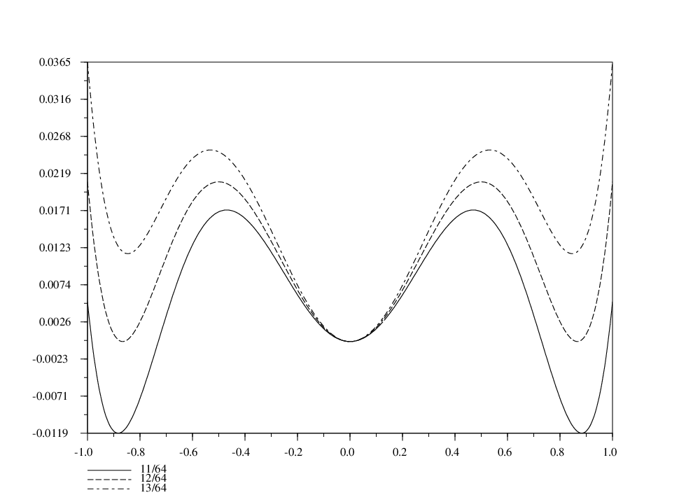
Refer to caption
Figure 2. The graph of Φ\Phi for m=11/64,m=12/64,m=13/64m=11/64,m=12/64,m=13/64.

In order to have a non trivial solution of (2.3) which tends to 00 at ±∞\pm\infty, we must choose mm so that Φ\Phi can vanish for non zero values of rr; letting

Ψ⁡(X)=m−X2+X23=X−1​Φ​(X),\Psi(X)=m-\frac{X}{2}+\frac{X^{2}}{3}=X^{-1}\Phi(\sqrt{X}),

it is immediate that ψ\psi can vanish for positive values of XX if and only if

m<316.m<\frac{3}{16}.

Henceforth, we will write

m=316​(1−ν)⟺ν=1−16​m3.m=\frac{3}{16}(1-\nu)\Longleftrightarrow\nu=1-\frac{16m}{3}.

The level curves of (r,s)↦s2−Φ⁡(r)(r,s)\mapsto s^{2}-\Phi(r) are represented at Fig. 3; this figure shows that there exist exactly two homoclinic orbits of (2.3) through 0 for m<3/16m<3/16; on one of them, rr takes only positive values, and on the other one rr takes only negative values. Therefore, we choose the homoclinic orbit which is situated in the half plane r≥0r\geq 0. The solution rr is still defined only up to translation. When rr reaches a maximum at some point x0x_{0}, r′​(x0)=0r^{\prime}(x_{0})=0, and ψ⁡(r2​(x0))\psi(r^{2}(x_{0})) vanishes.Therefore,

(2.7) r2​(x0)=3​(1−ν)4.r^{2}(x_{0})=\frac{3(1-\sqrt{\nu})}{4}.

Since (2.3) is invariant by the reflexion x↦2​x0−xx\mapsto 2x_{0}-x, we can see that r⁡(x)=r⁡(2​x0−x)r(x)=r(2x_{0}-x); if uu has more than one maximum, it is periodic, which is possible only if uu vanishes identically. Therefore, rr has exactly one maximum.

Refer to caption Refer to caption

Refer to caption
Figure 3. The level lines of (r,s)↦s2−Φ⁡(r)(r,s)\mapsto s^{2}-\Phi(r) for m=11/64m=11/64, m=12/64m=12/64, m=13/64m=13/64.

If we choose the translation parameter so that rr attains its maximum at 00, then rr is even and positive over ℝ\mathbb{R}, which concludes the proof of the lemma. ∎

In what follows, the dependence of rr or R=r2R=r^{2} over ν\nu will be emphasized from time to time, in which case, we will write r⁡(x,ν)r(x,\nu) or R⁡(x,ν)R(x,\nu) instead of r⁡(x)r(x) or R⁡(x)R(x).

The value of RR can be found explicitly; it is equal to

R⁡(x)=34​1−ν1+ν​cosh⁡2​x.R(x)=\frac{3}{4}\frac{1-\nu}{1+\sqrt{\nu}\cosh 2x}.

If we draw a graph of the values of rr or RR for different values of ν\nu, we can observe that the ‘width’ of rr or RR increases logarithmically with 1/ν1/\nu; see 4.

Refer to caption
Figure 4. The graph of RR over the interval [−10,10][-10,10], for ν=10−p/12,0≤p≤5\nu=10^{-p}/12,0\leq p\leq 5.

In fact, as ν\nu decreases to 00 RR is very close to a two front solution, and the distance between these two fronts can be estimated very precisely. This important observation in stated and proved in next Lemma:

Lemma 2.2.

Let

(2.8) L=14​ln⁡4ν⟺ν=4​e−4​L,L=\frac{1}{4}\ln\frac{4}{\nu}\Longleftrightarrow\nu=4e^{-4L},

and

(2.9) R~​(x)=34​11+e2​x.\tilde{R}(x)=\frac{3}{4}\frac{1}{1+e^{2x}}.

Then, we have the estimates for all x∈ℝx\in\mathbb{R}

(2.10) |R⁡(x+L)−R~​(x)|≤ν​e−2​x.\displaystyle\left|R(x+L)-\tilde{R}(x)\right|\leq\nu e^{-2x}.
(2.11) |R′​(x+L)−R~′​(x)|≤O⁡(1)​ν​e−2​x.\displaystyle\left|R^{\prime}(x+L)-\tilde{R}^{\prime}(x)\right|\leq O(1)\nu e^{-2x}.

Moreover, r~=R~\tilde{r}=\sqrt{\tilde{R}} is a solution of the differential equations

(2.12) −316​r~′′+W~​r~=0-\frac{3}{16}\tilde{r}^{\prime\prime}+\tilde{W}\tilde{r}=0

where

(2.13) W~=316−R~+R~2,\tilde{W}=\frac{3}{16}-\tilde{R}+\tilde{R}^{2},

and

(2.14) r~′=−r~​(1−4​r~23).\tilde{r}^{\prime}=-\tilde{r}\left(1-\frac{4\tilde{r}^{2}}{3}\right).
Proof.

We infer from (2.9) the relation

(2.15) e−2​x=R~​(x)3/4−R~​(x);e^{-2x}=\frac{\tilde{R}(x)}{3/4-\tilde{R}(x)};

it is also immediate that R~\tilde{R} satisfies the ordinary differential equation

(2.16) R~′=−2​R~​(1−4​R~/3),\tilde{R}^{\prime}=-2\tilde{R}(1-4\tilde{R}/3),

which can also be found by passing to the limit as ν\nu tends to 00 in the differential equation satisfied by RR:

(2.17) R′=±2​R​ψ⁡(R)/m.R^{\prime}={\pm 2}R\sqrt{\psi(R)/m}.

The definition (2.8) of LL and a direct computation give

(2.18) R(⋅+L)=(1−ν)​R~​(1−4​R~/3)1−4​R~/3+4​ν​R~2/9,R(\cdot+L)=\frac{(1-\nu)\tilde{R}(1-4\tilde{R}/3)}{1-4\tilde{R}/3+4\nu\tilde{R}^{2}/9},

from which we infer the identity

(2.19) R(⋅+L)−R~=−ν​R~​(1−2​R~/3)21−4​R~/3+4​ν​R~2/9.R(\cdot+L)-\tilde{R}=-\frac{\nu\tilde{R}(1-2\tilde{R}/3)^{2}}{1-4\tilde{R}/3+4\nu\tilde{R}^{2}/9}.

Thanks to (2.15), we deduce immediately (2.10) from (2.19). If we differentiate (2.19) with respect to xx, we find

R′(⋅+L)−R~′=−νR~′[(−4/3+8νR~/9)R~​(1−2​R~/3)2(1−4​R~/3+4​ν​R~2/9)2−(1−8​R~/3+4​R~2/3CLOSE1−4​R~/3+4​ν​R~2/9].\begin{split}&R^{\prime}(\cdot+L)-\tilde{R}^{\prime}\\ &=-\nu\tilde{R}^{\prime}\left[(-4/3+8\nu\tilde{R}/9)\frac{\tilde{R}(1-2\tilde{R}/3)^{2}}{(1-4\tilde{R}/3+4\nu\tilde{R}^{2}/9)^{2}}-\frac{(1-8\tilde{R}/3+4\tilde{R}^{2}/3}{1-4\tilde{R}/3+4\nu\tilde{R}^{2}/9}\right].\end{split}

Then, with the help of (2.16) and (2.15), relation (2.11) is clear. By a passage to the limit as ν\nu tends to 00, or by a direct computation, we see that (2.12), (2.13) and (2.14) hold. As xx tends to +∞+\infty, R~\tilde{R} tends to 0 and VV tends to 3/163/16. ∎

The linearized operator around rr is an unbounded operator AA in L2​(ℝ)L^{2}(\mathbb{R}) defined by

D⁡(A)=H2​(ℝ),A​u=−m​u′′+V​u,V=m−3​r2+5​r4.D(A)=H^{2}(\mathbb{R}),\quad Au=-mu^{\prime\prime}+Vu,\quad V=m-3r^{2}+5r^{4}.

The spectral properties of AA are important for what follows:

Lemma 2.3.

The operator AA is self-adjoint; its continuous spectrum is included in the interval [m,+∞)[m,+\infty); the infimum of the spectrum of AA is a strictly negative number λ\lambda, to which corresponds an even strictly positive eigenfunction ss. The function r′r^{\prime} is an eigenfunction of AA corresponding to the eigenvalue 00. Both λ\lambda and 00 are simple eigenvalues.

Proof.

Clearly, AA is self-adjoint. We have

V⁡(±∞)=m>0;V(\pm\infty)=m>0;

The essential spectrum of AA is contained in [m,+∞)[m,+\infty) (see Kato, [28],Theorem 5.26), and the spectrum of AA is bounded from below by minx⁡V⁡(x)\min_{x}V(x); for all β>0\beta>0, the intersection of the spectrum of AA with (−∞,m−β](-\infty,m-\beta] contains only eigenvalues of finite multiplicity; since AA is a Schrödinger operator in one-dimensional space, these eigenvalues are all simple; moreover, since rr is even, VV is even, and the eigenfunctions of AA are even or odd; in particular, an eigenfunction corresponding to the lowest eigenvalue λ\lambda of AA does not change sign, thanks to the maximum principle; therefore, it is even, since such an eigenfunction cannot vanish together with its derivative.

Denote by ss an eigenfunction of AA corresponding to λ\lambda; this ss can be chosen so that

s⁡(x)>0,∀x∈ℝ.s(x)>0,\forall x\in\mathbb{R}.

Differentiating (2.3) with respect to xx, we obtain

A​r′=0.Ar^{\prime}=0.

It is clear that r′r^{\prime} belongs to L2​(ℝ)L^{2}(\mathbb{R}); therefore, it is an eigenvector of AA, corresponding to the eigenvalue 00. On the other hand, r′r^{\prime} is odd; therefore, we have proved that the infimum of the spectrum of AA is a strictly negative number, λ\lambda. ∎

We will obtain later much more precise information on the spectrum of AA; but this information is easier to obtain if we take into account the nonlinearities of our problem ; in particular, we will asymptotically describe the eigenfunction ss in terms of the derivative of rr with respect to ν\nu, a feature which is clearly specific to our nonlinear situation. Thus, we have to study the dependence with respect to ν\nu of a number of objects which appear in this section.

Lemma 2.4.
  1. (i)

    The function

    ]0,1[→H2​(ℝ)ν↦r⁡(x,ν)\begin{matrix}]0,1[&\to&H^{2}(\mathbb{R})\\ \nu&\mapsto&r(x,\nu)\end{matrix}

    is infinitely differentiable.

  2. (ii)

    The eigenvalue λ⁡(ν)\lambda(\nu) and the eigenprojection P⁡(ν)P(\nu) on ℝ​s​(ν)\mathbb{R}s(\nu) are infinitely differentiable, respectively with values in ℝ\mathbb{R} and in the space of continuous operators in L2​(ℝ)L^{2}(\mathbb{R}).

Proof.

(i) Denote by Heven2​(ℝ)H^{2}_{\textrm{even}}(\mathbb{R}) (resp. Leven2​(ℝ)L^{2}_{\text{even}}(\mathbb{R})) the subspace of even functions belonging to H2​(ℝ)H^{2}(\mathbb{R}) (resp. L2​(ℝ)L^{2}(\mathbb{R})). Define a mapping ff from Heven2​(ℝ)×(0,1)H^{2}_{\textrm{even}}(\mathbb{R})\times(0,1) to Leven2​(ℝ)L^{2}_{\textrm{even}}(\mathbb{R}) by

f⁡(v,ν)=−m​v′′+m​v−v3+v5.f(v,\nu)=-mv^{\prime\prime}+mv-v^{3}+v^{5}.

This mapping is of class C∞C^{\infty}, we have f⁡(r,ν)=0f(r,\nu)=0, and D1​f​(r,ν)=AD_{1}f(r,\nu)=A, which is an isomorphism from Heven2H^{2}_{\text{even}} to Leven2​(ℝ)L^{2}_{\text{even}}(\mathbb{R}). Therefore, the implicit function theorem applies, and rr is a C∞C^{\infty} function of ν\nu with values in Heven2​(ℝ)H^{2}_{\textrm{even}}(\mathbb{R}).

(ii)If we divide AA by 1−ν1-\nu we obtain a Schrödinger operator whose differential part is constant, and whose potential part depends in a C∞C^{\infty} fashion on ν\nu, according to part (i) of this proof; therefore, we can apply the results of Kato, [28] IV.3, which enable us to conclude. ∎

Define three new functions σ⁡(x,ν)\sigma(x,\nu) and σ2​(x,ν)\sigma_{2}(x,\nu) by

(2.20) S⁡(x,ν)\displaystyle S(x,\nu) =−4​ν​∂R∂ν=∂∂L​R​(x,4​e−4​L)\displaystyle=-4\nu\frac{\partial R}{\partial\nu}=\frac{\partial}{\partial L}R\bigl(x,4e^{-4L}\bigr)
σ⁡(x,ν)\displaystyle\sigma(x,\nu) =−4​ν​∂r⁡(x,ν)∂ν=∂∂L​r​(x,4​e−4​L),\displaystyle=-4\nu\frac{\partial r(x,\nu)}{\partial\nu}=\frac{\partial}{\partial L}r(x,4e^{-4L}),
σ2​(x,ν)\displaystyle\sigma_{2}(x,\nu) =−4​ν​∂σ⁡(x,ν)∂ν=∂2∂L2​r​(x,4​e−4​L).\displaystyle=-4\nu\frac{\partial\sigma(x,\nu)}{\partial\nu}=\frac{\partial^{2}}{\partial L^{2}}r(x,4e^{-4L}).

The following lemma states that S+RxS+R_{x}, σ+rx\sigma+r_{x} and σ2+2​σx+rx​x\sigma_{2}+2\sigma_{x}+r_{xx} are very close to 00; this is really a consequence of the non linearity; the benefit will be even greater when we will show below that σ\sigma is an excellent approximation of the eigenfunction of AA corresponding to its lowest eigenvalue.

Lemma 2.5.

We have the following estimates for all x∈ℝ+x\in\mathbb{R}^{+}, and all ν∈(0,1)\nu\in(0,1):

(2.21) |S⁡(x,ν)+Rx​(x,ν)R⁡(x,ν)|\displaystyle\left|\frac{S(x,\nu)+R_{x}(x,\nu)}{R(x,\nu)}\right| ≤O⁡(1)​ν1−4​R~​(x−L)/3,\displaystyle\leq\frac{O(1)\nu}{1-4\tilde{R}(x-L)/3},
(2.22) |σ⁡(x,ν)+∂r∂x​(x,ν)|\displaystyle\left|\sigma(x,\nu)+\frac{\partial r}{\partial x}(x,\nu)\right| ≤O⁡(1)​ν​e−x,\displaystyle\leq O(1)\sqrt{\nu}\,e^{-x},
and
(2.23) |σ2​(x,ν)+2​∂σ∂x​(x,ν)+∂2r∂x2​(x,ν)|\displaystyle\left|\sigma_{2}(x,\nu)+2\frac{\partial\sigma}{\partial x}(x,\nu)+\frac{\partial^{2}r}{\partial x^{2}}(x,\nu)\right| ≤O⁡(1)​ν​e−x,\displaystyle\leq O(1)\sqrt{\nu}\,e^{-x},
Proof.

The differentiation of (2.18) with respect to LL gives

1R(⋅+L,4e−4​L)1∂LR(⋅+L,4e−4​L)=−4​ν1−ν(1−2​R~/3)21−4​R~/3+4​ν​R~2/9,\frac{1}{R\bigl(\cdot+L,4e^{-4L}\bigr)}\frac{1}{\partial L}R\bigl(\cdot+L,4e^{-4L}\bigr)=-\frac{4\nu}{1-\nu}\frac{(1-2\tilde{R}/3)^{2}}{1-4\tilde{R}/3+4\nu\tilde{R}^{2}/9},

which implies immediately (2.21). An analogous computation implies

(2.24) ∂∂L​[r⁡(x+L,4​e−4​L)]=rx​(x+L,4​e−4​L)+σ⁡(x+L,4​e−4​L),\frac{\partial}{\partial L}\bigl[r(x+L,4e^{-4L})\bigr]=r_{x}(x+L,4e^{-4L})+\sigma(x+L,4e^{-4L}),

and

(2.25) ∂2∂L2​[r⁡(x+L,4​e−4​L)]=rx​x​(x+L,4​e−4​L)+2​σx​(x+L,4​e−4​L)+σ2​(x+L,4​e−4​L).\begin{split}\frac{\partial^{2}}{\partial L^{2}}\bigl[r(x+L,4e^{-4L})\bigr]&=r_{xx}(x+L,4e^{-4L})\\ &\quad+2\sigma_{x}(x+L,4e^{-4L})+\sigma_{2}(x+L,4e^{-4L}).\end{split}

Differentiating (2.18), we find

∂∂Lr(⋅+L,4e−4​L)=2​ν​r~​(1−4​R~/3)​(1−2​R~/3)2(1−4​R~/3+4​ν​R~2/9)2,\frac{\partial}{\partial L}r(\cdot+L,4e^{-4L})=\frac{2\nu\tilde{r}(1-4\tilde{R}/3)(1-2\tilde{R}/3)^{2}}{(1-4\tilde{R}/3+4\nu\tilde{R}^{2}/9)^{2}},

and

∂2∂L2r(⋅+L,4e−4​L)=−8​ν​r~​(1−4​R~/3)​(1−2​R~/3)2​(1−4​R~/3−4​ν​R~2/9)(1−4​R~/3+4​ν​R~2/9)3−4​ν2​r~​(1−4​R~/3)2​(1−2​R~/3)4(1−4​R~/3+4​ν​R~2/9)4.\begin{split}\frac{\partial^{2}}{\partial L^{2}}r(\cdot+L,4e^{-4L})&=-\frac{8\nu\tilde{r}(1-4\tilde{R}/3)(1-2\tilde{R}/3)^{2}(1-4\tilde{R}/3-4\nu\tilde{R}^{2}/9)}{(1-4\tilde{R}/3+4\nu\tilde{R}^{2}/9)^{3}}\\ &-\frac{4\nu^{2}\tilde{r}(1-4\tilde{R}/3)^{2}(1-2\tilde{R}/3)^{4}}{(1-4\tilde{R}/3+4\nu\tilde{R}^{2}/9)^{4}}.\end{split}

Observe that

ν​r~1−4​R~/3=ν​34​e−x​(1+e−2​x)1/2,\frac{\nu\tilde{r}}{1-4\tilde{R}/3}=\nu\sqrt{\frac{3}{4}}e^{-x}\bigl(1+e^{-2x}\bigr)^{1/2},

so that:

(2.26) ∀x≥−L,ν​r~1−4​R~/3≤O⁡(1)​ν​e−x−L;\forall x\geq-L,\quad\frac{\nu\tilde{r}}{1-4\tilde{R}/3}\leq O(1)\sqrt{\nu}e^{-x-L};

moreover we have also

(2.27) ∀x≥−L,ν1−4​R~/3≤O⁡(1);\forall x\geq-L,\quad\frac{\nu}{1-4\tilde{R}/3}\leq O(1);

We use the information given by (2.26) and (2.27), to infer that

∀x≥−L,|∂∂Lr(⋅+L,4e−4​L)|≤O(1)νe−x−L,|∂2∂L2r(⋅+L,4e−4​L)|≤O(1)νe−x−L;\begin{split}\forall x\geq-L,\quad&\left|\frac{\partial}{\partial L}r(\cdot+L,4e^{-4L})\right|\leq O(1)\sqrt{\nu}e^{-x-L},\\ &\left|\frac{\partial^{2}}{\partial L^{2}}r(\cdot+L,4e^{-4L})\right|\leq O(1)\sqrt{\nu}e^{-x-L};\end{split}

the conclusion of the lemma follows immediately. ∎

For later purposes, we define

S⁡(x+L,4​e−4​L)=∂∂L​R​(x+L,4​e−4​L).S(x+L,4e^{-4L})=\frac{\partial}{\partial L}R(x+L,4e^{-4L}).

From here, we will obtain an upper estimate for the lower bound of the spectrum of AA:

Lemma 2.6.

We have

(A​σ,σ)(σ,σ)∼−3​ν2.\frac{(A\sigma,\sigma)}{(\sigma,\sigma)}\sim-\frac{3\nu}{2}.
Proof.

Let us compute A​σA\sigma by differentiating the equation

−m​r′′+m​r−r3+r5=0-mr^{\prime\prime}+mr-r^{3}+r^{5}=0

with respect to LL; we obtain

(2.28) A​σ=ρA\sigma=\rho

where

(2.29) ρ=4​ν1−ν​(r5−r3).\rho=\frac{4\nu}{1-\nu}(r^{5}-r^{3}).

To prove our assertion, we will have to calculate (σ,σ)(\sigma,\sigma) and (σ,ρ)(\sigma,\rho). From Lemma 2.5, we can see that

∫σ2​(x,ν)​𝑑x=2​∫0∞rx​(x,ν)2​𝑑x+O⁡(ν),\int\sigma^{2}(x,\nu)\,dx=2\int_{0}^{\infty}r_{x}(x,\nu)^{2}\,dx+O(\sqrt{\nu}),

and from estimate (2.11), we have

2​∫0∞rx​(x,ν)2​𝑑x=2​∫−L∞r~′​(x)2​𝑑x+O⁡(ν);2\int_{0}^{\infty}r_{x}(x,\nu)^{2}\,dx=2\int_{-L}^{\infty}\tilde{r}^{\prime}(x)^{2}\,dx+O(\sqrt{\nu});

but relations (2.14) and (2.16) imply that

|r~′|2=−12​R~′​(1−4​R~3);\left|\tilde{r}^{\prime}\right|^{2}=-\frac{1}{2}\tilde{R}^{\prime}\left(1-\frac{4\tilde{R}}{3}\right);

we infer from relation (2.7) that

(2.30) 2​∫−L∞|r~′|2​𝑑x=38+O⁡(ν),2\int_{-L}^{\infty}\left|\tilde{r}^{\prime}\right|^{2}\,dx=\frac{3}{8}+O\bigl(\sqrt{\nu}\bigr),

so that

(2.31) (σ,σ)=38+O⁡(ν).(\sigma,\sigma)=\frac{3}{8}+O(\sqrt{\nu}).

On the other hand,

(2.32) (r5−r3,σ)=−2∫0∞(r5−r3)rxdx+O(ν)=2​(R​(0,ν)36−R​(0,ν)24)+O⁡(ν)=−964+O⁡(ν).\begin{split}(r^{5}-r^{3},\sigma)&=-2\int_{0}^{\infty}(r^{5}-r^{3})r_{x}\,dx+O(\sqrt{\nu})\\ &=2\left(\frac{R(0,\nu)^{3}}{6}-\frac{R(0,\nu)^{2}}{4}\right)+O(\sqrt{\nu})\\ &=-\frac{9}{64}+O(\sqrt{\nu}).\end{split}

Thus, we obtain from (2.29) and (2.32) the relation

(2.33) (A​σ,σ)=−9​ν16+O⁡(ν3/2).(A\sigma,\sigma)=-\frac{9\nu}{16}+O(\nu^{3/2}).

The conclusion of the lemma is a direct consequence of (2.31) and (2.33). ∎

Theorem 2.7.

There exists a constant KK such that for all small enough ν\nu the spectrum of AA is partitioned in its intersection with the interval [−K,K][-K,K] and its intersection with interval [2K,+∞)[2K,+\infty).

Proof.

Define

V~​(x)=316−3​R~+5​R~2.\tilde{V}(x)=\frac{3}{16}-3\tilde{R}+5\tilde{R}^{2}.

It is clear that r~′\tilde{r}^{\prime} satisfies the Schrödinger equation

−r~′′′+V~​r~′=0.-\tilde{r}^{\prime\prime\prime}+\tilde{V}\tilde{r}^{\prime}=0.

As r~′\tilde{r}^{\prime} is strictly negative for all xx, this means that 00 is the lower bound of the spectrum of the operator A~\tilde{A} defined by

D⁡(A~)=H2​(ℝ),A~​v=−v′′+V~​v.D(\tilde{A})=H^{2}(\mathbb{R}),\tilde{A}v=-v^{\prime\prime}+\tilde{V}v.

As V~​(−∞)=3/4\tilde{V}(-\infty)=3/4 and V~​(+∞)=3/16\tilde{V}(+\infty)=3/16, the essential spectrum of A~\tilde{A} is included in [3/16,+∞)[3/16,+\infty), and thus the second eigenvalue of A~\tilde{A} is some number Λ>0\Lambda>0.

We use now the twisting trick of E. B. Davies [6]: define the operators

𝒥~=(−∂2+V~(⋅−L)00−∂2+V~(−⋅−L)),𝒥=(−∂2+3/400A);\tilde{\mathcal{J}}=\begin{pmatrix}-\partial^{2}+\tilde{V}(\cdot-L)&0\\ 0&-\partial^{2}+\tilde{V}(-\cdot-L)\end{pmatrix},\quad\mathcal{J}=\begin{pmatrix}-\partial^{2}+3/4&0\\ 0&A\end{pmatrix};

let η\eta be an infinitely differentiable function from ℝ\mathbb{R} to [0,π/2][0,\pi/2] which vanishes for x≤−1x\leq-1 and is equal to π/2\pi/2 for x≥1x\geq 1 and let ηL=η(⋅/L)\eta_{L}=\eta(\cdot/L). Define now a unitary transformation in L2​(ℝ)2L^{2}(\mathbb{R})^{2} by its matrix

UL=(cos⁡ηL−sin⁡ηLsin⁡ηLcos⁡ηL).U_{L}=\begin{pmatrix}\cos\eta_{L}&-\sin\eta_{L}\\ \sin\eta_{L}&\cos\eta_{L}\end{pmatrix}.

We compute UL​𝒥​UL∗U_{L}\mathcal{J}U_{L}^{*} and we find that

UL​∂2∂x2​UL∗=∂2∂x2+−η′(⋅/L)L​(0−110)​∂∂x−η′′(⋅/L)L2​(0−110)−(η′(⋅/L))2L2andUL​(V003/4)​UL∗=(V​cos2⁡ηL+(3​sin2⁡ηL)/4(cosηLsinηL)(V−3/4)(cosηLsinηL)(V−3/4)V​sin2⁡ηL+(3​cos2⁡ηL)/4).\begin{split}&U_{L}\frac{\partial^{2}}{\partial x^{2}}U_{L}^{*}=\frac{\partial^{2}}{\partial x^{2}}+-\frac{\eta^{\prime}(\cdot/L)}{L}\begin{pmatrix}0&-1\\ 1&0\end{pmatrix}\frac{\partial}{\partial x}-\frac{\eta^{\prime\prime}(\cdot/L)}{L^{2}}\begin{pmatrix}0&-1\\ 1&0\end{pmatrix}-\frac{\bigl(\eta^{\prime}(\cdot/L)\bigr)^{2}}{L^{2}}\\ \intertext{and}&U_{L}\begin{pmatrix}V&0\\ 0&3/4\end{pmatrix}U_{L}^{*}=\begin{pmatrix}V\cos^{2}\eta_{L}+\bigl(3\sin^{2}\eta_{L}\bigr)/4&\bigl(\cos\eta_{L}\sin\eta_{L}\bigl)(V-3/4)\\ \bigl(\cos\eta_{L}\sin\eta_{L}\bigr)(V-3/4)&V\sin^{2}\eta_{L}+\bigl(3\cos^{2}\eta_{L}\bigr)/4\end{pmatrix}.\end{split}

An elementary calculation shows now that

UL​𝒥​UL∗=𝒥~+BL​∂∂x+CLU_{L}\mathcal{J}U_{L}^{*}=\tilde{\mathcal{J}}+B_{L}\frac{\partial}{\partial x}+C_{L}

where BLB_{L} and CLC_{L} are matrix valued functions whose norm tends to 00 as LL tends to infinity. It is plain that the resolvent sets of 𝒥~\tilde{\mathcal{J}} and A~\tilde{A} are identical.

If EE and FF are Banach spaces, ℒ⁡(E,F)\mathcal{L}(E,F) is the space of linear bounded operators from EE to FF and ‖‖ℒ⁡(E,F)\left\|\>\>\right\|_{\mathcal{L}(E,F)} the corresponding norm; if E=FE=F, we abbreviate ℒ⁡(E,F)\mathcal{L}(E,F) to ℒ⁡(E)\mathcal{L}(E). If EE is the space L2​(ℝ)nL^{2}(\mathbb{R})^{n} we abbreviate ℒ⁡(E)\mathcal{L}(E) to ℒ\mathcal{L}.

Let zz belong to the resolvent set of A~\tilde{A}; then for every gg in L2​(ℝ)2L^{2}(\mathbb{R})^{2}, (𝒥~−z)−1(\tilde{\mathcal{J}}-z)^{-1} belongs to H2​(ℝ)2H^{2}(\mathbb{R})^{2}, and the function z↦∥(∂2/∂x2)(𝒥~−z)−1∥ℒ⁡(L2)z\mapsto\lVert(\partial^{2}/\partial x^{2})(\tilde{\mathcal{J}}-z)^{-1}\rVert_{{\mathcal{L}(L^{2})}} is continuous on the resolvent set of 𝒥~\tilde{\mathcal{J}}.

It is equivalent to solve

(𝒥~+BL​∂∂x+CL−z)​u=f\left(\tilde{\mathcal{J}}+B_{L}\frac{\partial}{\partial x}+C_{L}-z\right)u=f

and

g+(BL​∂∂x+CL)​(𝒥~−z)−1​g=f;g+\left(B_{L}\frac{\partial}{\partial x}+C_{L}\right)(\tilde{\mathcal{J}}-z)^{-1}g=f;

the previous considerations show that for all zz in the resolvent set of 𝒥~\tilde{\mathcal{J}}, we can find L⁡(z)L(z) such that for all L≥L⁡(z)L\geq L(z), zz is also in the resolvent set of 𝒥\mathcal{J}. In particular, if we take K=Λ/3K=\Lambda/3, we can find L¯\bar{L} such that for all L≥L¯L\geq\bar{L}, the segment (K,2​K)(K,2K) is included in the resolvent set of 𝒥\mathcal{J}. In particular, we see also that for all L≥L¯L\geq\bar{L}, the generalized eigenspace of AA relative to the interval [−min⁡V,K][-\min V,K] contains exactly two eigenvalues; the minimum of VV is equal to −21/80+O(ν)-21/80+O(\nu); the above considerations show that these two eigenvalues tend to 00 as ν\nu tends to 00. ∎

Let us prove now that λ\lambda is very close to (A​σ,σ)/(σ,σ)(A\sigma,\sigma)/(\sigma,\sigma).

Denote by Π\Pi the projection onto the sum of the eigenspaces relative to 00 and λ\lambda. We have

(2.34) Π=12​π​i​∫γ(ζ−A)−1​𝑑ζ,\Pi=\frac{1}{2\pi i}\int_{\gamma}(\zeta-A)^{-1}\,d\zeta,

where γ\gamma is a circle of radius 3​K/23K/2, which is traveled once in the positive direction.

Theorem 2.8.

We have the following estimates:

(2.35) |σ−Π​σ|H2​(ℝ)=O⁡(ν​L),|\sigma-\Pi\sigma|_{H^{2}(\mathbb{R})}=O(\nu\sqrt{L}),

and

(2.36) λ=−3​ν2+O⁡(ν3/2).\lambda=-\frac{3\nu}{2}+O\bigl(\nu^{3/2}\bigr).

In particular, we can choose s=Π​σs=\Pi\sigma as an eigenvector of AA relative to the eigenvalue λ\lambda, as soon as ν\nu is small enough. Moreover, if σ^\hat{\sigma} is the unique solution of

(2.37) Π​σ^=0,A​σ^=(𝟏−Π)​(λ​σ−ρ)\Pi\hat{\sigma}=0,\quad A\hat{\sigma}=(\boldsymbol{1}-\Pi)(\lambda\sigma-\rho)

then

(2.38) |Π​σ−σ−σ^|H2​(ℝ)=O⁡(ν2​L).\left|\Pi\sigma-\sigma-\hat{\sigma}\right|_{H^{2}(\mathbb{R})}=O\bigl(\nu^{2}\sqrt{L}\,\bigr).
Proof.

We observe that for |ζ|=3​K/2|\zeta|=3K/2, ζ−A\zeta-A is an isomorphism from H2​(ℝ)H^{2}(\mathbb{R}) to L2​(ℝ)L^{2}(\mathbb{R}) which transforms even functions into even functions, and odd functions into odd functions. Therefore, since σ\sigma is even by construction, Π​σ\Pi\sigma is even too.

We rewrite the identity A​σ=ρA\sigma=\rho as

σ=ρζ+(ζ−A)​σζ.\sigma=\frac{\rho}{\zeta}+\frac{(\zeta-A)\sigma}{\zeta}.

Hence, by integration along γ\gamma,

(2.39) Π​σ=σ+12​π​i​∫γ(ζ−A)−1​ζ−1​ρ​𝑑ζ.\Pi\sigma=\sigma+\frac{1}{2\pi i}\int_{\gamma}(\zeta-A)^{-1}\zeta^{-1}\rho\,d\zeta.

Since |ρ|=O⁡(ν​L)|\rho|=O(\nu\sqrt{L}), we obtain

(2.40) |σ−Π​σ|=O⁡(ν​L),|\sigma-\Pi\sigma|=O(\nu\sqrt{L}),

If ν\nu is small enough, (2.40) implies that Π​σ\Pi\sigma does not vanish identically. Thus, by construction it is an eigenfunction of AA relative to the eigenvalue 00 or to the eigenvalue λ\lambda. But we know that Π​σ\Pi\sigma is even; thus, it has to be an eigenfunction of AA relative to λ\lambda, and

λ=(A​Π​σ,Π​σ)(Π​σ,Π​σ).\lambda=\frac{(A\Pi\sigma,\Pi\sigma)}{(\Pi\sigma,\Pi\sigma)}.

But

(A​Π​σ,Π​σ)=(ρ,Π​σ)=(ρ,σ)+(ρ,Π​σ−σ)=(ρ,σ)+O⁡(L​ν2).(A\Pi\sigma,\Pi\sigma)=(\rho,\Pi\sigma)=(\rho,\sigma)+(\rho,\Pi\sigma-\sigma)=(\rho,\sigma)+O(L\nu^{2}).

and, on the other hand

(Π​σ,Π​σ)=(σ,Π​σ)=(σ,σ)+(Π​σ−σ,σ)=(σ,σ)+O⁡(ν​L).(\Pi\sigma,\Pi\sigma)=(\sigma,\Pi\sigma)=(\sigma,\sigma)+(\Pi\sigma-\sigma,\sigma)=(\sigma,\sigma)+O(\nu\sqrt{L}).

This proves (2.36).

In order to obtain (2.35) which holds in H2H^{2} norm, while (2.35) holds in L2L^{2} norm, we subtract the relation A​Π​σ=λ​Π​σA\Pi\sigma=\lambda\Pi\sigma from the relation A​σ=ρA\sigma=\rho and we obtain

m​|σx​x−(Π​σ)x​x|=|ρ−λ​Π​σ−V⁡(σ−Π​σ)|=O⁡(ν​L).m\bigl|\sigma_{xx}-(\Pi\sigma)_{xx}\bigr|=\bigl|\rho-\lambda\Pi\sigma-V(\sigma-\Pi\sigma)\bigr|=O(\nu\sqrt{L}).

For the last assertion of the theorem, we remark thanks to Cauchy’s theorem, the last term in (2.39) can be rewritten as

12​π​i​∫γ(ζ−A)−1​ζ−1​ρ​𝑑ζ=12​i​π​∫γ(ζ−A)−1​ζ−1​(𝟏−Π)​ρ​𝑑ζ=σ~\frac{1}{2\pi i}\int_{\gamma}(\zeta-A)^{-1}\zeta^{-1}\rho\,d\zeta=\frac{1}{2i\pi}\int_{\gamma}(\zeta-A)^{-1}\zeta^{-1}(\boldsymbol{1}-\Pi)\rho\,d\zeta=\tilde{\sigma}

and σ~\tilde{\sigma} is the unique solution of

(2.41) Π​σ~=0,A​σ~=(𝟏−Π)​ρ.\Pi\tilde{\sigma}=0,\quad A\tilde{\sigma}=(\boldsymbol{1}-\Pi)\rho.

Subtracting (2.41) from (2.37), we find that

Π⁡(σ~−σ^)=0,A⁡(σ~−σ^)=λ⁡(σ−Π​σ).\Pi(\tilde{\sigma}-\hat{\sigma})=0,\quad A(\tilde{\sigma}-\hat{\sigma})=\lambda\bigl(\sigma-\Pi\sigma).

and this implies immediately estimate (2.38), which concludes the proof. ∎

We need also the equation satisfied by σ2\sigma_{2}. If we differentiate (2.28) with respect to LL, we obtain

(2.42) A​σ2+(20​r3−6​r)​σ2=ρ2,A\sigma_{2}+(20r^{3}-6r)\sigma^{2}=\rho_{2},

where

ρ2=−4​ν​∂ρ∂ν+3​ν4​(σ′′−σ)=−16​ν(1−ν)2​(r5−r3)+8​ν1−ν​(5​r4−3​r2)​σ.\rho_{2}=-4\nu\frac{\partial\rho}{\partial\nu}+\frac{3\nu}{4}(\sigma^{\prime\prime}-\sigma)=-\frac{16\nu}{(1-\nu)^{2}}(r^{5}-r^{3})+\frac{8\nu}{1-\nu}(5r^{4}-3r^{2})\sigma.

Therefore,

(2.43) |ρ2|=O⁡(L​ν).|\rho_{2}|=O\bigl(\sqrt{L}\,\nu\bigr).

Moreover an analogous and straightforward argument shows that

(2.44) ∂λ∂L=0​(ν),|∂s∂L−σ2|=O⁡(L​ν).\frac{\partial\lambda}{\partial L}=0(\nu),\quad\left|\frac{\partial s}{\partial L}-\sigma_{2}\right|=O\bigl(\sqrt{L}\,\nu\bigr).

The final information we obtain are asymptotics on ∂λ/∂L\partial\lambda/\partial L on ∂s/∂L\partial s/\partial L:

Lemma 2.9.

The following estimates hold:

(2.45) ∂λ∂L=6​ν+O⁡(ν3/2),\displaystyle\frac{\partial\lambda}{\partial L}=6\nu+O\bigl(\nu^{3/2}\bigr),
(2.46) |∂s∂L−σ2|H2​(ℝ)=O⁡(ν​L).\displaystyle\left|\frac{\partial s}{\partial L}-\sigma_{2}\right|_{H^{2}(\mathbb{R})}=O\bigl(\nu\sqrt{L}\,\bigr).
Proof.

For the first estimate, we differentiate the relation

A​Π​σ=λ​Π​σA\Pi\sigma=\lambda\Pi\sigma

with respect to LL; we multiply scalarly the result

∂A∂L​Π​σ+A​∂Π​σ∂L=∂λ∂L​Π​σ+λ​∂Π​σ∂L\frac{\partial A}{\partial L}\Pi\sigma+A\frac{\partial\Pi\sigma}{\partial L}=\frac{\partial\lambda}{\partial L}\Pi\sigma+\lambda\frac{\partial\Pi\sigma}{\partial L}

by Π​σ\Pi\sigma and we obtain

|Π​σ|2​∂Π​σ∂L=(∂A∂L​Π​σ,Π​σ).\left|\Pi\sigma\right|^{2}\frac{\partial\Pi\sigma}{\partial L}=\left(\frac{\partial A}{\partial L}\Pi\sigma,\Pi\sigma\right).

Since

(2.47) ∂A∂L=4​ν1−ν​(A−3​r2+5​r4)−6​r​σ+20​r2​σ,\frac{\partial A}{\partial L}=\frac{4\nu}{1-\nu}\bigl(A-3r^{2}+5r^{4}\bigr)-6r\sigma+20r^{2}\sigma,

we may write

(∂A∂L​Π​σ,Π​σ)=4​ν​((3​r2−r4)​σ,σ)+((20​r3−6​r)​σ2,σ+2​σ^)+O⁡(ν2​L).\left(\frac{\partial A}{\partial L}\Pi\sigma,\Pi\sigma\right)=4\nu\bigl((3r^{2}-r^{4})\sigma,\sigma\bigr)+\bigl((20r^{3}-6r)\sigma^{2},\sigma+2\hat{\sigma}\bigr)+O(\nu^{2}L).

Thanks to (2.42),

((20​r3−6​r)​σ2,σ+2​σ^)=(A​σ2−ρ2,σ)=(σ2,ρ)−(ρ2,σ)+(σ2,λ​σ−ρ)+O⁡(ν3/2);\begin{split}&\bigl((20r^{3}-6r)\sigma^{2},\sigma+2\hat{\sigma}\bigr)=\bigl(A\sigma_{2}-\rho_{2},\sigma\bigr)\\ &\quad=(\sigma_{2},\rho)-(\rho_{2},\sigma)+(\sigma_{2},\lambda\sigma-\rho)+O\bigl(\nu^{3/2}\bigr);\end{split}

here we have used (2.37) and (2.35). Therefore,

OPEN(∂A∂L​Π​σ,Π​σ)=4​ν​((3​r2−r4)​σ,σ)+2​λ​σ2,σ)−∂∂L​(ρ,σ)+O⁡(ν3/2).\left(\frac{\partial A}{\partial L}\Pi\sigma,\Pi\sigma\right)=4\nu\bigl((3r^{2}-r^{4})\sigma,\sigma\bigr)+2\lambda\sigma_{2},\sigma)-\frac{\partial}{\partial L}(\rho,\sigma)+O(\nu^{3/2}).

At this point it is clear that there exists a number cc such that

(2.48) ∂λ∂L=c​ν+O⁡(ν3/2),\frac{\partial\lambda}{\partial L}=c\nu+O\bigl(\nu^{3/2}\bigr),

but the explicit calculation of cc is tedious. It can be avoided by integrating (2.48) with respect to LL: we see that

λ=−cν/4+O(ν3/2),\lambda=-c\nu/4+O\bigl(\nu^{3/2}\bigr),

and we infer from (2.36) that c=6c=6.

The other asymptotics are obtained as follows: we differentiate the relation

Π​σ=∫γ(ζ−A)−1​σ​𝑑σ\Pi\sigma=\int_{\gamma}(\zeta-A)^{-1}\sigma\,d\sigma

with respect to LL:

∂Π​σ∂L=12​i​π​∫γ(ζ−A)−1​[∂A∂L​(ζ−A)−1​σ+σ2]​𝑑ζ.\frac{\partial\Pi\sigma}{\partial L}=\frac{1}{2i\pi}\int_{\gamma}(\zeta-A)^{-1}\Bigl[\frac{\partial A}{\partial L}(\zeta-A)^{-1}\sigma+\sigma_{2}\Bigr]\,d\zeta.

We deduce from (2.38) that for ζ∈γ\zeta\in\gamma

|(ζ−A)−1​σ−(ζ−λ)−1|H2​(ℝ)=O⁡(ν​L);\left|(\zeta-A)^{-1}\sigma-(\zeta-\lambda)^{-1}\right|_{H^{2}(\mathbb{R})}=O\bigl(\nu\sqrt{L}\,\bigr);

therefore, it suffices to find an asymptotics for

12​i​π∫γ(ζ−A)−1(ζ−λ)−1[4​ν1−ν(ρ+(3r2−5r4)σ+ρ2−Aσ2+(ζ−λ)σ2]dζ.\frac{1}{2i\pi}\int\gamma(\zeta-A)^{-1}(\zeta-\lambda)^{-1}\Bigl[\frac{4\nu}{1-\nu}\bigl(\rho+(3r^{2}-5r^{4})\sigma+\rho_{2}-A\sigma_{2}+(\zeta-\lambda)\sigma_{2}\Bigr]\,d\zeta.

But

(ζ−A)−1​(ζ−λ)−1​(−A​σ2+(ζ−A)​σ2)=(ζ−λ)−1−λ​(ζ−A)−1​(ζ−λ)−1(\zeta-A)^{-1}(\zeta-\lambda)^{-1}\bigl(-A\sigma_{2}+(\zeta-A)\sigma_{2}\bigr)=(\zeta-\lambda)^{-1}-\lambda(\zeta-A)^{-1}(\zeta-\lambda)^{-1}

and it is clear now that (2.48) holds. ∎

3. The second equation

Let us first observe that we need only consider the case α>0\alpha>0: the mapping α↦−α\alpha\mapsto-\alpha transforms a solution into its conjugate.

There are two different ways of writing the full problem, each with a different scaling. The unscaled problem is

(3.1) −316​(1−ν)​u′′+316​(1−ν)​u−(1+i​α)​|u|2​u+|u|4​u+i​ω​u=0.-\frac{3}{16}(1-\nu)u^{\prime\prime}+\frac{3}{16}(1-\nu)u-(1+i\alpha)|u|^{2}u+|u|^{4}u+i\omega u=0.

Therefore, we define

F⁡(u,ω,α,ν)=−316​(1−ν)​u′′+316​(1−ν)​u−(1+i​α)​|u|2​u+|u|4​u+i​ω​u.F(u,\omega,\alpha,\nu)=-\frac{3}{16}(1-\nu)u^{\prime\prime}+\frac{3}{16}(1-\nu)u-(1+i\alpha)|u|^{2}u+|u|^{4}u+i\omega u.

Whenever necessary, we will use the components of uu, denoting them by u1u_{1} and u2u_{2}, so that u=u1+i​u2u=u_{1}+iu_{2}, and we define similarly the components of FF, F1F_{1} and F2F_{2}; therefore, we have

F=F1+i​F2.F=F_{1}+iF_{2}.

Let α=ε\alpha=\sqrt{\varepsilon}, u1=ξu_{1}=\xi, u2=η​εu_{2}=\eta\sqrt{\varepsilon}, ω=τ​ε\omega=\tau\sqrt{\varepsilon}. The scaled problem is

(3.2) G⁡(ξ,η,τ,ε,ν)=0,G(\xi,\eta,\tau,\varepsilon,\nu)=0,

where we define

(3.3) G⁡(ξ,η,τ,ε,ν)=F1​(ξ+i​ε​η,ε​τ,ε,ν)+iε​F2​(ξ+i​ε​η,ε​τ,ε,ν).G(\xi,\eta,\tau,\varepsilon,\nu)=F_{1}(\xi+i\sqrt{\varepsilon}\,\eta,\sqrt{\varepsilon}\tau,\sqrt{\varepsilon},\nu)+\frac{i}{{\sqrt{\varepsilon}}}F_{2}(\xi+i\sqrt{\varepsilon}\,\eta,\sqrt{\varepsilon}\tau,\sqrt{\varepsilon},\nu).

More explicitly,

G1​(ξ,η,τ,ε,ν)\displaystyle G_{1}(\xi,\eta,\tau,\varepsilon,\nu) =−τ​ε​η−316​(1−ν)​ξ′′+316​(1−ν)​ξ\displaystyle=-\tau\varepsilon\eta-\frac{3}{16}(1-\nu)\xi^{\prime\prime}+\frac{3}{16}(1-\nu)\xi
−(ξ−ε​η)​(ξ2+ε​η2)+(ξ2+ε​η2)2​ξ,\displaystyle\quad-(\xi-\varepsilon\eta)(\xi^{2}+\varepsilon\eta^{2})+(\xi^{2}+\varepsilon\eta^{2})^{2}\xi,
G2​(ξ,η,τ,ε,ν)\displaystyle G_{2}(\xi,\eta,\tau,\varepsilon,\nu) =τ​ξ−316​(1−ν)​η′′+316​(1−ν)​η\displaystyle=\tau\xi-\frac{3}{16}(1-\nu)\eta^{\prime\prime}+\frac{3}{16}(1-\nu)\eta
−(ξ+η)​(ξ2+ε​η2)+(ξ2+ε​η2)2​η.\displaystyle\quad-(\xi+\eta)(\xi^{2}+\varepsilon\eta^{2})+(\xi^{2}+\varepsilon\eta^{2})^{2}\eta.

Clearly, (3.2) is equivalent to (3.1). We will solve the existence problem looking at the GG formulation, and the stability problem looking at the FF formulation.

We have already determined a solution of

G1​(ξ,η,τ,0,ν)=0.G_{1}(\xi,\eta,\tau,0,\nu)=0.

it is given by ξ=r\xi=r, and η\eta and τ\tau are arbitrary.

In next lemma, we state the sense in which we can find a solution for the second equation at ε=0\varepsilon=0:

Lemma 3.1.

There exists a unique θ∈ℝ\theta\in\mathbb{R} and a unique qq in H2​(ℝ)H^{2}(\mathbb{R}) and orthogonal to rr which satisfy

(3.4) G2​(r,q,θ,0,ν)=0G_{2}(r,q,\theta,0,\nu)=0

Moreover, qq is even.

Proof.

The second equation at ε=0\varepsilon=0 can be written

τ​ξ−m​η′′+m​η−ξ3−ξ2​η+ξ4​η=0.\tau\xi-m\eta^{\prime\prime}+m\eta-\xi^{3}-\xi^{2}\eta+\xi^{4}\eta=0.

Therefore, if we let ξ=r\xi=r, we have to find qq and θ\theta such that (3.4) holds, i.e.

(3.5) B​q=−m​q′′+m​q−r2​q+r4​q=r3−θ​r.Bq=-mq^{\prime\prime}+mq-r^{2}q+r^{4}q=r^{3}-\theta r.

Define an unbounded operator BB in L2​(ℝ)L^{2}(\mathbb{R}) by

D⁡(B)=H2​(ℝ),B​u=−m​u′′+W​u,W=m−r2+r4.D(B)=H^{2}(\mathbb{R}),\quad Bu=-mu^{\prime\prime}+Wu,\quad W=m-r^{2}+r^{4}.

Clearly, BB is self adjoint. By construction

B​r=0.Br=0.

The lower bound of the essential spectrum of BB is m>0m>0; since rr is positive, the lower bound of the spectrum of BB is zero, which is a simple isolated eigenvalue. Therefore, solving (3.5) will be possible if and only if its right hand side r3−θ​rr^{3}-\theta r is orthogonal to ker⁡B=ℝ​r\ker B=\mathbb{R}r. This defines θ\theta thanks to

θ=∫r4​𝑑x∫r2​𝑑x.\theta=\frac{\int r^{4}\,dx}{\int r^{2}\,dx}.

Moreover, we define completely qq by requiring

(3.6) (q,r)=0.(q,r)=0.

It is clear that the qq we obtained belongs to H2​(ℝ)H^{2}(\mathbb{R}). Since the equation is invariant by the transformation x↦−xx\mapsto-x, qq has to be even. ∎

We will need precise asymptotic information, which we proceed to give now:

Lemma 3.2.

The number θ\theta is a C1C^{1} function of ν∈(0,1)\nu\in(0,1); we have the following asymptotics for θ\theta and ∂θ/∂L\partial\theta/\partial L:

(3.7) θ\displaystyle\theta =34−38​L+O⁡(ν).\displaystyle=\frac{3}{4}-\frac{3}{8L}+O(\sqrt{\nu}).
(3.8) θ1\displaystyle\theta_{1} =∂θ∂L=38​L2+O⁡(L−1​ν).\displaystyle=\frac{\partial\theta}{\partial L}=\frac{3}{8L^{2}}+O(L^{-1}\sqrt{\nu}).
Proof.

Let us compute the difference between 3/43/4 and θ\theta:

34−θ=∫0∞(3​r2/4−r4)​𝑑x∫0∞r2​𝑑x.\frac{3}{4}-\theta=\frac{\int_{0}^{\infty}(3r^{2}/4-r^{4})\,dx}{\int_{0}^{\infty}r^{2}\,dx}.

But an explicit computation and (2.10) give

∫0∞R​𝑑x=3​L4+38​ln⁡43+O⁡(ν),\int_{0}^{\infty}R\,dx=\frac{3L}{4}+\frac{3}{8}\ln\frac{4}{3}+O(\sqrt{\nu}),

that is

(3.9) ∫0∞R​𝑑x=3​L4+O⁡(ν).\int_{0}^{\infty}R\,dx=\frac{3L}{4}+O(\sqrt{\nu}).

In the same fashion,

∫0∞(3​R/4−R2)​𝑑x\displaystyle\int_{0}^{\infty}(3R/4-R^{2})\,dx =34​∫0∞R⁡(1−4​R/3)​𝑑x\displaystyle=\frac{3}{4}\int_{0}^{\infty}R(1-4R/3)\,dx
=34​∫0∞R~​(1−4​R~/3)​𝑑x+O⁡(ν)\displaystyle=\frac{3}{4}\int_{0}^{\infty}\tilde{R}(1-4\tilde{R}/3)\,dx+O(\sqrt{\nu})
=38​R~​(−L)+O⁡(ν)=932+O⁡(ν).\displaystyle=\frac{3}{8}\tilde{R}(-L)+O(\sqrt{\nu})=\frac{9}{32}+O(\sqrt{\nu}).

Therefore,

34−θ=38​L+O⁡(ν),\frac{3}{4}-\theta=\frac{3}{8L}+O(\sqrt{\nu}),

which implies immediately (3.7).

Since rr is a C∞C^{\infty} function of ν∈(0,1)\nu\in(0,1) with values in H2​(ℝ)H^{2}(\mathbb{R}), and it is integrable as well as σ\sigma, θ\theta is a C1C^{1} function of ν\nu. Let us compute ∂θ/∂L\partial\theta/\partial L; we have

(3.10) ∂θ∂L=(∫0∞r2​𝑑x​∫0∞4​r3​σ​𝑑x−∫0∞r4​𝑑x​∫0∞2​r​σ​𝑑x)​(∫0∞r2​𝑑x)−2.\frac{\partial\theta}{\partial L}=\left(\int_{0}^{\infty}r^{2}\,dx\int_{0}^{\infty}4r^{3}\sigma\,dx-\int_{0}^{\infty}r^{4}\,dx\int_{0}^{\infty}2r\sigma\,dx\right)\left(\int_{0}^{\infty}r^{2}\,dx\right)^{-2}.

But

∫0∞4r3σdx=−∫0∞4r3r′dx+O(ν)=R2(0)+O(ν)=916+O(ν).\int_{0}^{\infty}4r^{3}\sigma\,dx=-\int_{0}^{\infty}4r^{3}r^{\prime}\,dx+O(\sqrt{\nu})=R^{2}(0)+O(\sqrt{\nu})=\frac{9}{16}+O(\sqrt{\nu}).

Similarly,

∫0∞2rσdx=−∫0∞2rr′dx+O(ν)=R(0)+O(ν)=34+O(ν).\int_{0}^{\infty}2r\sigma\,dx=-\int_{0}^{\infty}2rr^{\prime}\,dx+O(\sqrt{\nu})=R(0)+O(\sqrt{\nu})=\frac{3}{4}+O(\sqrt{\nu}).

Therefore, the numerator of (3.10) is equal to

916​∫0∞R​dx−34​∫0∞R2​dx+O⁡(L​ν)=916​∫−L∞R~​(1−4​R~/3)​dx+O⁡(L​ν)=27128+O⁡(L​ν).\begin{split}&\frac{9}{16}\int_{0}^{\infty}R\,dx-\frac{3}{4}\int_{0}^{\infty}R^{2}\,dx+O(L\sqrt{\nu})=\frac{9}{16}\int_{-L}^{\infty}\tilde{R}(1-4\tilde{R}/3)\,dx+O(L\sqrt{\nu})\\ &=\frac{27}{128}+O(L\sqrt{\nu}).\end{split}

With the help of (3.9), we obtain  (3.8). ∎

Let us find now asymptotics for qq and related quantities. Let

(3.11) ϕ=qr.\phi=\frac{q}{r}.

Then ϕ\phi satisfies the ordinary differential equation:

−m⁡(ϕ′′​r+2​ϕ′​r′)=r3−θ​r.-m(\phi^{\prime\prime}r+2\phi^{\prime}r^{\prime})=r^{3}-\theta r.

Multiplying by rr we get

(3.12) m​(ϕ′​r2)′=θ​r2−r4.m(\phi^{\prime}r^{2})^{\prime}=\theta r^{2}-r^{4}.

Therefore,

m⁡(ϕ′​r2)​(x)=a+∫−∞x(θ​R−R2)​(y)​𝑑y.m(\phi^{\prime}r^{2})(x)=a+\int_{-\infty}^{x}(\theta R-R^{2})(y)\,dy.

But aa must vanish: q′q^{\prime} belongs to L2​(ℝ)L^{2}(\mathbb{R}) and is equal to ϕ​r′+ϕ′​r\phi r^{\prime}+\phi^{\prime}r; but

r′=−r​sgn⁡(x)​Ψ⁡(r)/m,r^{\prime}=-r\operatorname{sgn}(x)\sqrt{\Psi(r)/m},

hence

ϕ​r′=−q​sgn⁡(x)​Ψ⁡(r)/m,\phi r^{\prime}=-q\operatorname{sgn}(x)\sqrt{\Psi(r)/m},

so that ϕ′​r=q′−ϕ​r′\phi^{\prime}r=q^{\prime}-\phi r^{\prime} belongs to L2​(ℝ)L^{2}(\mathbb{R}). This implies that ϕ′​r2\phi^{\prime}r^{2} belongs to L2​(ℝ)L^{2}(\mathbb{R}) and hence aa vanishes. Therefore

(3.13) mϕ′(x)=1R⁡(x)∫−∞x(θ−R)Rdy=−1R⁡(x)∫x∞(θ−R)Rdy.m\phi^{\prime}(x)=\frac{1}{R(x)}\int_{-\infty}^{x}(\theta-R)R\,dy=-\frac{1}{R(x)}\int_{x}^{\infty}(\theta-R)R\,dy.
Lemma 3.3.

The following asymptotics hold for x≥0x\geq 0:

(3.14) ϕ′​(x)=−2−3​ln⁡(1−4​R~​(x−L)/3)4​L​R~​(x−L)+O⁡(ν/L).\displaystyle\phi^{\prime}(x)=-2-\frac{3\ln(1-4\tilde{R}(x-L)/3)}{4L\tilde{R}(x-L)}+O(\sqrt{\nu}/L).
(3.15) ϕ⁡(0)=L3+O⁡(1),\displaystyle\phi(0)=\frac{L}{3}+O(1),
(3.16) ϕ⁡(L)=−2​L3+O⁡(1)\displaystyle\phi(L)=-\frac{2L}{3}+O(1)
(3.17) |q|L1​(ℝ)=O⁡(L2),|q|L∞​(ℝ)=O⁡(L),|q|=O⁡(L3/2).\displaystyle|q|_{L^{1}(\mathbb{R})}=O(L^{2}),\quad|q|_{L^{\infty}(\mathbb{R})}=O(L),\quad|q|=O(L^{3/2}).
Proof.

From (3.13), we obtain

(3.18) mϕ′(x)=−1R⁡(x)(θ−3/4)∫x∞R(y)dy−1R⁡(x)∫x∞(3/4−R)Rdy.m\phi^{\prime}(x)=-\frac{1}{R(x)}(\theta-3/4)\int_{x}^{\infty}R(y)\,dy-\frac{1}{R(x)}\int_{x}^{\infty}(3/4-R)R\,dy.

For x>0x>0, we have thanks to (2.10)

∫x∞(3/4−R)​R​dy=∫x−L∞(3/4−R~)​R~​dy+O⁡(ν​e−2​x)=38​R~​(x−L)+O⁡(ν​e−2​x).\begin{split}&\int_{x}^{\infty}(3/4-R)R\,dy=\int_{x-L}^{\infty}(3/4-\tilde{R})\tilde{R}\,dy+O(\sqrt{\nu}e^{-2x})\\ &\quad=\frac{3}{8}\tilde{R}(x-L)+O(\sqrt{\nu}e^{-2x}).\end{split}

But relation (2.10) implies also that for x>0x>0

(3.19) |R⁡(x)R~​(x−L)−1|≤O⁡(1)​ν.\left|\frac{R(x)}{\tilde{R}(x-L)}-1\right|\leq O(1)\sqrt{\nu}\,.

Therefore,

(3.20) 1R⁡(x)​∫−∞x(3/4−R)​R​𝑑y=38+O⁡(ν).\frac{1}{R(x)}\int_{-\infty}^{x}(3/4-R)R\,dy=\frac{3}{8}+O(\sqrt{\nu}).

On the other hand,

∫x∞R​𝑑y=∫x−L∞R~​dy+ν​e−2​x​O​(1)=38​ln⁡(1+4​e2​L−2​x/3)+ν​O​(1)​4​R~​(x−L)1−4​R~​(x−L)/3.\begin{split}\int_{x}^{\infty}R\,dy&=\int_{x-L}^{\infty}\tilde{R}\,dy+\sqrt{\nu}\,e^{-2x}O(1)\\ &=\frac{3}{8}\ln\bigl(1+4e^{2L-2x}/3\bigr)+\nu O(1)\frac{4\tilde{R}(x-L)}{1-4\tilde{R}(x-L)/3}.\end{split}

Therefore, we have also

(3.21) 1R⁡(x)​∫x∞R​𝑑y=−38​ln⁡(1−4​R~​(x−L)/3)R~​(x−L)+O⁡(ν).\frac{1}{R(x)}\int_{x}^{\infty}R\,dy=-\frac{3}{8}\frac{\ln\bigl(1-4\tilde{R}(x-L)/3\bigr)}{\tilde{R}(x-L)}+O\bigl(\sqrt{\nu}\,\bigr).

Thus we have obtained the asymptotic for x≥0x\geq 0

(3.22) ∫x∞R⁡(θ−R)​𝑑y=R⁡(38−38​[θ−34]​ln⁡(1−4​R~​(x−L)/3)R~​(x−L)+O⁡(ν)).\int_{x}^{\infty}R(\theta-R)\,dy=R\left(\frac{3}{8}-\frac{3}{8}\left[\theta-\frac{3}{4}\right]\frac{\ln\bigl(1-4\tilde{R}(x-L)/3\bigr)}{\tilde{R}(x-L)}+O\bigl(\sqrt{\nu}\,\bigr)\right).

Relation (3.14) is an immediate consequence of (3.22).

In order to have an asymptotic for ϕ⁡(0)\phi(0), we will give another asymptotic for ϕ′\phi^{\prime}, which will be much less precise, but more usable at this level of the discussion; nevertheless, the precise asymptotic (3.14) will be useful later.

For x≥Lx\geq L,

ln⁡(1−4​R~​(x−L)/3)=−4​R~​(x−L)3+R~​(x−L)2​O​(1).\ln\bigl(1-4\tilde{R}(x-L)/3\bigr)=-\frac{4\tilde{R}(x-L)}{3}+\tilde{R}(x-L)^{2}O(1).

Therefore, for x≥Lx\geq L,

ϕ′​(x)=−2+1L+O⁡(1)​R~​(x−L)L+O⁡(ν).\phi^{\prime}(x)=-2+\frac{1}{L}+O(1)\frac{\tilde{R}(x-L)}{L}+O(\sqrt{\nu}).

In the same fashion, for 0≤x≤L0\leq x\leq L,

−ln⁡(1−4​R~​(x−L)/3)=ln⁡(1+e2​(L−x))=2​(L−x)+O⁡(1)​e2​(x−L)-\ln\bigl(1-4\tilde{R}(x-L)/3\bigr)=\ln\bigl(1+e^{2(L-x)}\bigr)=2(L-x)+O(1)e^{2(x-L)}
(3.23) ϕ′​(x)={−2x/L+O(1/L)e2​(x−L)if 0≤x≤L,−2+O⁡(1/L)if x≥L.\phi^{\prime}(x)=\begin{cases}-2x/L+O(1/L)e^{2(x-L)}&\text{if $0\leq x\leq L$,}\\ -2+O(1/L)&\text{if $x\geq L$.}\end{cases}

By integration in xx, we get now

(3.24) ϕ⁡(x)−ϕ⁡(0)={−x2/L+O(1),if 0≤x≤L,L−2​x+O⁡(1)+(x−L)​O​(1/L),if x≥L.\phi(x)-\phi(0)=\begin{cases}-x^{2}/L+O(1),&\text{if $0\leq x\leq L$,}\\ L-2x+O(1)+(x-L)O(1/L),&\text{if $x\geq L$.}\end{cases}

The value of ϕ⁡(0)\phi(0) is determined by the condition that qq should be orthogonal to rr (see Lemma 3.1). Therefore,

ϕ⁡(0)​∫0∞R⁡(x)​𝑑x\displaystyle\phi(0)\int_{0}^{\infty}R(x)\,dx =∫0L(x2L+O⁡(1))​R​(x)​𝑑x\displaystyle=\int_{0}^{L}\left(\frac{x^{2}}{L}+O(1)\right)R(x)\,dx
+∫L∞(−L+2x)R(x)dx+∫L∞(O(1)+x−LLO(1))R(x)dx.\displaystyle\quad+\int_{L}^{\infty}(-L+2x)R(x)\,dx+\int_{L}^{\infty}\biggl(O(1)+\frac{x-L}{L}O(1)\biggr)R(x)\,dx.

At this point we observe that

∫0∞R​𝑑x=3​L4+O⁡(1),∫0∞(x2/L+O⁡(1))​R​(x)​𝑑x=L24+O⁡(L),\displaystyle\int_{0}^{\infty}R\,dx=\frac{3L}{4}+O(1),\quad\int_{0}^{\infty}\bigl(x^{2}/L+O(1)\bigr)R(x)\,dx=\frac{L^{2}}{4}+O(L),
∫L∞(2​x−L)​R​(x)​𝑑x=O⁡(L),∫L∞(O⁡(1)+O⁡(1)​(x−L)/L)​R​(x)​𝑑x=O⁡(1).\displaystyle\int_{L}^{\infty}(2x-L)R(x)\,dx=O(L),\quad\int_{L}^{\infty}\bigl(O(1)+O(1)(x-L)/L\bigr)R(x)\,dx=O(1).

This yields the first relation in (3.15). The second relation in (3.16) is a consequence of the first together with (3.24).

Estimates (3.17) are a direct consequence of the definition  (3.11) of ϕ\phi, of the equivalents (3.23) and of (3.15) and (3.16). ∎

Since 00 is an isolated eigenvalue of BB for all ν\nu in (0,1)(0,1) and since (1−ν)−1​W(1-\nu)^{-1}W is an infinitely differentiable function of ν\nu with values in the space Cb2C^{2}_{b} of functions bounded as well as their first two derivatives in space, we can see that qq is a C∞C^{\infty} mapping from ν∈(0,1)\nu\in(0,1) to H2​(ℝ)H^{2}(\mathbb{R}), under the normalizing condition (3.6).

Differentiation of qq with respect to LL will be useful too; define

q1=∂∂L​q​(x,4​e−4​L).q_{1}=\frac{\partial}{\partial L}q(x,4e^{-4L}).

If we differentiate (3.5) with respect to LL we obtain

(3.25) B​q1+(4​r3−2​r)​q​σ=ρ^+3​r2​σ−θ​σ−θ1​r,Bq_{1}+(4r^{3}-2r)q\sigma=\hat{\rho}+3r^{2}\sigma-\theta\sigma-\theta_{1}r,

where

(3.26) ρ^=4​ν1−ν​(r4​q−r2​q−r3+θ​r).\hat{\rho}=\frac{4\nu}{1-\nu}(r^{4}q-r^{2}q-r^{3}+\theta r).

We recall that θ1\theta_{1} has been defined at (3.8)

We will need an estimate over ϕ′′\phi^{\prime\prime}. From (3.12), we have

m​ϕ′′=−R+θ−2​m​ϕ′​r′/r.m\phi^{\prime\prime}=-R+\theta-2m\phi^{\prime}r^{\prime}/r.

Assume that x≤0x\leq 0 and Write

a=ϕ′​(x)−22;a=\frac{\phi^{\prime}(x)-2}{2};

then, thanks to (2.17), we have

−2mϕ′r′/r=−2(1+a)mR′=−(1−ν)(1+a)(34−R+O(ν),-2m\phi^{\prime}r^{\prime}/r=-2(1+a)mR^{\prime}=-(1-\nu)(1+a)\left(\frac{3}{4}-R+O(\sqrt{\nu}\right),

so that

θ−R−−2​m​ϕ′​r′/r=θ−34−(34−R)​a+O⁡(ν).\theta-R--2m\phi^{\prime}r^{\prime}/r=\theta-\frac{3}{4}-\left(\frac{3}{4}-R\right)a+O\bigl(\sqrt{\nu}\bigr).

But the following expressions are bounded independently of ν\nu for x≤0x\leq 0:

(34−R~​(|x|−L))​ln⁡(1−4​R~​(|x|−L)/3)R~​(|x|−L)​ and ​ν​ex​ln⁡(1−4​R~​(|x|−L)/3)R~​(|x|−L);\left(\frac{3}{4}-\tilde{R}(\left|x\right|-L)\right)\frac{\ln(1-4\tilde{R}(\left|x\right|-L)/3)}{\tilde{R}(\left|x\right|-L)}\text{ and }\sqrt{\nu}e^{x}\frac{\ln(1-4\tilde{R}(\left|x\right|-L)/3)}{\tilde{R}(\left|x\right|-L)};

therefore, the term a⁡(3/4−R)a(3/4-R) is an O⁡(1/L)O(1/L), and we conclude with the help of (3.7) that

(3.27) |ϕ′′|∞=O⁡(L−1).|\phi^{\prime\prime}|_{\infty}=O(L^{-1}).

We will give now two estimates on the second lowest eigenvalue μ2\mu_{2} of BB; this eigenvalue is the lowest eigenvalue of BB restricted to odd functions.

Lemma 3.4.

The second lowest eigenvalue μ2\mu_{2} of BB satisfies

(3.28) μ2=m​π24​L2+O(L−5/2).\mu_{2}=\frac{m\pi^{2}}{4L^{2}}+O(L^{-5/2}).
Proof.

If t2t_{2} is an eigenvalue of BB, it is odd, thanks to the general Sturm-Liouville theory. Define an operator B0B_{0} in L2​(ℝ+)L^{2}(\mathbb{R}^{+}) by

D⁡(B0)=H01​(ℝ+)∩H2​(ℝ+),B0​u=B​u∣ℝ+;D(B_{0})=H^{1}_{0}(\mathbb{R}^{+})\cap H^{2}(\mathbb{R}^{+}),\quad B_{0}u=Bu\mid_{\mathbb{R}^{+}};

then μ2\mu_{2} is the first eigenvalue of B0B_{0}. In particular, for all v∈H01​(ℝ+)∖{0}v\in H^{1}_{0}(\mathbb{R}^{+})\setminus\{0\}, the following inequality holds:

μ2≤∫0∞(m​|v′|2+W​v2)​(∫0∞v2​𝑑x)−1.\mu_{2}\leq\int_{0}^{\infty}\bigl(m\left|v^{\prime}\right|^{2}+Wv^{2}\bigr)\left(\int_{0}^{\infty}v^{2}\,dx\right)^{-1}.

Define a test function vv by

v⁡(x)={sin⁡(π​x/2​(L−L))if 0≤x≤L−L,r⁡(x)/r⁡(L−L).if x≥L−L.v(x)=\begin{cases}\sin\bigl(\pi x/2\bigl(L-\sqrt{L}\bigr)\bigr)&\text{if $0\leq x\leq L-\sqrt{L}$,}\\ r(x)/r\bigl(L-\sqrt{L}\bigr).&\text{if $x\geq L-\sqrt{L}$.}\end{cases}

For all large enough LL, W≤0W\leq 0 on [0,L−L]\bigl[0,L-\sqrt{L}\bigr]; therefore an integration by parts on [L−L,+∞)\bigl[L-\sqrt{L},+\infty\bigr) shows that

∫0∞(m​|v′|2+W​v2)​𝑑x≤π2​m8​(L−L)3−R′​(L−L)R⁡(L−LCLOSE.\int_{0}^{\infty}\bigl(m\left|v^{\prime}\right|^{2}+Wv^{2}\bigr)\,dx\leq\frac{\pi^{2}m}{8\bigl(L-\sqrt{L}\bigr)^{3}}-\frac{R^{\prime}\bigl(L-\sqrt{L}\bigr)}{R(L-\sqrt{L}}.

On the other hand,

∫0L−Lv2​𝑑x≥L−L2;\int_{0}^{L-\sqrt{L}}v^{2}\,dx\geq\frac{L-\sqrt{L}}{2};

therefore, we see now that

(3.29) μ2≤π2m/8L2+O(L−5/2.\mu_{2}\leq\pi^{2}m/8L^{2}+O(L^{-5/2}.

Conversely, define L1>0L_{1}>0 by

R⁡(L1)=12​(1+1+3​ν+16​μ22);R(L_{1})=\frac{1}{2}\left(1+\frac{\sqrt{1+3\nu+16\mu_{2}}}{2}\right);

then, thanks to (2.10) and (3.29)

L1=L+12​ln⁡2+O⁡(1/L2);L_{1}=L+\frac{1}{2}\ln 2+O(1/L^{2});

the function x↦μ2−W⁡(x)x\mapsto\mu_{2}-W(x) changes sign only at x=L1x=L_{1}; therefore, there exists L2≤L1L_{2}\leq L_{1} such that t2t_{2} increases on [0,L2][0,L_{2}] and decreases on [L2,∞)[L_{2},\infty).

Case 1: L2≤L−LL_{2}\leq L-\sqrt{L}. Write M=μ2/mM=\sqrt{\mu_{2}/m}; since t2t_{2} and t2′t^{\prime}_{2} cannot vanish simultaneously and t2​(0)t_{2}(0) vanishes, there exists a continuous determination of the angle γ\gamma such that

(3.30) t2=b​sin⁡M​γ,t2′=b​M​cos⁡M​γ,γ⁡(0)=0.t_{2}=b\sin M\gamma,\quad t^{\prime}_{2}=bM\cos M\gamma,\quad\gamma(0)=0.

A classical calculation gives

1−γ′=Wm​M2​sin2⁡M​γ.1-\gamma^{\prime}=\frac{W}{mM^{2}}\sin^{2}M\gamma.

There exists a constant CC such that for all LL large enough,

∀x∈[0,L−L],0≤−W⁡(x)≤C​e−2​L;\forall x\in\bigl[0,L-\sqrt{L}\bigr],\quad 0\leq-W(x)\leq Ce^{-2\sqrt{L}};

if we let ε2=C​m​e−2​L\varepsilon^{2}=Cme^{-2\sqrt{L}}, γ\gamma satisfies the differential inequality by integration of the inequality

γ′≤1+ε​γ​(x)2,\gamma^{\prime}\leq 1+\varepsilon\gamma(x)^{2},

which we integrate as:

(3.31) γ⁡(x)≤ε−1​tan⁡(ε​x).\gamma(x)\leq\varepsilon^{-1}\tan\bigl(\varepsilon x).

Thanks to (3.30), M​γ​(L2)=π/2M\gamma(L_{2})=\pi/2; therefore thanks to (3.31),

M≥ε​π/2​tan⁡(ε​L2);M\geq\varepsilon\pi/2\tan(\varepsilon L_{2});

but the definition of ε\varepsilon and the condition on L2L_{2} imply immediately that

M≥π2​(1+C​ε2)​(L−L)M\geq\frac{\pi}{2(1+C\varepsilon^{2})\bigl(L-\sqrt{L}\bigr)}

which implies immediately the desired estimate (3.28).

Case 2: L2≥L−LL_{2}\geq L-\sqrt{L}. We have to give a different argument: multiply the equation −m​t2′′+W​t2=μ2​t2-mt_{2}^{\prime\prime}+Wt_{2}=\mu_{2}t_{2} by vv and perform two integration by parts on the term involving a second derivative; we eventually obtain

(m​π24​(L−L)2−μ2)∫0L−Lt2vdx=−∫0L−Lt2Wvdx+μ2∫L−L∞t2vdx+m​t2​(L−L)​[v′​(L−L−0)−v′​(L−L+0)].\begin{split}&\left(\frac{m\pi^{2}}{4\bigl(L-\sqrt{L}\bigr)^{2}}-\mu_{2}\right)\int_{0}^{L-\sqrt{L}}t_{2}v\,dx=-\int_{0}^{L-\sqrt{L}}t_{2}Wv\,dx+\mu_{2}\int_{L-\sqrt{L}}^{\infty}t_{2}v\,dx\\ &\qquad\qquad+mt_{2}(L-\sqrt{L})\bigl[v^{\prime}\bigl(L-\sqrt{L}-0\bigr)-v^{\prime}\bigl(L-\sqrt{L}+0\bigr)\bigr].\end{split}

Normalize t2t_{2} so that t2​(L2)=1t_{2}(L_{2})=1; then, by concavity on [0,L2][0,L_{2}],

t2​(x)≥x/L2≥x/L1;t_{2}(x)\geq x/L_{2}\geq x/L_{1};

therefore, there exists C>0C>0 such that

∫0L−Lt2​v​𝑑x≥C​L;\int_{0}^{L-\sqrt{L}}t_{2}v\,dx\geq CL;

on the other hand,

|∫0L−Lt2Wvdx|=O(Le−2​L),∫L−L∞t2vdx=O(L),|v′​(L−L−0)−v′​(L−L+0)|=O⁡(e−2​L)\begin{split}&\left|\int_{0}^{L-\sqrt{L}}t_{2}Wv\,dx\right|=O\bigl(Le^{-2\sqrt{L}}\bigr),\quad\int_{L-\sqrt{L}}^{\infty}t_{2}v\,dx=O\bigl(\sqrt{L}\bigr),\\ &\left|v^{\prime}\bigl(L-\sqrt{L}-0\bigr)-v^{\prime}\bigl(L-\sqrt{L}+0\bigr)\right|=O\bigl(e^{-2\sqrt{L}}\bigr)\end{split}

Therefore

CL|m​π24​(L−L)2−μ2|=O(L−3/2),CL\left|\frac{m\pi^{2}}{4\bigl(L-\sqrt{L}\bigr)^{2}}-\mu_{2}\right|=O\bigl(L^{-3/2}\bigr),

which implies immediately (3.29).

This proves Lemma 3.4. ∎

4. Existence of pulses

We will prove that there are couples (ξ,η)(\xi,\eta) which satisfy (3.2); the main idea is to use an ansatz suggested by previous long computations; this ansatz relies on the observation that for small values of ε\varepsilon, the pulse is simply stretched; i.e., the new pulse obtained should be very close to a pulse with ε=0\varepsilon=0 but a smaller value of ν\nu. In fact, we will work in reverse: given ν\nu, we define ν♭=ν​e−4​y\nu^{\flat}=\nu e^{-4y}, with y≥0y\geq 0; we let L♭=L+yL^{\flat}=L+y, r♭=r⁡(⋅,ν♭)r^{\flat}=r(\cdot,\nu^{\flat}), q♭=q⁡(⋅,ν♭)q^{\flat}=q(\cdot,\nu^{\flat}), θ♭=θ⁡(⋅,ν♭)\theta^{\flat}=\theta(\cdot,\nu^{\flat}), s♭=s⁡(⋅,ν♭)s^{\flat}=s(\cdot,\nu^{\flat}) and we have to determine an ansatz ε♭\varepsilon^{\flat} for ε\varepsilon. We will start with this ansatz, with very little motivation. The justification will be provided by the proofs which come later.

Once the ansatz is determined, we get an asymptotic description of the behavior of ε♭\varepsilon^{\flat}. Then, we go on to apply a version of the implicit function theorem cum estimates which is given in the appendix; for this purpose, we have to check that G⁡(r♭,q♭,θ♭,ε♭,ν)G(r^{\flat},q^{\flat},\theta^{\flat},\varepsilon^{\flat},\nu) is very small, that D(ξ,η,τ,ε)​G​(r♭,q♭,θ♭,ε♭,ν)D_{(\xi,\eta,\tau,\varepsilon)}G(r^{\flat},q^{\flat},\theta^{\flat},\varepsilon^{\flat},\nu) is invertible, with an estimate on the norm of its inverse; this necessitates an adequate choice of functional spaces; finally, we check that the second derivatives of GG are not too large in a neighborhood of (r♭,q♭,θ♭,ε♭)(r^{\flat},q^{\flat},\theta^{\flat},\varepsilon^{\flat}), and we are able to apply this implicit function theorem.

Moreover, we obtain precise asymptotics on the second term of the expansion. These estimates are crucial for the proof of the skew stabilization.

Define

(4.1) g1​(ε)=G1​(r♭,q♭,θ♭,ε,ν).g_{1}(\varepsilon)=G_{1}(r^{\flat},q^{\flat},\theta^{\flat},\varepsilon,\nu).

Another expression of g1g_{1} obtained by substituting the value of (−r′′+r)♭(-r^{\prime\prime}+r)^{\flat} from (2.3) is

(4.2) g1​(ε)=ν−ν♭1−ν♭​(r5−r3)♭+ε​(r2​q+2​r3​q2−r​q2−θ​q)♭+ε2​(r​q4+q3)♭.g_{1}(\varepsilon)=\frac{\nu-\nu^{\flat}}{1-\nu^{\flat}}(r^{5}-r^{3})^{\flat}+\varepsilon(r^{2}q+2r^{3}q^{2}-rq^{2}-\theta q)^{\flat}+\varepsilon^{2}(rq^{4}+q^{3})^{\flat}.

The ansatz for ε\varepsilon is given by

(4.3) (g1​(ε♭),s♭)=0.(g_{1}(\varepsilon^{\flat}),s^{\flat})=0.

Our purpose now is to show that this ansatz determines uniquely ε♭\varepsilon^{\flat} for small enough values of ν\nu, and for all y≥0y\geq 0. Let us introduce new notations

(4.4) κ\displaystyle\kappa =ν−ν♭1−ν♭,\displaystyle=\frac{\nu-\nu^{\flat}}{1-\nu^{\flat}},
a0\displaystyle a_{0} =(r5−r3,s),\displaystyle=(r^{5}-r^{3},s),
(4.5) a1\displaystyle a_{1} =(r2​q+2​r3​q2−r​q2−θ​q,s),\displaystyle=(r^{2}q+2r^{3}q^{2}-rq^{2}-\theta q,s),
a2\displaystyle a_{2} =(r​q4+q3,s).\displaystyle=(rq^{4}+q^{3},s).

Of course, aj♭a_{j}^{\flat} will be equal to aja_{j} with rr, qq, θ\theta and ss replaced by their analogues r♭r^{\flat}, q♭q^{\flat}, θ♭\theta^{\flat} and s♭s^{\flat}.

Therefore, (4.3) is equivalent to the following equation of the second degree:

(4.6) κ​a0♭+ε♭​a1♭+(ε♭)2​a2♭=0.\kappa a_{0}^{\flat}+\varepsilon^{\flat}a_{1}^{\flat}+(\varepsilon^{\flat})^{2}a_{2}^{\flat}=0.

In order to have an asymptotic for ε♭\varepsilon^{\flat} we will need an asymptotic for aja_{j}, 0≤j≤20\leq j\leq 2.

We introduce the notation

𝒪⁡(1)\mathcal{O}(1)

for any quantity whose absolute value or relevant norm is bounded by some power of LL.

Lemma 4.1.

The following asymptotics hold

(4.7) a0\displaystyle a_{0} =−964+O⁡(ν),\displaystyle=-\frac{9}{64}+O(\sqrt{\nu}),
(4.8) a1\displaystyle a_{1} =916+O⁡(1L),\displaystyle=\frac{9}{16}+O\left(\frac{1}{L}\right),
(4.9) a2\displaystyle a_{2} =L436+O⁡(L3).\displaystyle=\frac{L^{4}}{36}+O(L^{3}).
Proof.

We have

(r5−r3,s)=(r5−r3,σ)+O(νL)=−2∫0∞(r5−r3)r′dx+O(ν)=−964+O⁡(ν).\begin{split}(r^{5}-r^{3},s)&=(r^{5}-r^{3},\sigma)+O(\nu L)=-2\int_{0}^{\infty}(r^{5}-r^{3})r^{\prime}\,dx+O(\sqrt{\nu})\\ &=-\frac{9}{64}+O(\sqrt{\nu}).\end{split}

This gives (4.7).

The second object is more difficult. If we define

(4.10) a=(r2​q+2​r3​q2−r​q2−θ​q,σ)a=(r^{2}q+2r^{3}q^{2}-rq^{2}-\theta q,\sigma)

estimate (2.40) implies that |a1−a|=ν​𝒪​(1)\left|a_{1}-a\right|=\nu\mathcal{O}(1). But, thanks to (3.5) and (3.25), a~\tilde{a} can be rewritten as

a=((r2−θ)​q,σ)+12​(ρ^,q)+12​(3​r2​σ−θ​σ−θ1​r,q)−12​(q1,r3−B​r).a=\bigl((r^{2}-\theta)q,\sigma)+\frac{1}{2}(\hat{\rho},q)+\frac{1}{2}(3r^{2}\sigma-\theta\sigma-\theta_{1}r,q)-\frac{1}{2}(q_{1},r^{3}-Br).

Thus, we have

a=−(r4−θ​r2,ϕ1)+12​∂∂L​(r4−θ​r2,ϕ)+12​(ρ^,q).a=-(r^{4}-\theta r^{2},\phi_{1})+\frac{1}{2}\frac{\partial}{\partial L}(r^{4}-\theta r^{2},\phi)+\frac{1}{2}(\hat{\rho},q).

We transform this expression using (3.12):

(4.11) a=(m​(r2​ϕ′)′,ϕ1)−12​∂∂L​(m​(r2​ϕ′)′,ϕ)++12​(ρ^,q),a=\bigl(m(r^{2}\phi^{\prime})^{\prime},\phi_{1}\bigr)-\frac{1}{2}\frac{\partial}{\partial L}\bigl(m(r^{2}\phi^{\prime})^{\prime},\phi\bigr)++\frac{1}{2}(\hat{\rho},q),

and by integration by parts

(4.12) a=m⁡(r​σ​ϕ′,ϕ′)+12​∂m∂L​(r​ϕ′,r​ϕ′)+12​(ρ^,q).a=m(r\sigma\phi^{\prime},\phi^{\prime})+\frac{1}{2}\frac{\partial m}{\partial L}\bigl(r\phi^{\prime},r\phi^{\prime}\bigr)+\frac{1}{2}\bigl(\hat{\rho},q\bigr).

But

∫r​σ​|ϕ′|2​𝑑x\displaystyle\int r\sigma\left|\phi^{\prime}\right|^{2}\,dx =−2∫0∞rr′|ϕ′|2dx+O(ν)\displaystyle=-2\int_{0}^{\infty}rr^{\prime}\left|\phi^{\prime}\right|^{2}\,dx+O(\sqrt{\nu})
=−R​|ϕ′|2|0∞+2​∫0∞R​ϕ′​ϕ′′​𝑑x+O⁡(ν)\displaystyle=-R\left|\phi^{\prime}\right|^{2}\bigm|_{0}^{\infty}+2\int_{0}^{\infty}R\phi^{\prime}\phi^{\prime\prime}\,dx+O(\sqrt{\nu})
=34​|ϕ′​(L)|2+2​∫0L(R−34)​ϕ′​ϕ′′​𝑑x+2​∫L∞R​ϕ′​ϕ′′​𝑑x.\displaystyle=\frac{3}{4}\left|\phi^{\prime}(L)\right|^{2}+2\int_{0}^{L}\left(R-\frac{3}{4}\right)\phi^{\prime}\phi^{\prime\prime}\,dx+2\int_{L}^{\infty}R\phi^{\prime}\phi^{\prime\prime}\,dx.

From estimate (3.27) over ϕ′′\phi^{\prime\prime}, and the following facts

∫0L|R−3/4|​𝑑x=O⁡(1),∫L∞R​𝑑x=O⁡(1),\int_{0}^{L}|R-3/4|\,dx=O(1),\quad\int_{L}^{\infty}R\,dx=O(1),

we can see that

(4.13) ∫r​σ​|ϕ′|2​𝑑x=3​|ϕ′​(L)|2/4+O⁡(1/L),\int r\sigma\left|\phi^{\prime}\right|^{2}\,dx=3\left|\phi^{\prime}(L)\right|^{2}/4+O(1/L),

and from asymptotic (3.23), we obtain

∫r​σ​|ϕ′|2​𝑑x=3+O⁡(1/L).\int r\sigma\left|\phi^{\prime}\right|^{2}\,dx=3+O(1/L).

This implies (4.8).

The last of the three estimates concerns

∫(r​q4+q3)​s​𝑑x.\int(rq^{4}+q^{3})s\,dx.

Thanks to (3.17) and (2.35), the second term will contribute an O⁡(L3)O(L^{3}). Let us estimate ∫r​q4​s​𝑑x\int rq^{4}s\,dx, which will be equivalent to C​L4CL^{4}. More precisely,

∫r​q4​s​𝑑x\displaystyle\int rq^{4}s\,dx =∫r​q4​σ​𝑑x+ν​𝒪​(1)\displaystyle=\int rq^{4}\sigma\,dx+\nu\mathcal{O}(1)
=−2∫0∞rr′r4ϕ4dx+ν𝒪(1)\displaystyle=-2\int_{0}^{\infty}rr^{\prime}r^{4}\phi^{4}\,dx+\nu\mathcal{O}(1)
=−R33​ϕ4|0∞+∫0∞R33​(ϕ4)′​𝑑x+ν​𝒪​(1)\displaystyle=-\frac{R^{3}}{3}\phi^{4}\bigm|_{0}^{\infty}+\int_{0}^{\infty}\frac{R^{3}}{3}(\phi^{4})^{\prime}\,dx+\nu\mathcal{O}(1)
=R3​(0)3​ϕ4​(L)+∫0LR3−R3​(0)3​(ϕ4)′​𝑑x+∫L∞R33​(ϕ4)′​𝑑x+ν​𝒪​(1).\displaystyle=\frac{R^{3}(0)}{3}\phi^{4}(L)+\int_{0}^{L}\frac{R^{3}-R^{3}(0)}{3}(\phi^{4})^{\prime}\,dx+\int_{L}^{\infty}\frac{R^{3}}{3}(\phi^{4})^{\prime}\,dx+\nu\mathcal{O}(1).

From the asymptotics (3.14) on ϕ′\phi^{\prime} and (3.15) and (3.16) on ϕ\phi, we can see that

∫0L|(R3−R3(0))(ϕ4)′)|dx=O(L3)∫0L|R3−R3(0)|dx=O(L3)\displaystyle\int_{0}^{L}\left|\bigl(R^{3}-R^{3}(0)\bigr)(\phi^{4})^{\prime}\bigr)\right|\,dx=O(L^{3})\int_{0}^{L}\left|R^{3}-R^{3}(0)\right|\,dx=O(L^{3})
and
∫L∞R3​|(ϕ4)′|​𝑑x≤C​∫L∞x3​e−2​(x−L)​𝑑x=O⁡(L3).\displaystyle\int_{L}^{\infty}R^{3}\left|(\phi^{4})^{\prime}\right|\,dx\leq C\int_{L}^{\infty}x^{3}e^{-2(x-L)}\,dx=O(L^{3}).

We obtain now

∫r​q4​s​𝑑x=13​(34)3​(−2​L3)4+O⁡(L3)=L436+O⁡(L3),\int rq^{4}s\,dx=\frac{1}{3}\left(\frac{3}{4}\right)^{3}\left(-\frac{2L}{3}\right)^{4}+O(L^{3})=\frac{L^{4}}{36}+O(L^{3}),

which is precisely the last of the three estimate of our list. ∎

Therefore, for all ν\nu small enough, and for all y≥0y\geq 0, the discriminant of equation (4.6) is strictly positive, and there exists a unique positive solution of this equation, which is given by

(4.14) ε♭=−2​a0♭​κa1♭+(a1♭)2−4​κ​a0♭​a2♭.\varepsilon^{\flat}=\frac{-2a_{0}^{\flat}\kappa}{a_{1}^{\flat}+\sqrt{(a_{1}^{\flat})^{2}-4\kappa a_{0}^{\flat}a_{2}^{\flat}}}.

From this relation we get

(4.15) ε♭=−a0♭​κa1♭+κ2​𝒪​(1)​ and ​ε♭κ=14+O⁡(1L).\varepsilon^{\flat}=-\frac{a_{0}^{\flat}\kappa}{a_{1}^{\flat}}+\kappa^{2}\mathcal{O}(1)\text{ and }\frac{\varepsilon^{\flat}}{\kappa}=\frac{1}{4}+O\left(\frac{1}{L}\right).

We will apply now lemma 7.1. Define

(4.16) U=(ξ,η,τ,ε),U♭=(r♭,q♭,θ♭,ε♭).U=(\xi,\eta,\tau,\varepsilon),\quad U^{\flat}=(r^{\flat},q^{\flat},\theta^{\flat},\varepsilon^{\flat}).

Thus, we have to check that G⁡(U♭,ν)G(U^{\flat},\nu) is small, and to obtain bounds for the inverse of DU​G​(U♭,ν)D_{U}G(U^{\flat},\nu) and for the second derivative of GG in a neighborhood of U♭U^{\flat}.

The first result is a bound on G⁡(U♭,ν)G(U^{\flat},\nu).

Lemma 4.2.

Assume that y∈[0,Lp]y\in[0,L^{p}], where p≥1p\geq 1 is an integer. The following bound holds:

|G⁡(U♭,ν)|=κ​𝒪​(1).|G(U^{\flat},\nu)|=\kappa\mathcal{O}(1).
Proof.

We have already obtained an expression for G1​(U♭,ν)G_{1}(U^{\flat},\nu): it is given by

G1​(U♭,ν)=κ​(r5−r3)♭+ε♭​(r2​q+2​r3​q2−r​q2−θ​q)♭+(ε♭)2​(r​q4+q3)♭.G_{1}(U^{\flat},\nu)=\kappa(r^{5}-r^{3})^{\flat}+\varepsilon^{\flat}(r^{2}q+2r^{3}q^{2}-rq^{2}-\theta q)^{\flat}+(\varepsilon^{\flat})^{2}(rq^{4}+q^{3})^{\flat}.

We can see that

|(r5−r3)♭|+|(r2​q+2​r3​q2−r​q2−θ​q)♭|+|(r​q4+q3)♭|=𝒪⁡(1).|(r^{5}-r^{3})^{\flat}|+|(r^{2}q+2r^{3}q^{2}-rq^{2}-\theta q)^{\flat}|+|(rq^{4}+q^{3})^{\flat}|=\mathcal{O}(1).

With the help of (4.15), we obtain

(4.17) |G1​(U♭,ν)|=κ​𝒪​(1).|G_{1}(U^{\flat},\nu)|=\kappa\mathcal{O}(1).

An expression for G2​(U♭,ν)G_{2}(U^{\flat},\nu) is given by

G2​(r♭,q♭,θ♭,ε♭,ν)=κ​(r4​q−r3−r2​q+r​θ)♭+ε♭​(2​r2​q3−r​q2−q3)♭+(ε2​q5)♭.G_{2}(r^{\flat},q^{\flat},\theta^{\flat},\varepsilon^{\flat},\nu)=\kappa(r^{4}q-r^{3}-r^{2}q+r\theta)^{\flat}+\varepsilon^{\flat}(2r^{2}q^{3}-rq^{2}-q^{3})^{\flat}+(\varepsilon^{2}q^{5})^{\flat}.

Arguing as above,

(4.18) |G2​(U♭,ν)|=κ​𝒪​(1).|G_{2}(U^{\flat},\nu)|=\kappa\mathcal{O}(1).

Relations (4.17) and (4.18) imply the assertion of the lemma. ∎

Let us compute now the differential of GG with respect to UU, at (U♭,ν)(U^{\flat},\nu):

Dξ​G1​(U♭,ν)=−m​d2d​x2+m+(5​r4−3​r2)♭+[ε⁡(2​r​q−q2+6​r2​q2)+ε2​q4]♭=1−ν1−ν♭​A♭+κ​(5​r4−3​r2)♭+[ε⁡(2​r​q−q2+6​r2​q2)+ε2​q4]♭,Dη​G1​(U♭,ν)=[ε⁡(r2−2​r​q−θ+4​r3​q)+ε2​(3​q2+4​r​q3)]♭,Dτ​G1​(U♭,ν)=−[ε​q]♭,Dε​G1​(U♭,ν)=[−θ​q+r2​q−r​q2+2​r3​q2+ε⁡(2​q3+2​r​q4)]♭,\begin{split}D_{\xi}G_{1}(U^{\flat},\nu)&=-m\frac{d^{2}}{dx^{2}}+m+(5r^{4}-3r^{2})^{\flat}+\bigl[\varepsilon(2rq-q^{2}+6r^{2}q^{2})+\varepsilon^{2}q^{4}\bigr]^{\flat}\\ &=\frac{1-\nu}{1-\nu^{\flat}}A^{\flat}+\kappa(5r^{4}-3r^{2})^{\flat}+\bigl[\varepsilon(2rq-q^{2}+6r^{2}q^{2})+\varepsilon^{2}q^{4}\bigr]^{\flat},\\ D_{\eta}G_{1}(U^{\flat},\nu)&=\bigl[\varepsilon(r^{2}-2rq-\theta+4r^{3}q)+\varepsilon^{2}(3q^{2}+4rq^{3})\bigr]^{\flat},\\ D_{\tau}G_{1}(U^{\flat},\nu)&=-\bigl[\varepsilon q\bigr]^{\flat},\\ D_{\varepsilon}G_{1}(U^{\flat},\nu)&=\bigl[-\theta q+r^{2}q-rq^{2}+2r^{3}q^{2}+\varepsilon(2q^{3}+2rq^{4})\bigr]^{\flat},\end{split}

and, similarly,

Dξ​G2​(U♭,ν)=[θ−3​r2−2​r​q+4​r3​q+ε⁡(−q2+4​r​q3)]♭,Dη​G2​(U♭,ν)=1−ν1−ν♭​B♭+κ​(r4−r2)♭+[ε⁡(6​r2​q2−3​q2−2​r​q)+5​ε2​q4]♭,Dτ​G2​(U♭,ν)=r♭,Dε​G2​(U♭,ν)=[−r​q2−q3+2​r2​q3+2​ε​q5]♭.\begin{split}D_{\xi}G_{2}(U^{\flat},\nu)&=\bigl[\theta-3r^{2}-2rq+4r^{3}q+\varepsilon(-q^{2}+4rq^{3})\bigr]^{\flat},\\ D_{\eta}G_{2}(U^{\flat},\nu)&=\frac{1-\nu}{1-\nu^{\flat}}B^{\flat}+\kappa(r^{4}-r^{2})^{\flat}+\bigl[\varepsilon(6r^{2}q^{2}-3q^{2}-2rq)+5\varepsilon^{2}q^{4}\bigr]^{\flat},\\ D_{\tau}G_{2}(U^{\flat},\nu)&=r^{\flat},\\ D_{\varepsilon}G_{2}(U^{\flat},\nu)&=\bigl[-rq^{2}-q^{3}+2r^{2}q^{3}+2\varepsilon q^{5}\bigr]^{\flat}.\end{split}

Therefore, we may write

DU​G​(U♭,ν)=(1−κ)​𝒢♭+κ​ℋ,D_{U}G(U^{\flat},\nu)=(1-\kappa)\mathcal{G}^{\flat}+\kappa\mathcal{H},

where

𝒢=(A00zwBrz^)\mathcal{G}=\begin{pmatrix}A&0&0&z\\ w&B&r&\hat{z}\end{pmatrix}

and the letters ww, zz and z^\hat{z} denote multiplication operators by the functions

w=θ−3​r2−2​r​q+4​r3​q,z=−θ​q+r2​q−r​q2+2​r3​q2z^=−r​q2−q3+2​r2​q3.\begin{split}w&=\theta-3r^{2}-2rq+4r^{3}q,\\ z&=-\theta q+r^{2}q-rq^{2}+2r^{3}q^{2}\\ \hat{z}&=-rq^{2}-q^{3}+2r^{2}q^{3}.\end{split}

The matrix ℋ\mathcal{H} has components Hi​jH_{ij}, 1≤i≤2,1≤j,≤41\leq i\leq 2,1\leq j,\leq 4 which satisfy

maxi,j⁡|Hi​j|∞=𝒪⁡(1).\max_{i,j}|H_{ij}|_{\infty}=\mathcal{O}(1).
Lemma 4.3.

Let E2E_{2} be the space

E2={ξ∈Heven2​(ℝ),ξ⟂s}×{η∈Heven2​(ℝ),η⟂r}×ℝ2E_{2}=\{\xi\in H^{2}_{\textrm{even}}(\mathbb{R}),\xi\perp s\}\times\{\eta\in H^{2}_{\textrm{even}}(\mathbb{R}),\eta\perp r\}\times\mathbb{R}^{2}

and let E0E_{0} be the space

E0=(Leven2​(ℝ))2.E_{0}=(L^{2}_{\textrm{even}}(\mathbb{R}))^{2}.

The space E2♭E_{2}^{\flat} is defined in an obvious way. Then, for all p<∞p<\infty, for all small enough ν\nu and for y≤Lpy\leq L^{p}, DU​G​(U♭,ν)D_{U}G(U^{\flat},\nu) is an isomorphism from E2♭E^{\flat}_{2} to E0E_{0}, and the norm of its inverse is bounded by 𝒪⁡(1)\mathcal{O}(1).

Proof.

We first study 𝒢\mathcal{G} as an operator from E2E_{2} to E0E_{0}. Given h=(h1,h2)T∈E0h=(h_{1},h_{2})^{T}\in E_{0}, we first solve

(4.19) 𝒢​U1=h,\mathcal{G}U_{1}=h,

where U1=(ξ1,η1,τ1,ε1)TU_{1}=(\xi_{1},\eta_{1},\tau_{1},\varepsilon_{1})^{T} is to be found in E2E_{2}. Equation (4.18) is equivalent to the system

(4.20) {A​ξ1+z​ε1=h1,w​ξ1+B​η1+r​τ1+z^​ε1=h2.\left\{\begin{split}&A\xi_{1}+z\varepsilon_{1}=h_{1},\\ &w\xi_{1}+B\eta_{1}+r\tau_{1}+\hat{z}\varepsilon_{1}=h_{2}.\end{split}\right.

Since ξ1\xi_{1} is perpendicular to ss, the first equation gives

(4.21) (z,s)​ε1=(h1,s).(z,s)\varepsilon_{1}=(h_{1},s).

But (z,s)(z,s) is precisely equal to a1a_{1} defined at (4.5). Therefore, there exists a unique ε1\varepsilon_{1} satisfying (4.21) and

|ε1|≤𝒪⁡(1)​|h|.|\varepsilon_{1}|\leq\mathcal{O}(1)|h|.

Restricted to even functions perpendicular to ss, AA is invertible, and its inverse is bounded thanks to Theorem 2.7. Therefore

|ξ1|=𝒪⁡(1),|\xi_{1}|=\mathcal{O}(1),

and by classical elliptic estimates

|ξ1|H2​(ℝ)2=𝒪⁡(1).|\xi_{1}|_{H^{2}(\mathbb{R})^{2}}=\mathcal{O}(1).

For the second equation of (4.19) to have a solution, the following orthogonality condition must be satisfied:

h2−z^​ε1−w​ξ1−r​τ1⟂r.h_{2}-\hat{z}\varepsilon_{1}-w\xi_{1}-r\tau_{1}\perp r.

Hence

τ1=(h2−z^​ε1−w​ξ1,r)|r|2,\tau_{1}=\frac{(h_{2}-\hat{z}\varepsilon_{1}-w\xi_{1},r)}{|r|^{2}},

which implies immediately that

|τ1|≤‖h‖E0​𝒪​(1).|\tau_{1}|\leq\|h\|_{E_{0}}\mathcal{O}(1).

The operator BB restricted to r⟂r^{\perp} is invertible, and the norm of its inverse is estimated by μ2−1=O⁡(L2)\mu_{2}^{-1}=O(L^{2}), thanks to Lemma 3.4. Therefore, the unique η1\eta_{1} orthogonal to rr which solves the second equation of (4.19) satisfies

|η1|≤‖h‖E0​𝒪​(1).|\eta_{1}|\leq\|h\|_{E_{0}}\mathcal{O}(1).

By classical elliptic estimates

|η1|H2​(ℝ)≤‖h‖E0​𝒪​(1),|\eta_{1}|_{H^{2}(\mathbb{R})}\leq\|h\|_{E_{0}}\mathcal{O}(1),

and therefore

‖U1‖E2≤‖h‖E0​𝒪​(1).\|U_{1}\|_{E_{2}}\leq\|h\|_{E_{0}}\mathcal{O}(1).

The full system

(1−κ)​𝒢♭​U1+κ​ℋ​U1=h(1-\kappa)\mathcal{G}^{\flat}U_{1}+\kappa\mathcal{H}U_{1}=h

can be rewritten

U1+κ1−κ​(𝒢♭)−1​ℋ​U1=(𝒢♭)−1​h1−κ.U_{1}+\frac{\kappa}{1-\kappa}(\mathcal{G}^{\flat})^{-1}\mathcal{H}U_{1}=(\mathcal{G}^{\flat})^{-1}\frac{h}{1-\kappa}.

Clearly,

‖(𝒢♭)−1​ℋ‖ℒ⁡(E2♭)=𝒪⁡(1).\|(\mathcal{G}^{\flat})^{-1}\mathcal{H}\|_{\mathcal{L}(E_{2}^{\flat})}=\mathcal{O}(1).

Therefore, for ν\nu small enough and y≤Lpy\leq L^{p}, we can see that

‖κ1−κ​(𝒢♭)−1​ℋ‖ℒ​(E2♭)≤12,\left\|\frac{\kappa}{1-\kappa}(\mathcal{G}^{\flat})^{-1}\mathcal{H}\right\|_{\mathcal{L}}(E_{2}^{\flat})\leq\frac{1}{2},

and our assertion is proved. ∎

We have to estimate D2​G​(U,ε,ν)D^{2}G(U,\varepsilon,\nu) in a neighborhood of (U♭,ν)T(U^{\flat},\nu)^{T}. Let us choose for this neighborhood the ball of radius 11 around U♭U^{\flat}, in the space E2♭E_{2}^{\flat}. Without any calculation, we can see that D2​GD^{2}G contains only multiplications by functions which are polynomials in ξ\xi, η\eta, τ\tau, ε\varepsilon and ν\nu. Therefore, the norm of this operator is 𝒪⁡(1)\mathcal{O}(1) for y≤Lpy\leq L^{p}.

Now, these results enable us to apply Lemma 7.1. There exists for all small enough ν\nu a unique U∈E2U\in E_{2} such that

G⁡(U,ν)=0.G(U,\nu)=0.

Moreover,

(4.22) {‖U−U♭‖E2♭=κ​𝒪​(1),‖U−U♭+DU​G​(U♭,ν)−1​G​(U♭,ν)‖E2♭=κ2​𝒪​(1).\left\{\begin{split}&\|U-U^{\flat}\|_{E^{\flat}_{2}}=\kappa\mathcal{O}(1),\\ &\|U-U^{\flat}+D_{U}G(U^{\flat},\nu)^{-1}G(U^{\flat},\nu)\|_{E^{\flat}_{2}}=\kappa^{2}\mathcal{O}(1).\end{split}\right.

It will be useful in what follows to have an asymptotic for

U1=DU​G​(U♭,ν)−1​G​(U♭,ν).U_{1}=D_{U}G(U^{\flat},\nu)^{-1}G(U^{\flat},\nu).

The information needed is summarized in Lemma 4.4. But we need to introduce new notations. The orthogonal projections PP on ss, P⟂P_{\perp} on s⟂s^{\perp}, QQ on rr and Q⟂Q_{\perp} on r⟂r^{\perp} are defined by

{Pv=(s,v)​s|s|2,Qv=(r,v)​r|r|2,P⟂​v=v−P​v,Q⟂​v=v−Q​v\left\{\begin{split}&Pv=\frac{(s,v)s}{|s|^{2}},\quad Qv=\frac{(r,v)r}{|r|^{2}},\\ &P_{\perp}v=v-Pv,\quad Q_{\perp}v=v-Qv\end{split}\right.

We will also abuse notations: when ff is orthogonal to r′r^{\prime} we denote by A−1​fA^{-1}f the unique solution uu of A​u=fAu=f which is orthogonal to r′r^{\prime}; the analogous convention will be used for BB.

Lemma 4.4.

Let

U1=DU​G​(U♭,ν)−1​G​(U♭,ν)=(ξ1,η1,τ1,ε1)T.U_{1}=D_{U}G(U^{\flat},\nu)^{-1}G(U^{\flat},\nu)=(\xi_{1},\eta_{1},\tau_{1},\varepsilon_{1})^{T}.

The following asymptotics hold

(4.23) ξ1\displaystyle\xi_{1} =(A♭)−1​G1​(U♭,ν)+κ2​𝒪​(1)\displaystyle=(A^{\flat})^{-1}G_{1}(U^{\flat},\nu)+\kappa^{2}\mathcal{O}(1)
(4.24) η1\displaystyle\eta_{1} =(B♭)−1​Q⟂♭​(G2​(U♭,ν)−w♭​ξ1)+κ2​𝒪​(1),\displaystyle=(B^{\flat})^{-1}Q_{\perp}^{\flat}\bigl(G_{2}(U^{\flat},\nu)-w^{\flat}\xi_{1}\bigr)+\kappa^{2}\mathcal{O}(1),
(4.25) τ1\displaystyle\tau_{1} =(G2(U♭,ν)−ξ1w♭,r♭)|r♭|2+κ2​𝒪​(1),\displaystyle=\frac{\bigr(G_{2}(U^{\flat},\nu)-\xi_{1}w^{\flat},r^{\flat}\bigr)}{|r^{\flat}|^{2}}+\kappa^{2}\mathcal{O}(1),
(4.26) ε1\displaystyle\varepsilon_{1} =κ2​𝒪​(1).\displaystyle=\kappa^{2}\mathcal{O}(1).
Proof.

The vector U1U_{1} satisfies the equation

(4.27) 𝒢♭​U1+κ1−κ​ℋ​U1=G⁡(U♭,ν)1−κ.\mathcal{G}^{\flat}U_{1}+\frac{\kappa}{1-\kappa}{\mathcal{H}}U_{1}=\frac{G(U^{\flat},\nu)}{1-\kappa}.

The first equation of (4.27) yields

(z♭,s♭)​ε1+κ1−κ​((ℋ​U1)1,s♭)=0.(z^{\flat},s^{\flat})\varepsilon_{1}+\frac{\kappa}{1-\kappa}\bigl((\mathcal{H}U_{1})_{1},s^{\flat}\bigr)=0.

Since ‖U1‖E2♭=κ​𝒪​(1),\|U_{1}\|_{E^{\flat}_{2}}=\kappa\mathcal{O}(1), we can see that (4.26) holds. Therefore,

A♭​ξ1=G1​(U♭,ν)+κ2​𝒪​(1),A^{\flat}\xi_{1}=G_{1}(U^{\flat},\nu)+\kappa^{2}\mathcal{O}(1),

which together with the orthogonality ξ1⟂s♭\xi_{1}\perp s^{\flat} implies (4.23). In a similar fashion,

ξ1​w♭+B♭​η1+r♭​τ1+z^♭​ε1=G2​(U♭,ν)1−κ−κ1−κ​(ℋ​U1)2,\xi_{1}w^{\flat}+B^{\flat}\eta_{1}+r^{\flat}\tau_{1}+\hat{z}^{\flat}\varepsilon_{1}=\frac{G_{2}(U^{\flat},\nu)}{1-\kappa}-\frac{\kappa}{1-\kappa}(\mathcal{H}U_{1})_{2},

so that

|rb|2​τ1=(G2​(U♭,ν)1−κ−w♭​ξ1,r♭)+κ2​𝒪​(1).|r^{b}|^{2}\tau_{1}=\left(\frac{G_{2}(U^{\flat},\nu)}{1-\kappa}-w^{\flat}\xi_{1},r^{\flat}\right)+\kappa^{2}\mathcal{O}(1).

Hence (4.25) holds, and (4.24) is inferred immediately from (4.25). ∎

The only remaining task is to check that the (ξ,η)(\xi,\eta) obtained in this fashion yields an u=ξ+i​ε​ηu=\xi+i\sqrt{\varepsilon}\,\eta which has the adequate asymptotic behavior at x=∞x=\infty. The linearized equation at infinity for uu is

−316​(1−ν)​u′′+316​(1−ν)​u+i​ε​τ​u=0.-\frac{3}{16}(1-\nu)u^{\prime\prime}+\frac{3}{16}(1-\nu)u+i\sqrt{\varepsilon}\tau u=0.

Therefore, if β\beta is the square root of (1+i​ε​τ)/m\bigl(1+i\sqrt{\varepsilon}\,\tau\bigr)/m which has positive real part, there is a constant γ\gamma such that

u⁡(x)∼γ​e−i​β​|x|.u(x)\sim\gamma e^{-i\beta|x|}.

The phase of uu is given by

arg⁡u⁡(x)=arctan⁡ε​η​(x)ξ⁡(x).\arg u(x)=\arctan\frac{\sqrt{\varepsilon}\eta(x)}{\xi(x)}.

According to our ansatz, this is very close to

arctan⁡(ε​ϕ♭​(x)),\arctan\bigl(\sqrt{\varepsilon}\,\phi^{\flat}(x)\bigr),

whose behavior is exactly the behavior we postulated at the beginning of this article.

Finally, we obtain:

Theorem 4.5.

For all p>0p>0, for all ν\nu small enough, there exists C>0C>0 such that for all α\alpha satisfying

(4.28) |α|≤αm=12​ν​(1−C​L−p),|\alpha|\leq\alpha_{m}=\frac{1}{2}\sqrt{\nu}\,\bigl(1-CL^{-p}\bigr),

there exists a pulse solution of (1.7), i.e. a solution of the form

u⁡(x,t)=ei​ω​t​r​(x)​ei​ϕ​(x),u(x,t)=e^{i\omega t}r(x)e^{i\phi(x)},

where rr is a positive function which decays exponentially at infinity, and ϕ⁡(x)\phi(x) is asymptotic at infinity to −C​|x|+D-C|x|+D, with CC a positive constant and DD a real constant.

Proof.

We just have to translate the condition on α\alpha from the condition on ε♭\varepsilon^{\flat}. We know from (4.15) that there exist C′C^{\prime}, kk and KK such that

ε♭≥(14−C′L+y)​κ−ν2​K​Lk\varepsilon^{\flat}\geq\left(\frac{1}{4}-\frac{C^{\prime}}{L+y}\right)\kappa-\nu^{2}KL^{k}

Since the function

y↦(14−C′L+y)​1−e−4​y1−4​ν​e−4​yy\mapsto\left(\frac{1}{4}-\frac{C^{\prime}}{L+y}\right)\frac{1-e^{-4y}}{1-4\nu e^{-4y}}

is increasing on ℝ+\mathbb{R}^{+} for ν\nu small enough, we can see that if

(4.29) α2≤(14−C′L+Lp)​ν​1−e−4​Lp1−4​ν​e−4​Lp−ν2​K​Lk,\alpha^{2}\leq\left(\frac{1}{4}-\frac{C^{\prime}}{L+L^{p}}\right)\nu\frac{1-e^{-4L^{p}}}{1-4\nu e^{-4L^{p}}}-\nu^{2}KL^{k},

the existence theory works; but it is clear that for ν\nu small enough, the right hand side of (4.29) is at least equal to ν​(1−C/Lp)2/4\nu(1-C/L^{p})^{2}/4, and the theorem is proved. ∎

5. Stability of the pulse

Our purpose is to study now the spectrum of

Du​F​(ξ+i​ε​η,ε​τ,ε,ν),D_{u}F(\xi+i\sqrt{\varepsilon}\,\eta,\sqrt{\varepsilon}\,\tau,\sqrt{\varepsilon},\nu),

under the assumption

the parameter ν\nu is small enough and there exists p≥1p\geq 1 such that 0≤y≤Lp0\leq y\leq L^{p} .

We define

(5.1) 𝒟=Du​F​(ξ+i​ε​η,ε​τ,ε,ν)/(1−κ),\mathcal{D}=D_{u}F(\xi+i\sqrt{\varepsilon}\,\eta,\sqrt{\varepsilon}\,\tau,\sqrt{\varepsilon},\nu)/(1-\kappa),

and we observe that

(5.2) 𝒟=𝒜♭+κ​ℬ+κ​𝒞,\mathcal{D}=\mathcal{A}^{\flat}+\sqrt{\kappa}\mathcal{B}+\kappa\mathcal{C},

where

(5.3) 𝒜♭=(A♭00B♭),ℬ=(0ℬ12ℬ210)​ and ​𝒞=(𝒞1100𝒞22).\mathcal{A}^{\flat}=\begin{pmatrix}A^{\flat}&0\\ 0&B^{\flat}\end{pmatrix},\quad\mathcal{B}=\begin{pmatrix}0&\mathcal{B}_{12}\\ \mathcal{B}_{21}&0\end{pmatrix}\text{ and }\mathcal{C}=\begin{pmatrix}\mathcal{C}_{11}&0\\ 0&\mathcal{C}_{22}\end{pmatrix}.

More precisely, we have

(5.4) ℬ12\displaystyle\mathcal{B}_{12} =ε​(−τ+ξ2−2​ξ​η+4​ξ3​η)+ε3/2​(3​η2+4​ξ​η3)κ​(1−κ)\displaystyle=\frac{\sqrt{\varepsilon}(-\tau+\xi^{2}-2\xi\eta+4\xi^{3}\eta)+\varepsilon^{3/2}(3\eta^{2}+4\xi\eta^{3})}{\sqrt{\kappa}\,(1-\kappa)}
(5.5) ℬ21\displaystyle\mathcal{B}_{21} =ε​(τ−3​ξ2−2​ξ​η+4​ξ3​η)+ε3/2​(−η2+4​ξ​η3)κ​(1−κ)\displaystyle=\frac{\sqrt{\varepsilon}(\tau-3\xi^{2}-2\xi\eta+4\xi^{3}\eta)+\varepsilon^{3/2}(-\eta^{2}+4\xi\eta^{3})}{\sqrt{\kappa}\,(1-\kappa)}
(5.6) 𝒞11\displaystyle\mathcal{C}_{11} =[5​ξ4−3​ξ2+ε⁡(2​ξ​η−η2+6​ξ2​η2)+ε2​η41−κ−(5​r4−3​r2)♭]​1κ\displaystyle=\left[\frac{5\xi^{4}-3\xi^{2}+\varepsilon(2\xi\eta-\eta^{2}+6\xi^{2}\eta^{2})+\varepsilon^{2}\eta^{4}}{1-\kappa}-(5r^{4}-3r^{2})^{\flat}\right]\frac{1}{\kappa}
(5.7) 𝒞22\displaystyle\mathcal{C}_{22} =[ξ4−ξ2+ε⁡(−2​ξ​η−3​η2+6​ξ2​η2)+5​ε2​η41−κ−(r4−r2)♭]​1κ.\displaystyle=\left[\frac{\xi^{4}-\xi^{2}+\varepsilon(-2\xi\eta-3\eta^{2}+6\xi^{2}\eta^{2})+5\varepsilon^{2}\eta^{4}}{1-\kappa}-(r^{4}-r^{2})^{\flat}\right]\frac{1}{\kappa}.

It is immediate from (4.22), (4.23), (4.24), (4.25) and (4.26) that the following estimate holds:

∥ℬ12∥L∞​(ℝ)+∥ℬ21∥L∞​(ℝ)+∥𝒞11∥L∞​(ℝ)+∥𝒞22∥L∞​(ℝ)=κ​𝒪​(1).\lVert\mathcal{B}_{12}\rVert_{{L^{\infty}(\mathbb{R})}}+\lVert\mathcal{B}_{21}\rVert_{{L^{\infty}(\mathbb{R})}}+\lVert\mathcal{C}_{11}\rVert_{{L^{\infty}(\mathbb{R})}}+\lVert\mathcal{C}_{22}\rVert_{{L^{\infty}(\mathbb{R})}}=\kappa\mathcal{O}(1).

Identifying the multiplication by ℬ\mathcal{B} or 𝒞\mathcal{C} to an operator from L2​(ℝ)2L^{2}(\mathbb{R})^{2} to itself, we see that

(5.8) ∥ℬ∥ℒ+∥𝒞∥ℒ=𝒪⁡(1).\lVert\mathcal{B}\rVert_{{\mathcal{L}}}+\lVert\mathcal{C}\rVert_{{\mathcal{L}}}=\mathcal{O}(1).

The first result concerns the dimension of the generalized eigenspace associated to the eigenvalues of 𝒟\mathcal{D} contained inside a conveniently small circle; for this purpose, we let K1>0K_{1}>0 be a constant such that for all LL large enough

μ2+λ≥4/(K1​L2)\mu_{2}+\lambda\geq 4/\bigl(K_{1}L^{2})

Theorem 2.8 and Lemma 3.4 guarantee the existence of such a K1K_{1}.

Lemma 5.1.

Assume (5); let γ\gamma be the circle of radius 2/(K1​L2​p)2/\bigl(K_{1}L^{2p}\bigr) and of center 00, traveled once in the positive direction. Then, the spectrum of 𝒟\mathcal{D} does not intersect γ\gamma; the eigenprojection associated to the part of the spectrum contained inside γ\gamma is of rank 3.

Proof.

From Lemma 2.6 and Theorem 2.8, we know that the spectrum of 𝒜♭\mathcal{A}^{\flat} inside γ\gamma contains only the semisimple double eigenvalue 00 and the simple eigenvalue λ♭\lambda^{\flat}. We know also that μ2♭\mu_{2}^{\flat} is the closest element of the remainder of the spectrum of 𝒜♭\mathcal{A}^{\flat} to γ\gamma. Define

d⁡(ζ)=min⁡(|ζ|,|ζ−λ♭|,|ζ−μ2♭|).d(\zeta)=\min\bigl(\bigl|\zeta\bigr|,\bigl|\zeta-\lambda^{\flat}\bigr|,\bigl|\zeta-\mu_{2}^{\flat}\bigr|\bigr).

We define a twice punctured disk DD by

D♭={ζ∈ℂ:|ζ|<μ2♭,ζ≠0,ζ≠λ♭}.D^{\flat}=\{\zeta\in\mathbb{C}:\lvert\zeta\rvert<\mu_{2}^{\flat},\zeta\neq 0,\zeta\neq\lambda^{\flat}\}.

Then we have the following estimate on the resolvent ℛ0​(ζ)=(ζ−𝒜♭)−1\mathcal{R}^{0}(\zeta)=(\zeta-\mathcal{A}^{\flat})^{-1} of 𝒜♭\mathcal{A}^{\flat}:

∀ζ∈D♭,‖ℛ0​(ζ)‖ℒ≤1/d⁡(ζ).\forall\zeta\in D^{\flat},\quad\left\|\mathcal{R}^{0}(\zeta)\right\|_{\mathcal{L}}\leq 1/d(\zeta).

It will be convenient to embed 𝒟\mathcal{D} into a holomorphic family of operators 𝒟⁡(c)\mathcal{D}(c) defined by

𝒟⁡(c)=𝒜♭+c​ℬ+c2​𝒞,\mathcal{D}(c)=\mathcal{A}^{\flat}+c\mathcal{B}+c^{2}\mathcal{C},

and to do the same type of calculations as in Chapter II of [28]; however, the results quoted therein cannot be directly applied, since our eigenvalues are not uniformly isolated with respect to the remainder of the spectrum.

The Neumann perturbation series for 𝒟⁡(c)\mathcal{D}(c) is the expression

(5.9) ℛ⁡(ζ,c)=∑j=0∞((ζ−𝒜♭)−1​(c​ℬ+c2​𝒞))j​(ζ−𝒜♭)−1;\mathcal{R}(\zeta,c)=\sum_{j=0}^{\infty}\bigl((\zeta-\mathcal{A}^{\flat})^{-1}(c\mathcal{B}+c^{2}\mathcal{C})\bigr)^{j}(\zeta-\mathcal{A}^{\flat})^{-1};

this series converges provided that

(5.10) |c|≤min⁡(d⁡(ζ)/(‖ℬ‖ℒ+‖𝒞‖ℒ),1).\left|c\right|\leq\min\bigl(d(\zeta)/\bigl(\left\|\mathcal{B}\right\|_{\mathcal{L}}+\left\|\mathcal{C}\right\|_{\mathcal{L}}\bigr),1\bigr).

We infer from (5.8) that there exist K2>0K_{2}>0 and k2k_{2} such that

‖ℬ‖ℒ+‖𝒞‖ℒ≤K2​Lk2;\left\|\mathcal{B}\right\|_{\mathcal{L}}+\left\|\mathcal{C}\right\|_{\mathcal{L}}\leq K_{2}L^{k_{2}};

without loss of generality, we may assume that for all the L′​sL^{\prime}s that we consider, K2​Lk2K_{2}L^{k_{2}} is larger than 11; thus the function ℛ\mathcal{R} is holomorphic with values in ℒ\mathcal{L} on the set

(5.11) Δ={(ζ,c):ζ∈D♭,Lk2K2|c|<d(ζ)},\Delta=\bigl\{(\zeta,c):\zeta\in D^{\flat},L^{k_{2}}K_{2}\left|c\right|<d(\zeta)\bigr\},

and the following estimate holds over Δ\Delta:

(5.12) ‖ℛ⁡(ζ,c)‖ℒ≤1d⁡(ζ)−|c|​K2​Lk2.\left\|\mathcal{R}(\zeta,c)\right\|_{\mathcal{L}}\leq\frac{1}{d(\zeta)-\left|c\right|K_{2}L^{k_{2}}}.

If γ\gamma is the circle defined in the statement of the lemma, any element of γ\gamma satisfies for LL large enough d⁡(ζ)>1/(K1​L2​p)d(\zeta)>1/(K_{1}L^{2p}). Therefore, the circle γ\gamma is included in the resolvent set of 𝒟⁡(c)\mathcal{D}(c) provided that

K1​K2​L2​p+k2​|c|<1.K_{1}K_{2}L^{2p+k_{2}}\left|c\right|<1.

This will hold for c=κc=\kappa and LL large enough, and the first assertion of the lemma is proved.

Since ℛ\mathcal{R} is holomorphic in a neighborhood of c=0c=0, it admits a Taylor series of the form

ℛ⁡(ζ,c)=∑j=0∞ℛj​(ζ)​cj,\mathcal{R}(\zeta,c)=\sum_{j=0}^{\infty}\mathcal{R}^{j}(\zeta)c^{j},

with

ℛj​(ζ)=12​π​i​∫γ′ℛ⁡(ζ,c)​c−j−1​𝑑c,\mathcal{R}^{j}(\zeta)=\frac{1}{2\pi i}\int_{\gamma^{\prime}}\mathcal{R}(\zeta,c)c^{-j-1}\,dc,

where γ′\gamma^{\prime} is a circle about 00 of radius strictly less than d⁡(ζ)/(K2​Lk2)d(\zeta)/\bigl(K_{2}L^{k_{2}}\bigr). The first term of the expansion is equal to

(5.13) ℛ0​(ζ)=(ζ−𝒜♭)−1,\mathcal{R}^{0}(\zeta)=\bigl(\zeta-\mathcal{A}^{\flat}\bigr)^{-1},

hence our notations are coherent. If we take γ′\gamma^{\prime} of radius d⁡(ζ)/(2​K2​Lk2)d(\zeta)/\bigl(2K_{2}L^{k_{2}}\bigr), we have the estimates

(5.14) ‖ℛj​(ζ)‖ℒ≤2d⁡(ζ)​(2​K2​Lk2d⁡(ζ))j,\left\|\mathcal{R}^{j}(\zeta)\right\|_{\mathcal{L}}\leq\frac{2}{d(\zeta)}\left(\frac{2K_{2}L^{k_{2}}}{d(\zeta)}\right)^{j},

and also, for all cc such that |c|<d⁡(ζ)/(2​K2​Lk2)\lvert c\rvert<d(\zeta)/\bigl(2K_{2}L^{k_{2}}\bigr), and for all k≥0k\geq 0,

(5.15) ‖ℛ⁡(ζ,c)−∑j=0k−1ℛj​(ζ)​cj‖ℒ≤[2​K2​Lk2​|c|d⁡(ζ)]k​1d⁡(ζ)−2​K2​Lk2​|c|.\left\|\mathcal{R}(\zeta,c)-\sum_{j=0}^{k-1}\mathcal{R}^{j}(\zeta)c^{j}\right\|_{\mathcal{L}}\leq\left[\frac{2K_{2}L^{k_{2}}\lvert c\rvert}{d(\zeta)}\right]^{k}\frac{1}{d(\zeta)-2K_{2}L^{k_{2}}\lvert c\rvert}.

The projection on the total eigenspace of 𝒟⁡(c)\mathcal{D}(c) relative to the eigenvalues inside γ\gamma is given by

𝒫⁡(c)=12​i​π​∫γℛ⁡(ζ,c)​𝑑ζ.\mathcal{P}(c)=\frac{1}{2i\pi}\int_{\gamma}\mathcal{R}(\zeta,c)\,d\zeta.

We infer from (5.14) that the operator 𝒫j\mathcal{P}^{j} defined by

𝒫j=12​i​π​∫γℛj​(ζ)​𝑑ζ\mathcal{P}^{j}=\frac{1}{2i\pi}\int_{\gamma}\mathcal{R}^{j}(\zeta)\,d\zeta

satisfies the estimate

‖𝒫j‖ℒ≤4​(4​K1​K2​L2​p+k2)j;\left\|\mathcal{P}^{j}\right\|_{\mathcal{L}}\leq 4\bigl(4K_{1}K_{2}L^{2p+k_{2}}\bigr)^{j};

for all cc such that 2​K1​K2​Lk2+2​p​|c|<12K_{1}K_{2}L^{k_{2}+2p}\lvert c\rvert<1 and for all k≥0k\geq 0, we have

(5.16) ‖𝒫⁡(c)−∑j=0k−1𝒫j​cj‖ℒ≤4​(2​K1​K2​Lk2+2​p​|c|)k1−2​κ​K1​K2​Lk2+2​p.\left\|\mathcal{P}(c)-\sum_{j=0}^{k-1}\mathcal{P}^{j}c^{j}\right\|_{\mathcal{L}}\leq\frac{4\bigl(2K_{1}K_{2}L^{k_{2}+2p}\lvert c\rvert\bigr)^{k}}{1-2\sqrt{\kappa}K_{1}K_{2}L^{k_{2}+2p}}.

For 2​K1​K2​Lk2+2​p​|c|<12K_{1}K_{2}L^{k_{2}+2p}\lvert c\rvert<1, 𝒫⁡(c)\mathcal{P}(c) is a holomorphic function of cc. For c=0c=0, relation (5.13) implies that 𝒫0\mathcal{P}_{0} is the projection on the space spanned by ss, i​rir and r′r^{\prime}; therefore, it is of dimension 33. A classical argument shows that a continuous family of projections which is of finite rank for some value of the parameter is of finite rank for all its values. This proves the second assertion of the lemma. ∎

Let us define now a basis of Im⁡𝒫⁡(c)\operatorname{Im}\mathcal{P}(c) which depends analytically on cc in a neighborhood of 00; since we expect to find a nontrivial Jordan block, we will not look for a basis of eigenvectors of 𝒟⁡(c)\mathcal{D}(c).

Lemma 5.2.

Define vectors

(5.17) w(c)=𝒫(c)(s♭0),t(c)=𝒫(c)(−c​η​ε/κr♭+c2​(ξ−r♭)/κ),v⁡(c)=𝒫⁡(c)​((r♭)′+c2​(ξ′−(r♭)′)/κc​η′​ε/κ).\begin{split}&w(c)=\mathcal{P}(c)\begin{pmatrix}s^{\flat}\\ 0\end{pmatrix},\quad t(c)=\mathcal{P}(c)\begin{pmatrix}-c\eta\sqrt{\varepsilon/\kappa}\\ r^{\flat}+c^{2}(\xi-r^{\flat})/\kappa\end{pmatrix},\\ &v(c)=\mathcal{P}(c)\begin{pmatrix}(r^{\flat})^{\prime}+c^{2}(\xi^{\prime}-(r^{\flat})^{\prime})/\kappa\\ c\eta^{\prime}\sqrt{\varepsilon/\kappa}\end{pmatrix}.\end{split}

There exist positive numbers K3>2​K1​K2K_{3}>2K_{1}K_{2}, k3>k2+2​pk_{3}>k_{2}+2p, K4K_{4} and k4k_{4} such that for K3​Lk3​|c|<1K_{3}L^{k_{3}}\lvert c\rvert<1 the vectors w⁡(c)w(c), t⁡(c)t(c) and v⁡(c)v(c) are holomorphic in cc and form a basis of Im⁡𝒫⁡(c)\operatorname{Im}\mathcal{P}(c); in this basis, the restriction of the operator 𝒟⁡(c)\mathcal{D}(c) to Im⁡𝒫⁡(c)\operatorname{Im}\mathcal{P}(c) has matrix M⁡(c)M(c); M⁡(c)M(c) is analytic in cc and for K3​Lk3​|c|<1K_{3}L^{k_{3}}\lvert c\rvert<1, it admits the expansion

M⁡(c)=∑j=0∞Mj​cj,M(c)=\sum_{j=0}^{\infty}M^{j}c^{j},

with the estimate

(5.18) ‖Mj‖ℒ⁡(ℂ3)≤K4​Lk4​(2​K3​Lk3)j.\left\|M^{j}\right\|_{\mathcal{L}(\mathbb{C}^{3})}\leq K_{4}L^{k_{4}}\bigl(2K_{3}L^{k_{3}}\bigr)^{j}.

Similarly, ww, tt and vv admit expansions

w⁡(c)=∑j=0∞wj​cj,t⁡(c)=∑j=0∞tj​cj,v⁡(c)=∑j=0∞vj​cjw(c)=\sum_{j=0}^{\infty}w^{j}c^{j},\quad t(c)=\sum_{j=0}^{\infty}t^{j}c^{j},\quad v(c)=\sum_{j=0}^{\infty}v^{j}c^{j}

with the estimates

max⁡(|wj|,|tj|,|vj|)≤K4​Lk4​(2​K3​Lk3)j.\max\bigl(\left|w^{j}\right|,\left|t^{j}\right|,\left|v^{j}\right|\bigr)\leq K_{4}L^{k_{4}}\bigl(2K_{3}L^{k_{3}}\bigr)^{j}.

Finally, when c=κc=\sqrt{\kappa}, M⁡(c)M(c) has the form

M⁡(κ)=(M11​(κ)00M21​(κ)00000).M\bigl(\sqrt{\kappa}\,\bigr)=\begin{pmatrix}M_{11}(\sqrt{\kappa}\,\bigr)&0&0\\ M_{21}(\sqrt{\kappa}\,\bigr)&0&0\\ 0&0&0\end{pmatrix}.
Proof.

It is clear that ww, tt and vv are holomorphic functions of cc if 2​K1​K2​Lk2+2​p​|c|<12K_{1}K_{2}L^{k_{2}+2p}\lvert c\rvert<1. By construction, they belong to Im⁡𝒫⁡(c)\operatorname{Im}\mathcal{P}(c). For c=0c=0, w⁡(0)w(0), t⁡(0)t(0) and v⁡(0)v(0) are orthogonal vectors spanning 𝒫⁡(0)\mathcal{P}(0); therefore, there is a neighborhood of c=0c=0 for which w⁡(c)w(c), t⁡(c)t(c) and v⁡(c)v(c) constitute a basis of Im⁡𝒫⁡(c)\operatorname{Im}\mathcal{P}(c). Let ⟨,⟩\langle\>,\>\rangle denote the ℂ\mathbb{C}-bilinear product on L2​(ℝ,ℂ)L^{2}(\mathbb{R};\mathbb{C}) defined as follows: if

X=(X1X2)​ and ​Y=(Y1Y2)X=\begin{pmatrix}X_{1}\\ X_{2}\end{pmatrix}\text{ and }Y=\begin{pmatrix}Y_{1}\\ Y_{2}\end{pmatrix}

belong to L2​(ℝ,ℂ)2L^{2}(\mathbb{R};\mathbb{C})^{2}, we let

⟨X,Y⟩=∫ℝ(X1​(x)​Y1​(x)+X2​(x)​Y2​(x))​𝑑x.\langle X,Y\rangle=\int_{\mathbb{R}}\bigl(X_{1}(x)Y_{1}(x)+X_{2}(x)Y_{2}(x)\bigr)\,dx.

In order to estimate the size of the neighborhood of 00 where w⁡(c)w(c), t⁡(c)t(c) and v⁡(c)v(c) constitute a basis of Im⁡𝒫⁡(c)\operatorname{Im}\mathcal{P}(c), we introduce a quasi Gram matrix Γ⁡(c)\Gamma(c) defined by

Γ⁡(c)=(⟨w⁡(c),w⁡(c)⟩⟨w⁡(c),t⁡(c)⟩0⟨t⁡(c),w⁡(c)⟩⟨t⁡(c),t⁡(c)⟩000⟨v⁡(c),v⁡(c)⟩).\Gamma(c)=\begin{pmatrix}\langle w(c),w(c)\rangle&\langle w(c),t(c)\rangle&0\\ \langle t(c),w(c)\rangle&\langle t(c),t(c)\rangle&0\\ 0&0&\langle v(c),v(c)\rangle\end{pmatrix}.

The terms ⟨w⁡(c),v⁡(c)⟩\langle w(c),v(c)\rangle and ⟨t⁡(c),v⁡(c)⟩\langle t(c),v(c)\rangle vanish because ww and tt are even functions, while vv is odd. We also remark that Γ⁡(c)\Gamma(c) is symmetric, not hermitian, and that

Γ⁡(0)=(3/8+O⁡(ν♭)0003​(L+y)/2+O​(1)0003/8+O⁡(ν♭)).\Gamma(0)=\begin{pmatrix}3/8+O\bigl(\sqrt{\nu^{\flat}}\,\bigr)&0&0\\ 0&3(L+y)/2+O(1)&0\\ 0&0&3/8+O\bigl(\sqrt{\nu^{\flat}}\,\bigr)\end{pmatrix}.

We infer from the hypothesis |c|≤1\left|c\right|\leq 1 and from (4.22) that there exist K3>2​K1​K2K_{3}>2K_{1}K_{2} and k3≥2​k2+pk_{3}\geq 2k_{2}+p such that

(5.19) ‖Γ(0)−1(Γ(c)−Γ(0)‖ℒ⁡(ℝ3)≤|c|K3Lk3.\left\|\Gamma(0)^{-1}\bigl(\Gamma(c)-\Gamma(0)\right\|_{\mathcal{L}(\mathbb{R}^{3})}\leq\left|c\right|K_{3}L^{k_{3}}.

Therefore, if |c|​K3​Lk3<1\left|c\right|K_{3}L^{k_{3}}<1, Γ⁡(c)\Gamma(c) is invertible, its inverse is analytical in cc and it satisfies the estimate

‖Γ​(c)−1‖ℒ⁡(ℂ3)≤‖Γ​(0)−1‖ℒ⁡(ℂ3)1−|c|​K3​Lk3.\left\|\Gamma(c)^{-1}\right\|_{\mathcal{L}(\mathbb{C}^{3})}\leq\frac{\left\|\Gamma(0)^{-1}\right\|_{\mathcal{L}(\mathbb{C}^{3})}}{1-\lvert c\rvert K_{3}L^{k_{3}}}.

Denote by

[w⁡(c)t⁡(c)v⁡(c)]\begin{bmatrix}w(c)&t(c)&v(c)\end{bmatrix}

the function from ℝ\mathbb{R} to 3×33\times 3 complex matrices whose columns vectors are respectively equal to w⁡(c)w(c), t⁡(c)t(c) and v⁡(c)v(c). We define three vectors w^​(c)\hat{w}(c), t^​(c)\hat{t}(c) and v^​(c)\hat{v}(c) by

[w^​(c)t^​(c)v^​(c)]=[𝒫⁡(c)​w​(c)𝒫⁡(c)​t​(c)𝒫⁡(c)​v​(c)]​Γ​(c)−1\begin{bmatrix}\hat{w}(c)&\hat{t}(c)&\hat{v}(c)\end{bmatrix}=\begin{bmatrix}\mathcal{P}(c)w(c)&\mathcal{P}(c)t(c)&\mathcal{P}(c)v(c)\end{bmatrix}\Gamma(c)^{-1}

Then, for K3​Lk3​|c|<1K_{3}L^{k_{3}}\lvert c\rvert<1, w^​(c)\hat{w}(c), t^​(c)\hat{t}(c) and v^​(c)\hat{v}(c) are holomorphic in cc and they constitute a basis of Im⁡𝒫​(c)T\operatorname{Im}\mathcal{P}(c)^{T} which is dual to the basis w⁡(c)w(c), t⁡(c)t(c), v⁡(c)v(c) of Im⁡𝒫⁡(c)\operatorname{Im}\mathcal{P}(c), i.e.

∫ℝ[w⁡(c)t⁡(c)v⁡(c)]T​[w^​(c)t^​(c)v^​(c)]​𝑑x=𝟏ℂ3.\int_{\mathbb{R}}\begin{bmatrix}w(c)&t(c)&v(c)\end{bmatrix}^{T}\begin{bmatrix}\hat{w}(c)&\hat{t}(c)&\hat{v}(c)\end{bmatrix}\,dx=\boldsymbol{1}_{\mathbb{C}^{3}}.

Thus, M⁡(c)M(c) is given by

M⁡(c)=∫ℝ[w^​(c)t^​(c)v^​(c)]T​[𝒟⁡(c)​w​(c)𝒟⁡(c)​t​(c)𝒟⁡(c)​v​(c)]​𝑑x.M(c)=\int_{\mathbb{R}}\begin{bmatrix}\hat{w}(c)&\hat{t}(c)&\hat{v}(c)\end{bmatrix}^{T}\begin{bmatrix}\mathcal{D}(c)w(c)&\mathcal{D}(c)t(c)&\mathcal{D}(c)v(c)\end{bmatrix}\,dx.

It is immediate that 𝒟⁡(c)​w​(c)\mathcal{D}(c)w(c), 𝒟⁡(c)​t​(c)\mathcal{D}(c)t(c) and 𝒟⁡(c)​v​(c)\mathcal{D}(c)v(c) are analytical in cc with values in L2​(ℝ,ℂ)2L^{2}(\mathbb{R};\mathbb{C})^{2}: in fact, they are polynomial in cc. The study of section 4 and in particular estimates (4.22), completed by estimate (5.16) for k=0k=0 and estimate (5.19) show that there exist numbers K4K_{4} and k4k_{4} such that the following estimates hold:

if |c|=1/(2​K3​Lk3)\left|c\right|=1/\bigl(2K_{3}L^{k_{3}}\bigr), then
max⁡(|w⁡(c)|,|t⁡(c)|,|v⁡(c)|,|w^​(c)|,|t^​(c)|,|v^​(c)|)≤K4​Lk4\displaystyle\max\bigl(\left|w(c)\right|,\left|t(c)\right|,\left|v(c)\right|,\left|\hat{w}(c)\right|,\left|\hat{t}(c)\right|,\left|\hat{v}(c)\right|\bigr)\leq K_{4}L^{k_{4}}
 and max1≤i,j≤3|Mj​k(c)|≤K4Lk4.\displaystyle\text{ and }\max_{1\leq i,j\leq 3}\left|M_{jk}(c)\right|\leq K_{4}L^{k_{4}}.

Standard methods of analytic functions give (5.18) and analogous estimates for yy, tt and vv. Finally, differentiating with respect to β\beta the relations

F(ei​β(ξ+iεη),ετ,ε,ν)=0F((ξ+iεη(⋅+β),ετ,ε,ν)=0F\bigl(e^{i\beta}\bigl(\xi+i\sqrt{\varepsilon}\,\eta\bigr),\sqrt{\varepsilon}\,\tau,\sqrt{\varepsilon},\nu\bigr)=0F\bigl(\bigl(\xi+i\sqrt{\varepsilon}\,\eta\bigr(\cdot+\beta),\sqrt{\varepsilon}\,\tau,\sqrt{\varepsilon},\nu\bigr)=0

we find that t⁡(κ)t\bigl(\sqrt{\kappa}\,\bigr) and v⁡(κ)v\bigl(\sqrt{\kappa}\,\bigr) are eigenvectors of 𝒟⁡(κ)\mathcal{D}(\sqrt{\kappa}\,) relatively to the eigenvalue 00. Thus ww and tt belong to Im⁡𝒫\operatorname{Im}\mathcal{P}. Therefore the form of the matrix M⁡(κ)M\bigl(\sqrt{\kappa}\,\bigr) is clear, and this concludes the proof of the lemma. ∎

All our effort will be concentrated now on getting the first three terms of the expansion of M11​(c)M_{11}(c) since we infer from (5.18) that

|M11​(κ)−M110−κ​M111−κ​M112|≤κ3/2​𝒪​(1).\left|M_{11}(\sqrt{\kappa}\,)-M_{11}^{0}-\sqrt{\kappa}\,M_{11}^{1}-\kappa M_{11}^{2}\right|\leq\kappa^{3/2}\mathcal{O}(1).
Lemma 5.3.

The first terms of the expansion of 𝒫\mathcal{P} have the form

(5.20) 𝒫1=(0𝒫121𝒫2110),𝒫2=(𝒫11200𝒫222),\mathcal{P}^{1}=\begin{pmatrix}0&\mathcal{P}^{1}_{12}\\ \mathcal{P}^{1}_{21}&0\end{pmatrix},\quad\mathcal{P}^{2}=\begin{pmatrix}\mathcal{P}_{11}^{2}&0\\ 0&\mathcal{P}^{2}_{22}\end{pmatrix},

and the first terms of the expansion of ww and tt are given by

(5.21) w1=(0s1),w2=(s20),t1=(r10),t2=(0r2),w^{1}=\begin{pmatrix}0\\ s_{1}\end{pmatrix},\quad w^{2}=\begin{pmatrix}s_{2}\\ 0\end{pmatrix},\quad t^{1}=\begin{pmatrix}r_{1}\\ 0\end{pmatrix},\quad t^{2}=\begin{pmatrix}0\\ r_{2}\end{pmatrix},

with

(5.22) s1=(λ♭−B♭)−1​Q⟂♭​ℬ21​s♭​ and ​r1=−(A♭)−1​P⟂♭​ℬ12​r♭−εκ​P♭​η.s_{1}=(\lambda^{\flat}-B^{\flat})^{-1}Q_{\perp}^{\flat}\mathcal{B}_{21}s^{\flat}\text{ and }r_{1}=-(A^{\flat})^{-1}P_{\perp}^{\flat}\mathcal{B}_{12}r^{\flat}-\sqrt{\frac{\varepsilon}{\kappa}}P^{\flat}\eta.
Proof.

The first statement of the lemma is an immediate consequence of the definition of the 𝒫j\mathcal{P}^{j}’s and of the special form of 𝒜♭\mathcal{A}^{\flat}, ℬ\mathcal{B} and 𝒞\mathcal{C}. Let us calculate 𝒫211​s♭\mathcal{P}^{1}_{21}s^{\flat}: ℛ1​(ζ)\mathcal{R}^{1}(\zeta) is equal to ℛ0​(ζ)​ℬ​ℛ0​(ζ)\mathcal{R}^{0}(\zeta)\mathcal{B}\mathcal{R}^{0}(\zeta) and thus

ℛ1​(ζ)​(s♭0)=(0(λ♭−ζ)−1​(ζ−B♭)−1​ℬ21​s♭).\mathcal{R}^{1}(\zeta)\begin{pmatrix}s^{\flat}\\ 0\end{pmatrix}=\begin{pmatrix}0\\ (\lambda^{\flat}-\zeta)^{-1}(\zeta-B^{\flat})^{-1}\mathcal{B}_{21}s^{\flat}\end{pmatrix}.

Hence, thanks to the theorem of residues,

s1=𝒫211​s♭=12​i​π​∫γ(ζ−B♭)−1​ℬ21​s♭​d​ζλ♭−ζ=(λ♭−B♭)−1​Q⟂♭​ℬ21​s♭.s_{1}=\mathcal{P}_{21}^{1}s^{\flat}=\frac{1}{2i\pi}\int_{\gamma}(\zeta-B^{\flat})^{-1}\mathcal{B}_{21}s^{\flat}\frac{d\zeta}{\lambda^{\flat}-\zeta}=(\lambda^{\flat}-B^{\flat})^{-1}Q_{\perp}^{\flat}\mathcal{B}_{21}s^{\flat}.

Similarly, according to the definition of t⁡(c)t(c),

r1=𝒫12​r♭−εκ​P♭​η,r_{1}=\mathcal{P}_{12}r^{\flat}-\sqrt{\frac{\varepsilon}{\kappa}}P^{\flat}\eta,

and

𝒫121​r♭=1i​π​∫γ(ζ−A♭)−1​ℬ12​r♭​d​ζζ=(−A♭)−1​P⟂♭​ℬ12​r♭.\mathcal{P}^{1}_{12}r^{\flat}=\frac{1}{i\pi}\int_{\gamma}(\zeta-A^{\flat})^{-1}\mathcal{B}_{12}r^{\flat}\frac{d\zeta}{\zeta}=(-A^{\flat})^{-1}P_{\perp}^{\flat}\mathcal{B}_{12}r^{\flat}.

∎

Now we are able to give expressions for the first coefficients of the power expansion of M11​(c)M_{11}(c):

Lemma 5.4.

The coefficients M11jM^{j}_{11}, for 0≤j≤20\leq j\leq 2 and M21jM^{j}_{21} for j=0,1j=0,1 are given by

(5.23) M110=λ♭,M210=0,\displaystyle M_{11}^{0}=\lambda^{\flat},\quad M_{21}^{0}=0,
(5.24) M111=0,M211=(ℬ21​s♭−λ♭​s1,r♭)|r♭|2,\displaystyle M_{11}^{1}=0,\quad M^{1}_{21}=\frac{(\mathcal{B}_{21}s^{\flat}-\lambda^{\flat}s_{1},r^{\flat})}{|r^{\flat}|^{2}},
(5.25) M112=(ℬ12​s1+𝒞11​s♭−M211​r1,s♭)|s♭|2.\displaystyle M_{11}^{2}=\frac{(\mathcal{B}_{12}s_{1}+\mathcal{C}_{11}s^{\flat}-M_{21}^{1}r_{1},s^{\flat})}{|s^{\flat}|^{2}}.
Proof.

From the analyticity properties we infer that

(5.26) 𝒜♭​y0\displaystyle\mathcal{A}^{\flat}y^{0} =M110​y0+M210​t0,\displaystyle=M_{11}^{0}y^{0}+M_{21}^{0}t^{0},
(5.27) 𝒜♭​w1+ℬ​y0\displaystyle\mathcal{A}^{\flat}w^{1}+\mathcal{B}y^{0} =∑j=01(M11j​y1−j+M21j​t1−j)\displaystyle=\sum_{j=0}^{1}\bigl(M_{11}^{j}y^{1-j}+M_{21}^{j}t^{1-j}\bigr)
(5.28) 𝒜♭​w2+ℬ​w1+𝒞​y0\displaystyle\mathcal{A}^{\flat}w^{2}+\mathcal{B}w^{1}+\mathcal{C}y^{0} =∑j=02(M11j​y2−j+M21j​t2−j)\displaystyle=\sum_{j=0}^{2}\bigl(M_{11}^{j}y^{2-j}+M_{21}^{j}t^{2-j}\bigr)

From (5.26) and the value of t⁡(0)t(0) we infer immediately (5.23). Relation (5.24) can be rewritten with the help of (5.21) as

(0B♭​r1)+(0ℬ21​s♭)=λ♭​(0s1)+M111​(s♭0)+M211​(0r♭).\begin{pmatrix}0\\ B^{\flat}r_{1}\end{pmatrix}+\begin{pmatrix}0\\ \mathcal{B}_{21}s^{\flat}\end{pmatrix}=\lambda^{\flat}\begin{pmatrix}0\\ s_{1}\end{pmatrix}+M_{11}^{1}\begin{pmatrix}s^{\flat}\\ 0\end{pmatrix}+M_{21}^{1}\begin{pmatrix}0\\ r^{\flat}\end{pmatrix}.

It is immediate that M111M_{11}^{1} vanishes. Moreover, we perform the scalar product of the second component of the above identity with r♭r^{\flat}; since (B♭​s1,r♭)=(s1,B♭​r♭)=0(B^{\flat}s_{1},r^{\flat})=(s_{1},B^{\flat}r^{\flat})=0, we obtain the second relation of (5.24).

Finally, (5.28) implies that

A♭​s2+ℬ12​s1+𝒞11​s♭=λ♭​s2+M112​s♭+M211​r1.A^{\flat}s_{2}+\mathcal{B}_{12}s_{1}+\mathcal{C}_{11}s^{\flat}=\lambda^{\flat}s_{2}+M^{2}_{11}s^{\flat}+M^{1}_{21}r_{1}.

If we perform the scalar product of this relation with s♭s^{\flat} and if we observe that (A♭​s2,s♭)=(s2,λ♭​s♭)(A^{\flat}s_{2},s^{\flat})=(s_{2},\lambda^{\flat}s^{\flat}), we obtain (5.25). ∎

We give now an asymptotic of M112M^{2}_{11} in terms of r♭r^{\flat}, q♭q^{\flat} and σ♭\sigma^{\flat}:

Theorem 5.5.

The coefficient M112M^{2}_{11} has the following asymptotics

(5.29) M112=εκ​|s♭|−2​[∂a∂L]♭+(ν♭+κ)​𝒪​(1),M_{11}^{2}=\frac{\varepsilon}{\kappa}|s^{\flat}|^{-2}\left[\frac{\partial a}{\partial L}\right]^{\flat}+\bigl(\sqrt{\nu^{\flat}}+\sqrt{\kappa}\bigr)\mathcal{O}(1),

where aa has been defined at (4.10).

Proof.

According to (2.35) and Lemma 4.4, we have

ℬ21​s♭=εκ​[(θ−3​r2−2​r​q+4​r3​q)​σ]♭+(κ+ν♭)​𝒪​(1),\mathcal{B}_{21}s^{\flat}=\sqrt{\frac{\varepsilon}{\kappa}}\bigl[(\theta-3r^{2}-2rq+4r^{3}q)\sigma\bigr]^{\flat}+(\kappa+\nu^{\flat})\mathcal{O}(1),

and in virtue of (3.25) and (3.26), we can see that

(5.30) ℬ21​s♭=−εκ​(B​q1+θ1​r)♭+(κ+ν♭)​𝒪​(1).\mathcal{B}_{21}s^{\flat}=-\sqrt{\frac{\varepsilon}{\kappa}}(Bq_{1}+\theta_{1}r)^{\flat}+(\kappa+\nu^{\flat})\mathcal{O}(1).

Therefore

(5.31) s1=εκ​Q⟂♭​q1♭+(κ+ν♭)​𝒪​(1)s_{1}=\sqrt{\frac{\varepsilon}{\kappa}}Q_{\perp}^{\flat}q^{\flat}_{1}+(\kappa+\nu^{\flat})\mathcal{O}(1)

and

M211=−εκ​θ1♭+(κ+ν♭)​𝒪​(1).M^{1}_{21}=-\sqrt{\frac{\varepsilon}{\kappa}}\theta^{\flat}_{1}+(\kappa+\nu^{\flat})\mathcal{O}(1).

Similarly, according to Lemma 4.4,

ℬ12​r♭=εκ​[(−θ+r2−2​r​q+4​r3​q)​r]♭+κ​𝒪​(1),\mathcal{B}_{12}r^{\flat}=\sqrt{\frac{\varepsilon}{\kappa}}\bigl[(-\theta+r^{2}-2rq+4r^{3}q)r\bigr]^{\flat}+\kappa\mathcal{O}(1),

and thanks to (3.5) we have

ℬ12​r♭=εκ​(A​q)♭+(κ+ν♭)​𝒪​(1).\mathcal{B}_{12}r^{\flat}=\sqrt{\frac{\varepsilon}{\kappa}}(Aq)^{\flat}+(\kappa+\nu^{\flat})\mathcal{O}(1).

Therefore

r1=−εκ​q♭+(κ+ν♭)​𝒪​(1),r_{1}=-\sqrt{\frac{\varepsilon}{\kappa}}q^{\flat}+(\kappa+\nu^{\flat})\mathcal{O}(1),

and in particular,

(5.32) M211​(r1,s♭)=εκ​θ1♭​(q,σ)♭+(κ+ν♭)​𝒪​(1).M_{21}^{1}(r_{1},s^{\flat})=\frac{\varepsilon}{\kappa}\theta^{\flat}_{1}(q,\sigma)^{\flat}+(\kappa+\nu^{\flat})\mathcal{O}(1).

There remains to calculate

(ℬ12​s1+𝒞11​s♭,s♭).(\mathcal{B}_{12}s_{1}+\mathcal{C}_{11}s^{\flat},s^{\flat}).

We infer from (5.31) that

(ℬ12​s1,s♭)=(ℬ12​εκ​q1♭,s♭)−(ℬ12​εκ​Q♭​q1♭,s♭)+(κ+ν♭)​𝒪​(1)(\mathcal{B}_{12}s_{1},s^{\flat})=\left(\mathcal{B}_{12}\sqrt{\frac{\varepsilon}{\kappa}}q^{\flat}_{1},s^{\flat}\right)-\left(\mathcal{B}_{12}\sqrt{\frac{\varepsilon}{\kappa}}Q^{\flat}q^{\flat}_{1},s^{\flat}\right)+(\kappa+\nu^{\flat})\mathcal{O}(1)

and we have the following relation

(ℬ12​r♭,s♭)=εκ​((A​q)♭+κ​𝒪​(1),s♭)=(κ+ν♭)​𝒪​(1).(\mathcal{B}_{12}r^{\flat},s^{\flat})=\sqrt{\frac{\varepsilon}{\kappa}}\bigl((Aq)^{\flat}+\kappa\mathcal{O}(1),s^{\flat}\bigr)=(\kappa+\nu^{\flat})\mathcal{O}(1).

Therefore

(ℬ12​s1,s♭)=εκ​(ℬ12​q1♭,s♭)+(κ+ν♭)​𝒪​(1)=εκ​((−θ+r2−2​r​q+4​r3​q)​q1,σ)♭+(κ+ν♭)​𝒪​(1).\begin{split}(\mathcal{B}_{12}s_{1},s^{\flat})&=\sqrt{\frac{\varepsilon}{\kappa}}(\mathcal{B}_{12}q^{\flat}_{1},s^{\flat})+(\kappa+\nu^{\flat})\mathcal{O}(1)\\ &=\frac{\varepsilon}{\kappa}\bigl((-\theta+r^{2}-2rq+4r^{3}q)q_{1},\sigma\bigr)^{\flat}+(\kappa+\nu^{\flat})\mathcal{O}(1).\end{split}

On the other hand,

(𝒞11​s♭,s♭)\displaystyle(\mathcal{C}_{11}s^{\flat},s^{\flat}) =((5​r4−3​r2)​σ,σ)♭+1κ​([5​ξ4−3​ξ2−(5​r4−3​r2)♭]​σ♭,σ♭)\displaystyle=\bigl((5r^{4}-3r^{2})\sigma,\sigma\bigr)^{\flat}+\frac{1}{\kappa}\bigl([5\xi^{4}-3\xi^{2}-(5r^{4}-3r^{2})^{\flat}]\sigma^{\flat},\sigma^{\flat}\bigr)
+εκ​((2​r​q−q2+6​r2​q2)​σ,σ)♭+κ​𝒪​(1).\displaystyle\quad+\frac{\varepsilon}{\kappa}\bigl((2rq-q^{2}+6r^{2}q^{2})\sigma,\sigma\bigr)^{\flat}+\kappa\mathcal{O}(1).

But according to (4.22), a Taylor expansion gives

5​ξ4−3​ξ2−(5​r4−3​r2)♭=(20​r3−6​r)♭​(ξ−r♭)+κ2​𝒪​(1)5\xi^{4}-3\xi^{2}-(5r^{4}-3r^{2})^{\flat}=(20r^{3}-6r)^{\flat}(\xi-r^{\flat})+\kappa^{2}\mathcal{O}(1)

and thanks to Lemma 4.4, this expression is equal to −(20​r3−6​r)​ξ1+κ2​𝒪​(1)-(20r^{3}-6r)\xi_{1}+\kappa^{2}\mathcal{O}(1). Hence, from (2.42)

(5.33) ([5​ξ4−3​ξ2−(5​r4−3​r2)♭]​σ♭,σ♭)=(A♭​σ2♭,ξ1)+κ​ν♭​𝒪​(1)=(σ2♭,G1​(U♭,ν))+κ​ν♭​𝒪​(1)=(σ2♭,κ​(r5−r3)♭+ε​(r2​q+2​r3​q−r​q2−θ​q)♭)+κ⁡(ν♭+κ)​𝒪​(1).\begin{split}\bigl([5\xi^{4}-3\xi^{2}-(5r^{4}-3r^{2})^{\flat}]\sigma^{\flat},\sigma^{\flat}\bigr)&=(A^{\flat}\sigma^{\flat}_{2},\xi_{1})+\kappa\nu^{\flat}\mathcal{O}(1)\\ &=\bigl(\sigma^{\flat}_{2},G_{1}(U^{\flat},\nu)\bigr)+\kappa\nu^{\flat}\mathcal{O}(1)\\ &=\bigl(\sigma^{\flat}_{2},\kappa(r^{5}-r^{3})^{\flat}+\varepsilon(r^{2}q+2r^{3}q-rq^{2}-\theta q)^{\flat}\bigr)\\ &\quad\quad+\kappa(\nu^{\flat}+\kappa)\mathcal{O}(1).\end{split}

Now we obtain the expansion

(𝒞11​s♭,s♭)+(ℬ12​s1,s♭)\displaystyle(\mathcal{C}_{11}s^{\flat},s^{\flat})+(\mathcal{B}_{12}s_{1},s^{\flat})
=((5​r4−3​r2)​σ,σ)♭+εκ​((−θ+r2−2​r​q+4​r3​q)​q1,σ)♭+(r5−r3,σ2)♭\displaystyle=\bigl((5r^{4}-3r^{2})\sigma,\sigma\bigr)^{\flat}+\frac{\varepsilon}{\kappa}\bigl((-\theta+r^{2}-2rq+4r^{3}q)q_{1},\sigma\bigr)^{\flat}+(r^{5}-r^{3},\sigma_{2})^{\flat}
+εκ​(r2​q+2​r3​q2−r​q2−θ​q,σ2)♭+εκ​((2​r​q−q2+6​r2​q2)​σ,σ)♭+(κ+ν♭)​𝒪​(1).\displaystyle+\frac{\varepsilon}{\kappa}(r^{2}q+2r^{3}q^{2}-rq^{2}-\theta q,\sigma_{2})^{\flat}+\frac{\varepsilon}{\kappa}\bigl((2rq-q^{2}+6r^{2}q^{2})\sigma,\sigma)^{\flat}+(\kappa+\nu^{\flat})\mathcal{O}(1).

We observe that

(\displaystyle\bigl( OPEN(5​r4−3​r2)​σ,σ)+(σ2,r5−r3)\displaystyle(5r^{4}-3r^{2})\sigma,\sigma\bigr)+(\sigma_{2},r^{5}-r^{3})
=2​∫0∞(σ2​(r5−r3)+σ2​(5​r4−3​r2))​𝑑x\displaystyle\quad=2\int_{0}^{\infty}\bigl(\sigma_{2}(r^{5}-r^{3})+\sigma^{2}(5r^{4}-3r^{2})\bigr)\,dx
=−2∫0∞(r5−r3)(rx​x+2σx)dx+2∫0∞rx2(5r4−3r2)dx+ν𝒪(1)\displaystyle=-2\int_{0}^{\infty}(r^{5}-r^{3})(r_{xx}+2\sigma_{x})\,dx+2\int_{0}^{\infty}r_{x}^{2}(5r^{4}-3r^{2})\,dx+\sqrt{\nu}\mathcal{O}(1)
=ν​𝒪​(1);\displaystyle=\sqrt{\nu}\,\mathcal{O}(1);

therefore, with the help of (5.32), we are left with

|s♭|2​M112=εκ​[∂∂L​(r2​q+2​r3​q2−r​q2−θ​q,σ)]♭+(κ+ν♭)​𝒪​(1).\left|s^{\flat}\right|^{2}M_{11}^{2}=\frac{\varepsilon}{\kappa}\left[\frac{\partial}{\partial L}(r^{2}q+2r^{3}q^{2}-rq^{2}-\theta q,\sigma)\right]^{\flat}+(\sqrt{\kappa}+\sqrt{\nu^{\flat}})\mathcal{O}(1).

This concludes the proof of the theorem. ∎

Therefore, the only remaining question is to obtain an asymptotic for ∂a1/∂L\partial a_{1}/\partial L.

Theorem 5.6.

The following asymptotics holds:

∂a∂L=3​π232​L2+O(L−5/2).\frac{\partial a}{\partial L}=\frac{3\pi^{2}}{32L^{2}}+O\bigl(L^{-5/2}\bigr).
Proof.

We recall (4.12); we expect that the dominant term in aa will be

b=m​∂∂L​(r​σ​ϕ′,ϕ′),b=m\frac{\partial}{\partial L}(r\sigma\phi^{\prime},\phi^{\prime}),

the remaining terms being small with respect to bb, as we will check later. The number bb is also equal to

b=m​∫(σ2+r​σ2)​|ϕ′|2​𝑑x+2​m​∫r​σ​ϕ′​ϕ1′​𝑑x.b=m\int\bigl(\sigma^{2}+r\sigma_{2})\left|\phi^{\prime}\right|^{2}\,dx+2m\int r\sigma\phi^{\prime}\phi^{\prime}_{1}\,dx.

Thanks to estimate (2.23),

∫(σ2+r​σ2)​|ϕ′|2​𝑑x=2​∫0∞[σ2+r⁡(−2​σ′−r′′)]​|ϕ′|2​𝑑x+O⁡(ν),\int\bigl(\sigma^{2}+r\sigma_{2})\left|\phi^{\prime}\right|^{2}\,dx=2\int_{0}^{\infty}\bigl[\sigma^{2}+r\bigl(-2\sigma^{\prime}-r^{\prime\prime}\bigr)\bigr]\left|\phi^{\prime}\right|^{2}\,dx+O\bigl(\sqrt{\nu}\,\bigr),

and by integration by parts:

∫(σ2+r​σ2)​|ϕ′|2​𝑑x=2​∫0∞[(σ+r′)2​|ϕ′|2+2​r​(2​σ+r′)​ϕ′​ϕb′′​i​g​r]​𝑑x+O⁡(ν).\int\bigl(\sigma^{2}+r\sigma_{2})\left|\phi^{\prime}\right|^{2}\,dx=2\int_{0}^{\infty}\bigl[\bigl(\sigma+r^{\prime}\bigr)^{2}\left|\phi^{\prime}\right|^{2}+2r(2\sigma+r^{\prime})\phi^{\prime}\phi^{\prime\prime}_{b}igr]\,dx+O\bigl(\sqrt{\nu}\bigr).

Now, thanks to (2.22), we obtain

b=4​m​∫0∞r​σ​ϕ′​(ϕ′′+ϕ1′)​𝑑x+ν​𝒪​(1).b=4m\int_{0}^{\infty}r\sigma\phi^{\prime}\bigl(\phi^{\prime\prime}+\phi^{\prime}_{1}\bigr)\,dx+\sqrt{\nu}\mathcal{O}(1).

We differentiate (3.13) with respect to LL, and we recall the definition (2.20) of SS; then

m(ϕ′′+ϕ′1)=−θ1R∫x∞Rdy−ϕ′​∂m∂L+1R2​(S+R′)​∫x∞(θ−R)​R​𝑑y−1R⁡(x)​∫x∞(θ−2​R)​(S+R′)​𝑑x\begin{split}&m\bigl(\phi^{\prime\prime}+\phi^{\prime}_{1}\bigr)=-\frac{\theta_{1}}{R}\int_{x}^{\infty}R\,dy\\ &-\phi^{\prime}\frac{\partial m}{\partial L}+\frac{1}{R^{2}}(S+R^{\prime})\int_{x}^{\infty}\bigl(\theta-R)R\,dy-\frac{1}{R(x)}\int_{x}^{\infty}(\theta-2R)(S+R^{\prime})\,dx\end{split}

In the above expression, the principal term is the first term on the right hand side; the other terms are estimated as follows: it is immediate that

ϕ′​∂m/∂L=ν​O​(1);\phi^{\prime}\partial m/\partial L=\nu O(1);

thanks to (2.21) and (3.20),

S+R′R2​∫x∞(θ−R)​R​𝑑x=O⁡(ν);\frac{S+R^{\prime}}{R^{2}}\int_{x}^{\infty}(\theta-R)R\,dx=O\bigl(\sqrt{\nu}\,\bigr);

thanks to (2.21), (3.19) and (3.21), we also have

|1R⁡(x)​∫x∞(θ−2​R)​(S+R′)​𝑑x|≤O⁡(1)​νR~​(x−L)​∫x−L∞R~​(y)1−4​R~​(y)/3​𝑑y=O⁡(ν);\left|\frac{1}{R(x)}\int_{x}^{\infty}(\theta-2R)(S+R^{\prime})\,dx\right|\leq\frac{O(1)\nu}{\tilde{R}(x-L)}\int_{x-L}^{\infty}\frac{\tilde{R}(y)}{1-4\tilde{R}(y)/3}\,dy=O(\nu);

therefore,

m(ϕ′′+ϕ1′)=−θ1R∫x∞Rdy+O(ν).m\bigl(\phi^{\prime\prime}+\phi^{\prime}_{1}\bigr)=-\frac{\theta_{1}}{R}\int_{x}^{\infty}R\,dy+O\bigl(\sqrt{\nu}\,\bigr).

Thanks to (2.11) and (2.22),

σr=−12R~′(⋅−L)+O(1)ν3/4e−2​(x−L);\sigma r=-\frac{1}{2}\tilde{R}^{\prime}(\cdot-L)+O(1)\nu^{3/4}e^{-2(x-L)};

it is straightforward that

∫0∞ν3/4​e−(2​x−2​L)​ln⁡(1−4​R~​(x−L)/3)R~​(x−L)​𝑑x=O⁡(ν1/4​L)\displaystyle\int_{0}^{\infty}\nu^{3/4}e^{-(2x-2L)}\frac{\ln(1-4\tilde{R}(x-L)/3)}{\tilde{R}(x-L)}\,dx=O\bigl(\nu^{1/4}L\bigr)
and
∫0∞O⁡(ν)​ϕ′​r​σ​𝑑x=O⁡(ν).\displaystyle\int_{0}^{\infty}O\bigl(\sqrt{\nu}\,\bigr)\phi^{\prime}r\sigma\,dx=O\bigl(\sqrt{\nu}\,\bigr).

Thus, we have proved that

b=−3​θ14∫0∞R~′(⋅−L)ln(1−4R~(⋅−L)/3)R~(⋅−L)ϕ′dx+O(Lν1/4).b=-\frac{3\theta_{1}}{4}\int_{0}^{\infty}\tilde{R}^{\prime}(\cdot-L)\frac{\ln(1-4\tilde{R}(\cdot-L)/3)}{\tilde{R}(\cdot-L)}\,\phi^{\prime}\,dx+O\bigl(L\nu^{1/4}\bigr).

In order to give an asymptotic of the integral in the above expression, we cut it into three pieces: one piece from 00 to L−LL-\sqrt{L}, which is

∫0L−Lln(1−4R~(⋅−L)/3)R~(⋅−L)R~′(⋅−L)O(1)dx=L2O(1)e−2​L;\int_{0}^{L-\sqrt{L}}\frac{\ln(1-4\tilde{R}(\cdot-L)/3)}{\tilde{R}(\cdot-L)}\tilde{R}^{\prime}(\cdot-L)O(1)\,dx=L^{2}O(1)e^{-2\sqrt{L}};

the second piece is

2∫L−L∞ln(1−4R~(⋅−L)/3)R~(⋅−L)R~′(⋅−L)dx2\int_{L-\sqrt{L}}^{\infty}\frac{\ln(1-4\tilde{R}(\cdot-L)/3)}{\tilde{R}(\cdot-L)}\tilde{R}^{\prime}(\cdot-L)\,dx

which we integrate thanks to the change of variable y=4​R~​(x−L)/3y=4\tilde{R}(x-L)/3: it is thus equal to

2​∫0R~​(−L)ln⁡(1−y)y​𝑑y=−π23+L​O​(e−L).2\int_{0}^{\tilde{R}(-\sqrt{L})}\frac{\ln(1-y)}{y}\,dy=-\frac{\pi^{2}}{3}+\sqrt{L}O\bigl(e^{-\sqrt{L}}\bigr).

The last piece is

∫L−L(ϕ′(x)+2)ln(1−4R~(⋅−L)/3)R~(⋅−L)R~′(⋅−L)dx;\int_{L-\sqrt{L}}(\phi^{\prime}(x)+2)\frac{\ln(1-4\tilde{R}(\cdot-L)/3)}{\tilde{R}(\cdot-L)}\tilde{R}^{\prime}(\cdot-L)\,dx;

since for x≥L−Lx\geq L-\sqrt{L}, ϕ′+2=O⁡(1/L)\phi^{\prime}+2=O\bigl(1/\sqrt{L}\,\bigr), this last piece is an O⁡(1/L)O(1/\sqrt{L}). Finally, we have obtained

b=3​π232​L2+O(L−5/2).b=\frac{3\pi^{2}}{32L^{2}}+O\bigl(L^{-5/2}\bigr).

There remains to estimate the other terms in ∂a/∂L\partial a/\partial L. It is easy to see that all of them are of order ν​𝒪​(1)\nu\mathcal{O}(1), and therefore negligible before the error given in the above formula. This completes the proof of the Theorem. ∎

We are now in grade to state the stabilization property:

Theorem 5.7.

For 0≤y≤Lp0\leq y\leq L^{p}, the following asymptotic holds:

(5.34) M11(κ)=−3​ν♭2+ε​π24​(L+y)2+κO(L−5/2)+(ν♭)3/2𝒪(1).M_{11}\bigl(\sqrt{\kappa}\bigr)=-\frac{3\nu^{\flat}}{2}+\frac{\varepsilon\pi^{2}}{4(L+y)^{2}}+\kappa O(L^{-5/2})+(\nu^{\flat})^{3/2}\mathcal{O}(1).

There is a critical ycy_{c} such that a⁡(yc,ν)a(y_{c},\nu) vanishes; an equivalent for ycy_{c} is given by

yc∼12​ln⁡L.y_{c}\sim\frac{1}{2}\ln L.

The corresponding critical parameter is

(5.35) αc(ν)=12ν(1−π248​L2+O(L−5/2)).\alpha_{c}(\nu)=\frac{1}{2}\sqrt{\nu}\left(1-\frac{\pi^{2}}{48L^{2}}+O\bigl(L^{-5/2}\bigr)\right).
Proof.

The asymptotic (5.34) is a consequence of all the previous results. In order to find the critical value of yy, we have to solve the equation

−32ν♭+ε​π24​(L+y)2+(ν♭)3/2𝒪(1)+κO(L−5/2)=0.-\frac{3}{2}\nu^{\flat}+\frac{\varepsilon\pi^{2}}{4(L+y)^{2}}+\bigl(\nu^{\flat}\bigr)^{3/2}\mathcal{O}(1)+\kappa O\bigl(L^{-5/2}\bigr)=0.

After replacing κ\kappa and ν♭\nu^{\flat} by their respective values, and defining the new unknown

Y=e−4​Y,Y=e^{-4Y},

we find the following equation in YY:

−Y+π2​(1−Y)24​(L−ln⁡Y/4)2+O(L−5/2)=0-Y+\frac{\pi^{2}(1-Y)}{24(L-\ln Y/4)^{2}}+O\bigl(L^{-5/2}\bigr)=0

It is clear that there is a solution YcY_{c} of this equation which satisfies

Yc=π224​L2+O(L−5/2).Y_{c}=\frac{\pi^{2}}{24L^{2}}+O\bigl(L^{-5/2}\bigr).

Using relations (4.4), (4.15), (4.22) and  (5.34), we can see now that at the critical value of yy,

ε=ν4(1−π248​L2+O(L−5/2)).\varepsilon=\frac{\nu}{4}\left(1-\frac{\pi^{2}}{48L^{2}}+O\bigl(L^{-5/2}\bigr)\right).

Relation (5.35) is an immediate consequence of the above, together with α=ε\alpha=\sqrt{\varepsilon}. ∎

The final result of this section is

Proposition 5.8.

Let uu be the solution defined at theorem 4.5. Let |α|≤αm\left|\alpha\right|\leq\alpha_{m} be the number defined at (4.28) and αc\alpha_{c} be the number defined at (5.35). Then, the solution uu is stable iff αc<|α|<αm\alpha_{c}<\lvert\alpha\rvert<\alpha_{m}, and unstable if |α|≤αc\lvert\alpha\rvert\leq\alpha_{c}. More precisely, in the first case, the spectrum of the linearized operator at uu contains exactly one negative eigenvalue, if |α|<αc\lvert\alpha\rvert<\alpha_{c}; when la​p​h​a=αc{}_{a}lpha=\alpha_{c}, the eigenvalue 00 is of algebraic multiplicity 33 and geometric multiplicity 22, with a non trivial Jordan block of dimension 22; in the second case, the linearized operator at uu has the semisimple double eigenvalue 00, and the remainder of the spectrum is included in ℜ⁡z≥μ>0\Re z\geq\mu>0.

Proof.

This Proposition summarizes our previous analysis: the part of the spectrum of 𝒟\mathcal{D} which is outside of the disk of radius L−2​p−1L^{-2p-1} around 00 is contained in the half plane

ℜ⁡ζ≥C​L−2​p,\Re\zeta\geq CL^{-2p},

for ν\nu small enough, according to Theorem 2.8, Lemma 3.4 and the definition (5.2) of 𝒟\mathcal{D}. Therefore, the change of stability is equivalent to the change of sign of M11​(κ)M_{11}(\sqrt{\kappa}) given by (5.34). Theorem 5.7 implies that M11M_{11} vanishes for some value αc\alpha_{c} of |α||\alpha|, whose asymptotic is given by (5.35). The results on the multiplicity of 00 will be clear provided that we show that M21M_{21} does not vanish; but formula (5.30) together with (3.8) proves that this is the case. This concludes the proof of our proposition. ∎

The last step is to understand the evolution of small perturbations of the pulse; the linearized evolution is easy to understand: if δi​(t)\delta_{i}(t) are the coordinates in the basis {z,i​u,u′}\{z,iu,u^{\prime}\} of the projection of the linearized perturbation on the space Im⁡Q\operatorname{Im}Q, then

(δ1​(t)δ2​(t)δ3​(t))=ei​ω​t​(e−a​t00b⁡(e−a​t−1)/a10001)​(δ1​(0)δ2​(0)δ3​(0))..\begin{pmatrix}\delta_{1}(t)\\ \delta_{2}(t)\\ \delta_{3}(t)\end{pmatrix}=e^{i\omega t}\begin{pmatrix}e^{-at}&0&0\\ b(e^{-at}-1)/a&1&0\\ 0&0&1\end{pmatrix}\begin{pmatrix}\delta_{1}(0)\\ \delta_{2}(0)\\ \delta_{3}(0)\end{pmatrix}..

For a>0a>0, we can see that the asymptotic behavior of the perturbation is simply described by a change of phase. The smaller aa, the larger this change of phase, and the smaller the convergence to the phase shift.

This linear theory can be justified, using [18], Chapter 5, Exercise 6. Let us denote by u⁡(x,t)u(x,t) the stable pulse that we have found, and by u~​(x,t)\tilde{u}(x,t) the perturbed solution of (1.7). It is clear that ℬ\mathcal{B} is a sectorial operator, because it is a bounded perturbation of a positive self-adjoint operator. Then there exists in the stable case a δ>0\delta>0 such that if |u~0−u⁡(⋅,0)|H2​(ℝ)≤δ|\tilde{u}_{0}-u(\cdot,0)|_{H^{2}(\mathbb{R})}\leq\delta, then, there exist X⁡(u~0)X(\tilde{u}_{0}) and Ψ⁡(u~0)\Psi(\tilde{u}_{0}) such that

limt→∞|u~​(x,t)−u⁡(x−X⁡(u~0),t)​ei​Ψ​(u~0)|H2​(ℝ)=0.\lim_{t\to\infty}|\tilde{u}(x,t)-u(x-X(\tilde{u}_{0}),t)e^{i\Psi(\tilde{u}_{0})}|_{H^{2}(\mathbb{R})}=0.

Moreover, a straightforward calculation shows that (5) gives the correct behavior for small δ\delta.

6. The general situation

It is indeed possible to perform the same kind of computations for the general case, i.e. equation (1.8), under the assumption

(6.1) ℑmj=εμj,j=1,2,3.\Im m_{j}=\sqrt{\varepsilon}\,\mu_{j},\quad j=1,2,3.

let us give the main steps of the calculation; the functional validation is entirely identical, and we will shorten the exposition by giving only the relevant part of the expansion, and without bothering to give estimates on the remainders.

Under assumption (6.1), the functional FF becomes

F⁡(u)=i​ω​u−m​u′′+(m+i​ε​μ1)​u−(1+i​ε​μ2)​|u|2​u+(1+i​ε​μ3)​|u|4​u.F(u)=i\omega u-mu^{\prime\prime}+\bigl(m+i\sqrt{\varepsilon}\,\mu_{1}\bigr)u-\bigl(1+i\sqrt{\varepsilon}\,\mu_{2}\bigr)\lvert u\rvert^{2}u+\bigl(1+i\sqrt{\varepsilon}\,\mu_{3}\bigr)\left|u\right|^{4}u.

The functions G1G_{1} and G2G_{2}, which are analogous to the ones defined at the beginning of section 3 are given by

G1​(ξ,η,τ,ε,ν)\displaystyle G_{1}(\xi,\eta,\tau,\varepsilon,\nu) =−ετη−mξ′′+mξ−μ1εη−(ξ2+εη2)(ξ−μ2εη)\displaystyle=-\varepsilon\tau\eta-m\xi^{\prime\prime}+m\xi-\mu_{1}\varepsilon\eta-\bigl(\xi^{2}+\varepsilon\eta^{2}\bigr)\bigl(\xi-\mu_{2}\varepsilon\eta\bigl)
+(ξ2+ε​η2)2​(ξ−μ3​ε​η),\displaystyle\qquad+\bigl(\xi^{2}+\varepsilon\eta^{2}\bigr)^{2}\bigl(\xi-\mu_{3}\varepsilon\eta\bigr),
G2​(ξ,η,τ,ε,ν)\displaystyle G_{2}(\xi,\eta,\tau,\varepsilon,\nu) =τ​ξ−m​η′′+m​η+μ1​ξ−(μ2​ξ+η)​(ξ2+ε​η2)\displaystyle=\tau\xi-m\eta^{\prime\prime}+m\eta+\mu_{1}\xi-\bigl(\mu_{2}\xi+\eta\bigr)\bigl(\xi^{2}+\varepsilon\eta^{2}\bigr)
+(μ3​ξ+η)​(ξ2+ε​η2)2.\displaystyle\qquad+\bigl(\mu_{3}\xi+\eta\bigr)\bigl(\xi^{2}+\varepsilon\eta^{2}\bigr)^{2}.

The second equation (3.5) is changed into

B​q=−θ​r−μ1​r+μ2​r3−μ3​r5,(q,r)=0,Bq=-\theta r-\mu_{1}r+\mu_{2}r^{3}-\mu_{3}r^{5},\quad(q,r)=0,

and θ\theta is determined by the orthogonality condition

∫((θ+μ1)​R−μ2​R2+μ3​R3).\int\bigl((\theta+\mu_{1})R-\mu_{2}R^{2}+\mu_{3}R^{3}\bigr).

For ϕ\phi given by (3.11), we have the relations

−m​(r2​ϕ′)′=−θ​r2−μ1​r2+μ2​r4−μ3​r6-m\bigl(r^{2}\phi^{\prime}\bigr)^{\prime}=-\theta r^{2}-\mu_{1}r^{2}+\mu_{2}r^{4}-\mu_{3}r^{6}

and

m​ϕ′​(x)=1R⁡(x)​∫x∞[−θ​R−μ1​R+μ2​R2−μ3​R3]​𝑑y.m\phi^{\prime}(x)=\frac{1}{R(x)}\int_{x}^{\infty}\bigl[-\theta R-\mu_{1}R+\mu_{2}R^{2}-\mu_{3}R^{3}\bigr]\,dy.

The derivative q1q_{1} of qq with respect to LL satisfies the relation

B​q1=−θ1​r−θ​σ−μ1​σ+3​μ2​r2​σ−5​μ3​r4​σ+2​r​q​σ−4​r3​q​σ+ν​𝒪​(1).Bq_{1}=-\theta_{1}r-\theta\sigma-\mu_{1}\sigma+3\mu_{2}r^{2}\sigma-5\mu_{3}r^{4}\sigma+2rq\sigma-4r^{3}q\sigma+\nu\mathcal{O}(1).

The asymptotics for θ\theta, θ1\theta_{1} and ϕ′\phi^{\prime} are given by

θ\displaystyle\theta =−μ1+34​μ2−916​μ3−3​μ28​L+27​μ364​L+ν​O​(1),\displaystyle=-\mu_{1}+\frac{3}{4}\mu_{2}-\frac{9}{16}\mu_{3}-\frac{3\mu_{2}}{8L}+\frac{27\mu_{3}}{64L}+\sqrt{\nu}\,O(1),
θ1\displaystyle\theta_{1} =3​μ28​L2−27​μ364​L2+ν​O​(1)\displaystyle=\frac{3\mu_{2}}{8L^{2}}-\frac{27\mu_{3}}{64L^{2}}+\sqrt{\nu}\,O(1)

and

(6.2) ϕ′​(x)∼c1L​(1+e2​(x−L))​ln⁡(1+e2​(L−x))+c2+3​μ34​(1+e2​(x−L))−1\phi^{\prime}(x)\sim\frac{c_{1}}{L}\bigl(1+e^{2(x-L)}\bigr)\ln\bigl(1+e^{2(L-x)}\bigr)+c_{2}+\frac{3\mu_{3}}{4}\bigl(1+e^{2(x-L)}\bigr)^{-1}

where the numbers c1c_{1}, c2c_{2} and c3c_{3} are given by:

(6.3) c1=μ2−9​μ38,c2=−2​μ2+3​μ32,c3=3​μ34.c_{1}=\mu_{2}-\frac{9\mu_{3}}{8},\quad c_{2}=-2\mu_{2}+\frac{3\mu_{3}}{2},\quad c_{3}=\frac{3\mu_{3}}{4}.

We obtain these asymptotics with the help of the following calculations:

∫x∞R~​(y)​𝑑y\displaystyle\int_{x}^{\infty}\tilde{R}(y)\,dy =38​ln⁡(1+e−2​x),\displaystyle=\frac{3}{8}\ln\bigl(1+e^{-2x}\bigr),
∫x∞R~​(y)2​𝑑y\displaystyle\int_{x}^{\infty}\tilde{R}(y)^{2}\,dy =932​[ln⁡(1+e−2​x)−(1+e2​x)−1],\displaystyle=\frac{9}{32}\bigl[\ln\bigl(1+e^{-2x}\bigr)-\bigl(1+e^{2x}\bigr)^{-1}\bigr],
∫x∞R~​(y)3​𝑑y\displaystyle\int_{x}^{\infty}\tilde{R}(y)^{3}\,dy =27128​[ln⁡(1+e−2​x)−(1+e2​x)−1−(1+e2​x)−2/2].\displaystyle=\frac{27}{128}\bigl[\ln\bigl(1+e^{-2x}\bigr)-\bigl(1+e^{2x}\bigr)^{-1}-\bigl(1+e^{2x}\bigr)^{-2}/2\bigr].

The existence ansatz is completely analogous to the one defined at the beginning of section 4 by (4.1), (4.2) and (4.3); the definition of a0a_{0} is as in (4.7), and we let

a1\displaystyle a_{1} =((−θ−μ1+μ2​r2−μ3​r4)​q−q2​r+2​r3​q2,s)\displaystyle=\bigl((-\theta-\mu_{1}+\mu_{2}r^{2}-\mu_{3}r^{4})q-q^{2}r+2r^{3}q^{2},s\bigr)
a2\displaystyle a_{2} =(μ2​q3+r​q4−2​μ3​r2​q3,s),\displaystyle=\bigl(\mu_{2}q^{3}+rq^{4}-2\mu_{3}r^{2}q^{3},s\bigr),
a3\displaystyle a_{3} =−(μ3​q5,s).\displaystyle=-\bigl(\mu_{3}q^{5},s).

It is straightforward to prove that the new a1a_{1} is still equivalent to m⁡(r​σ​ϕ′,ϕ′)m\bigl(r\sigma\phi^{\prime},\phi^{\prime}\bigr) as in (4.12), and we just have to calculate ϕ′​(L)\phi^{\prime}(L) in order to apply formula (4.13); we infer from estimate (6.2) that

a1∼964​(−2​μ2+15​μ3/8)2+O⁡(1/L).a_{1}\sim\frac{9}{64}\bigl(-2\mu_{2}+15\mu_{3}/8\bigr)^{2}+O(1/L).

Therefore,

(6.4) ε♭∼κ​(−2​μ2+15​μ3/8)−2.\varepsilon^{\flat}\sim\kappa\bigl(-2\mu_{2}+15\mu_{3}/8\bigr)^{-2}.

The remainder of the existence proof is identical to the proof given in section 4, its details are left to the reader.

Next step is to calculate Du​FD_{u}F at the solution obtained by this existence proof; we will have (5.2), with ℬ\mathcal{B} and 𝒞\mathcal{C} of the same form as in (5.3), and the new values for the coefficients of ac​l​b{}_{c}alb and 𝒞\mathcal{C} are given by

ℬ12\displaystyle\mathcal{B}_{12} =ε​[−τ−μ1−2​ξ​η+|u|2​μ2+η2​ε+4​|u|2​ξ​η−|u|4​μ3−4​|u|2​η2​ε​μ3]κ​(1−κ)\displaystyle=\frac{\sqrt{\varepsilon}\bigl[-\tau-\mu_{1}-2\xi\eta+\left|u\right|^{2}\mu_{2}+\eta^{2}\varepsilon+4\left|u\right|^{2}\xi\eta-\left|u\right|^{4}\mu_{3}-4\left|u\right|^{2}\eta^{2}\varepsilon\mu_{3}\bigr]}{\sqrt{\kappa}(1-\kappa)}
ℬ21\displaystyle\mathcal{B}_{21} =ε​[τ+μ1−|u|2−2​ξ2​μ2−2​ξ​η+4​ξ​η​|u|2+μ3​|u|4+4​μ3​|u|2​ξ2]κ​(1−κ),\displaystyle=\frac{\sqrt{\varepsilon}\bigl[\tau+\mu_{1}-\left|u\right|^{2}-2\xi^{2}\mu_{2}-2\xi\eta+4\xi\eta\left|u\right|^{2}+\mu_{3}\lvert u\rvert^{4}+4\mu_{3}\lvert u\rvert^{2}\xi^{2}\bigr]}{\sqrt{\kappa}(1-\kappa)},
𝒞11\displaystyle\mathcal{C}_{11} =1κ​[−|u|2−2​ξ2+2​ε​μ2​ξ​η+|u|4+4​|u|2​ξ2−4​μ3​ξ​η​|u|2​ε1−κ+(3​r2−5​r4)♭],\displaystyle=\frac{1}{\kappa}\Bigl[\frac{-\lvert u\rvert^{2}-2\xi^{2}+2\varepsilon\mu_{2}\xi\eta+\lvert u\rvert^{4}+4\lvert u\rvert^{2}\xi^{2}-4\mu_{3}\xi\eta\lvert u\rvert^{2}\varepsilon}{1-\kappa}+\bigl(3r^{2}-5r^{4})^{\flat}\Bigr],
𝒞22\displaystyle\mathcal{C}_{22} =1κ​[−|u|2−2​η2​ε−2​η​ξ​μ2​ε+|u|4+4​|u|2​η2​ε+4​μ3​|u|2​η​ξ1−κ+(r2−r4)♭].\displaystyle=\frac{1}{\kappa}\Bigl[\frac{-\lvert u\rvert^{2}-2\eta^{2}\varepsilon-2\eta\xi\mu_{2}\varepsilon+\lvert u\rvert^{4}+4\lvert u\rvert^{2}\eta^{2}\varepsilon+4\mu_{3}\lvert u\rvert^{2}\eta\xi}{1-\kappa}+\bigl(r^{2}-r^{4}\bigr)^{\flat}\Bigr].

The principal part of ℬ12\mathcal{B}_{12} is

εκ​(−θ−μ1−2​r​q+μ2​r2+4​r3​q−μ3​r4)♭,\sqrt{\frac{\varepsilon}{\kappa}}\bigl(-\theta-\mu_{1}-2rq+\mu_{2}r^{2}+4r^{3}q-\mu_{3}r^{4}\bigr)^{\flat},

and the principal part of ℬ21\mathcal{B}_{21} is

εκ​(θ+μ1−3​μ2​r2−2​r​q+4​r3​q+5​μ3​r4)♭.\sqrt{\frac{\varepsilon}{\kappa}}\bigl(\theta+\mu_{1}-3\mu_{2}r^{2}-2rq+4r^{3}q+5\mu_{3}r^{4}\bigr)^{\flat}.

The principal part of 𝒞11\mathcal{C}_{11} is

(5​r4−3​r2)♭+εκ​(−r2+2​μ2​r​q+6​r2​q2−4​r3​q​μ3)♭+5​ξ4−3​ξ2−(5​r4−3​r2)♭κ.\bigl(5r^{4}-3r^{2}\bigr)^{\flat}+\frac{\varepsilon}{\kappa}\bigl(-r^{2}+2\mu_{2}rq+6r^{2}q^{2}-4r^{3}q\mu_{3}\bigr)^{\flat}+\frac{5\xi^{4}-3\xi^{2}-\bigl(5r^{4}-3r^{2}\bigr)^{\flat}}{\kappa}.

Lemmas 5.1, 5.2 and 5.3 have an identical statement and an identical proof. The calculations of Lemma 5.4 are modified only to get M112M_{11}^{2}: we have first

(𝒞11​s♭,s♭)∼(𝒞11​σ♭,σ♭)∼((5​r4−3​r2)​σ,σ)♭+εκ​((−r2+2​μ2​r​q+6​r2​q2−4​r3​q​μ3)​σ,σ)♭+(5​ξ4−3​ξ2−(5​r4−3​r2)♭​σ♭,σ♭)κ.\begin{split}&\bigl(\mathcal{C}_{11}s^{\flat},s^{\flat}\bigr)\sim\bigl(\mathcal{C}_{11}\sigma^{\flat},\sigma^{\flat}\bigr)\\ &\sim\bigl((5r^{4}-3r^{2})\sigma,\sigma\bigr)^{\flat}+\frac{\varepsilon}{\kappa}\bigl((-r^{2}+2\mu_{2}rq+6r^{2}q^{2}-4r^{3}q\mu_{3})\sigma,\sigma\bigr)^{\flat}\\ &\quad+\frac{\bigl(5\xi^{4}-3\xi^{2}-(5r^{4}-3r^{2})^{\flat}\sigma^{\flat},\sigma^{\flat}\bigr)}{\kappa}.\end{split}

With the same computation as in (5.33), the last term of the principal part is (σ2♭,G1​(U♭,ν))/κ\bigl(\sigma_{2}^{\flat},G_{1}(U^{\flat},\nu)\bigr)/\kappa which is equal to

(σ2,r5−r3)♭+εκ​(σ2,−θ​q−μ1​q−r​q2+μ2​r3​q+2​r3​q2−μ3​r4​q)♭,\bigl(\sigma_{2},r^{5}-r^{3}\bigr)^{\flat}+\frac{\varepsilon}{\kappa}\bigl(\sigma_{2},-\theta q-\mu_{1}q-rq^{2}+\mu_{2}r^{3}q+2r^{3}q^{2}-\mu_{3}r^{4}q\bigr)^{\flat},

up to higher order terms. On the other hand

(ℬ12​s1,s♭)∼εκ​(ℬ12​q1♭,s♭)∼εκ​((−θ−μ1−2​r​q+μ2​r2+4​r3​q−μ3​r4)​q1,σ)♭.\bigl(\mathcal{B}_{12}s_{1},s^{\flat}\bigr)\sim\sqrt{\frac{\varepsilon}{\kappa}}\bigl(\mathcal{B}_{12}q^{\flat}_{1},s^{\flat}\bigr)\sim\frac{\varepsilon}{\kappa}\bigl((-\theta-\mu_{1}-2rq+\mu_{2}r^{2}+4r^{3}q-\mu_{3}r^{4}\bigr)q_{1},\sigma\bigr)^{\flat}.

We find finally the same result as in (5.29).

The computation of ∂a/∂L\partial a/\partial L proceeds along the lines of Theorem 5.6. The principal part of ∂a/∂L\partial a/\partial L is

4​m​∫0∞r​σ​ϕ′​(ϕ′′+ϕ1′)​𝑑x4m\int_{0}^{\infty}r\sigma\phi^{\prime}\bigl(\phi^{\prime\prime}+\phi^{\prime}_{1}\bigr)\,dx

and

m(ϕ′′+ϕ1′)∼−θ1R⁡(x)∫x∞Rdy.m\bigl(\phi^{\prime\prime}+\phi^{\prime}_{1}\bigr)\sim-\frac{\theta_{1}}{R(x)}\int_{x}^{\infty}R\,dy.

Therefore, it suffices to find an equivalent of

2​θ1​∫0∞R~′​(x−L)​ϕ′​(x)R~​(x−L)​∫x∞R~​(y−L)​𝑑y​𝑑x.2\theta_{1}\int_{0}^{\infty}\frac{\tilde{R}^{\prime}(x-L)\phi^{\prime}(x)}{\tilde{R}(x-L)}\int_{x}^{\infty}\tilde{R}(y-L)\,dy\,dx.

We replace ϕ′\phi^{\prime} by its expansion (6.2) which implies that the expression that we wish to estimate is

−3​θ14[c1L∫−L∞2e2​x[ln(1+e−2​x)]2dx+c2∫−L∞2​e2​x​ln⁡(1+e−2​x)1+e2​xdx+c3∫−L∞2​e2​x​ln⁡(1+e−2​x)(1+e2​x)2dx].\begin{split}&-\frac{3\theta_{1}}{4}\biggl[\frac{c_{1}}{L}\int_{-L}^{\infty}2e^{2x}\bigl[\ln\bigl(1+e^{-2x}\bigr)\bigr]^{2}\,dx+c_{2}\int_{-L}^{\infty}\frac{2e^{2x}\ln\bigl(1+e^{-2x}\bigr)}{1+e^{2x}}\,dx\\ &\qquad+c_{3}\int_{-L}^{\infty}\frac{2e^{2x}\ln\bigl(1+e^{-2x}\bigr)}{\bigl(1+e^{2x}\bigr)^{2}}\,dx\biggr].\end{split}

Each of the three integrals is equal, up to terms of order O⁡(ν)O\bigl(\sqrt{\nu}\,\bigr) to the following values:

π2/3,π2/6,1;\pi^{2}/3,\quad\pi^{2}/6,\quad 1;

the computation is straightforward, and uses the change of variable

1+e2​x=11−y.1+e^{2x}=\frac{1}{1-y}.

All these calculations lead to the following principal part:

∂a∂L=1L2[3​μ28−27​μ364][π2​μ24−3​π2​μ316+9​μ316]+O(L−5/2).\frac{\partial a}{\partial L}=\frac{1}{L^{2}}\biggl[\frac{3\mu_{2}}{8}-\frac{27\mu_{3}}{64}\biggr]\biggl[\frac{\pi^{2}\mu_{2}}{4}-\frac{3\pi^{2}\mu_{3}}{16}+\frac{9\mu_{3}}{16}\biggr]+O\bigl(L^{-5/2}\bigr).

Finally, we find that

M11(κ)=−λ♭+κ​χ​(μ)(L+y)2+(κ+ν♭)O(L−5/2).M_{11}\bigl(\sqrt{\kappa}\,\bigr)=-\lambda^{\flat}+\frac{\kappa\chi(\mu)}{(L+y)^{2}}+(\kappa+\nu^{\flat})O\bigl(L^{-5/2}\bigr).

where χ⁡(μ)\chi(\mu) is given by

(6.5) χ⁡(μ)=[μ2−9​μ38]​[π2​μ24−3​π2​μ316+9​μ316]​1(2​μ2−15​μ3/8)2.\chi(\mu)=\biggl[\mu_{2}-\frac{9\mu_{3}}{8}\biggr]\biggl[\frac{\pi^{2}\mu_{2}}{4}-\frac{3\pi^{2}\mu_{3}}{16}+\frac{9\mu_{3}}{16}\biggr]\frac{1}{\bigl(2\mu_{2}-15\mu_{3}/8\bigr)^{2}}.

Thus, the skew stabilization takes place if

χ⁡(μ)>0\chi(\mu)>0

The critical value νc\nu_{c} for which the stabilization takes place is given by

(6.6) νc∼ν​2​χ​(μ)3​L2.\nu_{c}\sim\nu\frac{2\chi(\mu)}{3L^{2}}.

We find the value given at proposition 5.8, when μ2=1\mu_{2}=1 and the other μj\mu_{j}’s vanish.

When the coefficient mm of −∂2/∂x2-\partial^{2}/\partial x^{2} is replaced by m+i​ε​μ0m+i\sqrt{\varepsilon}\mu_{0}, the skew stabilization also takes place under the same condition and for the same critical value of ε\varepsilon, up to higher order terms.

Therefore, we have proved the final result of this article:

Proposition 6.1.

In the general case i.e. for the equation

ut=(m+i​ε​μ0)​ux​x−(m+i​ε​μ1)​u+(1+i​ε,μ2)​|u|2​u−(1+i​ε​μ3)​|u|4​u,u_{t}=\bigl(m+i\sqrt{\varepsilon}\,\mu_{0}\bigr)u_{xx}-\bigl(m+i\sqrt{\varepsilon}\,\mu_{1}\bigr)u+\bigl(1+i\sqrt{\varepsilon},\mu_{2}\bigr)\lvert u\rvert^{2}u-\bigl(1+i\sqrt{\varepsilon}\mu_{3}\bigr)\lvert u\rvert^{4}u,

there exists a pulse-like solution for all small enough ν\nu, for all p>0p>0, and for all y≤Lpy\leq L^{p}; provided that χ⁡(μ)\chi(\mu) defined by (6.5) is strictly positive; in this case, the skew stabilization takes place, at a critical parameter νc\nu_{c} whose equivalent is given by (6.6).

7. Appendix. An implicit function Theorem with estimates

The purpose of this appendix is to prove a version of the implicit function Theorem which is appropriate for singular perturbations.

Lemma 7.1.

Let XX and ZZ be Banach spaces, and let ff be a C2C^{2} function from a neighborhood 𝒰\mathcal{U} of x0∈Xx_{0}\in X to ZZ. Let z0=f⁡(x0)z_{0}=f(x_{0}). Assume that A=D​f​(x0)A=Df(x_{0}) has a bounded inverse A−1A^{-1}. Assume that the ball of radius ρ\rho and of center x0x_{0} is included in 𝒰\mathcal{U}. Let

M=sup|ξ|≤ρ‖A−1​D2​f​(x0+ξ)‖.M=\sup_{|\xi|\leq\rho}\|A^{-1}D^{2}f(x_{0}+\xi)\|.

There exist constants aa and KK given by

a=min⁡(1,(2​ρ​M)−1),K=3​a​ρ4a=\min(1,(2\rho M)^{-1}),\quad K=\frac{3a\rho}{4}

such that if |A−1​z0|≤K|A^{-1}z_{0}|\leq K, the equation

f⁡(x)=0f(x)=0

possesses a unique solution in the ball {|x−x0|≤aρ}\{|x-x_{0}|\leq a\rho\}; moreover, this solution satisfies

|x−x0|≤2​|A−1​z0|​ and ​|x−x0+A−1​z0|≤2​M​|A−1​z0|2.|x-x_{0}|\leq 2|A^{-1}z_{0}|\text{ and }|x-x_{0}+A^{-1}z_{0}|\leq 2M|A^{-1}z_{0}|^{2}.
Proof.

Let

F⁡(ξ,t)=ξ−A−1​f​(x0+ξ)+(1−t)​A−1​z0.F(\xi,t)=\xi-A^{-1}f(x_{0}+\xi)+(1-t)A^{-1}z_{0}.

It is equivalent to find a fixed point of FF for t=1t=1 and to find a solution of f⁡(x)=0f(x)=0. Introducing FF enables us to start from t=0t=0, where we have F⁡(0,0)=0F(0,0)=0. The implicit function Theorem in its classical formulation would give us the existence of an interval of tt on which we can find a solution of ξ−F⁡(ξ,t)=0\xi-F(\xi,t)=0, but it would not ensure that we have a solution up to t=1t=1. The purpose of our estimates is to show that we can go as far as t=1t=1.

Let us determine a∈(0,1]a\in(0,1] such that ξ↦F⁡(ξ,t)\xi\mapsto F(\xi,t) is a contraction of ratio 1/21/2 for |ξ|≤a​ρ|\xi|\leq a\rho and 0≤t≤10\leq t\leq 1:

F⁡(ξ′,t)\displaystyle F(\xi^{\prime},t) −F⁡(ξ,t)\displaystyle-F(\xi,t)
=ξ′−ξ−A−1​∫01D​f​(x0+ξ+t⁡(ξ′−ξ))​(ξ′−ξ)​𝑑t\displaystyle=\xi^{\prime}-\xi-A^{-1}\int_{0}^{1}Df\bigl(x_{0}+\xi+t(\xi^{\prime}-\xi)\bigr)(\xi^{\prime}-\xi)\,dt
=ξ′−ξ−A−1∫01[Df(x0)(ξ′−ξ)\displaystyle=\xi^{\prime}-\xi-A^{-1}\int_{0}^{1}\biggl[Df(x_{0})(\xi^{\prime}-\xi)
+∫01D2f(x0+s(ξ+t(ξ′−ξ)))(ξ+t(ξ′−ξ))⊗(ξ′−ξ)ds]dt\displaystyle\quad+\int_{0}^{1}D^{2}f\bigl(x_{0}+s(\xi+t(\xi^{\prime}-\xi))\bigr)(\xi+t(\xi^{\prime}-\xi))\otimes(\xi^{\prime}-\xi)\,ds\biggr]\,dt
=−∫01∫01D2f(x0+s(ξ+t(ξ′−ξ)))(ξ+t(ξ′−ξ))⊗(ξ′−ξ)dsdt.\displaystyle=-\int_{0}^{1}\int_{0}^{1}D^{2}f\bigl(x_{0}+s(\xi+t(\xi^{\prime}-\xi))\bigr)(\xi+t(\xi^{\prime}-\xi))\otimes(\xi^{\prime}-\xi)\,ds\,dt.

Therefore, we have the inequality

|F⁡(ξ′,t)−F⁡(ξ,t)|≤M​a​ρ​|ξ′−ξ|.|F(\xi^{\prime},t)-F(\xi,t)|\leq Ma\rho|\xi^{\prime}-\xi|.

Thus, the first condition that we wish to impose is

M​a​ρ≤12.Ma\rho\leq\frac{1}{2}.

The second step is to impose a condition on aa and on |B−1​z0||B^{-1}z_{0}| such that ξ↦F⁡(ξ,t)\xi\mapsto F(\xi,t) maps the ball of center x0x_{0} and radius a​ρa\rho into itself, for t≤1t\leq 1. We have

|F⁡(ξ,t)|≤|ξ−A−1​[D​f​(x0)​ξ+∫01D2​f​(x0+t​ξ)​ξ⊗2​(1−t)​dt]−t​A−1​z0|≤M​a2​ρ2​2+|A−1​z0|.\begin{split}|F(\xi,t)|&\leq\left|\xi-A^{-1}\left[Df(x_{0})\xi+\int_{0}^{1}D^{2}f(x_{0}+t\xi)\xi^{\otimes 2}(1-t)\,dt\right]-tA^{-1}z_{0}\right|\\ &\leq{Ma^{2}\rho^{2}}{2}+|A^{-1}z_{0}|.\end{split}

Therefore, it is enough to require that

|A−1​z0|≤3​a​ρ4.|A^{-1}z_{0}|\leq\frac{3a\rho}{4}.

Thanks to the strict contraction Theorem, there exists for t∈[0,1]t\in[0,1] and for |x|≤a​ρ|x|\leq a\rho a unique solution of

F⁡(ξ,t)=ξ.F(\xi,t)=\xi.

Let us denote this solution by ξ=g⁡(t)\xi=g(t). We may estimate g⁡(t)g(t) as follows: we have the inequality

|g⁡(t)|≤|F⁡(g⁡(t),t)−F⁡(0,t)|+|F⁡(0,t)|≤12​|g⁡(t)​|+t|​A−1​z0|.|g(t)|\leq|F(g(t),t)-F(0,t)|+|F(0,t)|\leq\frac{1}{2}|g(t)|+t|A^{-1}z_{0}|.

Therefore,

|g⁡(t)|≤2​t​|A−1​z0|.|g(t)|\leq 2t|A^{-1}z_{0}|.

But we can obtain a much better estimate, since

g⁡(t)+t​A−1​z0\displaystyle g(t)+tA^{-1}z_{0} =F⁡(g⁡(t),t)+t​A−1​z0\displaystyle=F(g(t),t)+tA^{-1}z_{0}
=g⁡(t)−A−1​f​(x0+g⁡(t))+(1−t)​A−1​z0+t​A−1​z0\displaystyle=g(t)-A^{-1}f(x_{0}+g(t))+(1-t)A^{-1}z_{0}+tA^{-1}z_{0}
=g⁡(t)−A−1​z0−A−1​D​f​(x0)​g​(t)\displaystyle=g(t)-A^{-1}z_{0}-A^{-1}Df(x_{0})g(t)
−∫01D2f(x0+sg(t))g(t)⊗2(1−s)ds+A−1z0\displaystyle\quad-\int_{0}^{1}D^{2}f(x_{0}+sg(t))g(t)^{\otimes 2}(1-s)\,ds+A^{-1}z_{0}
=−∫01D2f(x0+sg(t))g(t)⊗2(1−s)ds.\displaystyle=-\int_{0}^{1}D^{2}f(x_{0}+sg(t))g(t)^{\otimes 2}(1-s)\,ds.

Therefore,

|g⁡(t)+t​A−1​z0|≤M2​|g⁡(t)|2≤2​M​|A−1​z0|2,|g(t)+tA^{-1}z_{0}|\leq\frac{M}{2}|g(t)|^{2}\leq 2M|A^{-1}z_{0}|^{2},

which concludes the proof. ∎

References

  • [1] J. Alexander, R. Gardner, and C. Jones. A topological invariant arising in the stability analysis of travelling waves. J. Reine Angew. Math., 410:167–212, 1990.
  • [2] J. C. Alexander, M. G. Grillakis, C. K. R. T. Jones, and B. Sandstede. Stability of pulses on optical fibers with phase-sensitive amplifiers. Z. Angew. Math. Phys., 48(2):175–192, 1997.
  • [3] J. C. Alexander and C. K. R. T. Jones. Existence and stability of asymptotically oscillatory triple pulses. Z. Angew. Math. Phys., 44(2):189–200, 1993.
  • [4] J. C. Alexander and C. K. R. T. Jones. Existence and stability of asymptotically oscillatory double pulses. J. Reine Angew. Math., 446:49–79, 1994.
  • [5] J. Carr and R. L. Pego. Metastable patterns in solutions of ut=ϵ2​ux​x−f⁡(u)u_{t}=\epsilon^{2}u_{xx}-f(u). Comm. Pure Appl. Math., 42(5):523–576, 1989.
  • [6] E. B. Davies. The twisting trick for double well Hamiltonians. Comm. Math. Phys., 85(3):471–479, 1982.
  • [7] Piero de Mottoni and Michelle Schatzman. Asymptotics of the Thual-Fauve pulse. In Asymptotic and numerical methods for partial differential equations with critical parameters (Beaune, 1992), pages 225–239. Kluwer Acad. Publ., Dordrecht, 1993.
  • [8] Piero de Mottoni and Michelle Schatzman. Existence and stability of the Thual-Fauve pulse. Technical report, Equipe d’Analyse Numérique Lyon Saint-Etienne, CNRS URA 740, March 1993.
  • [9] Wiktor Eckhaus. On modulation equations of the Ginzburg-Landau type. In ICIAM 91 (Washington, DC, 1991), pages 83–98. SIAM, Philadelphia, PA, 1992.
  • [10] G. Fusco. A geometric approach to the dynamics of ut=ϵ2​ux​x+f⁡(u)u_{t}=\epsilon^{2}u_{xx}+f(u) for small ϵ\epsilon. In Problems involving change of type (Stuttgart, 1988), pages 53–73. Springer, Berlin, 1990.
  • [11] G. Fusco and J. K. Hale. Slow-motion manifolds, dormant instability, and singular perturbations. J. Dynamics Differential Equations, 1(1):75–94, 1989.
  • [12] R. Gardner and C. K. R. T. Jones. A stability index for steady state solutions of boundary value problems for parabolic systems. J. Differential Equations, 91(2):181–203, 1991.
  • [13] R. A. Gardner. On the structure of the spectra of periodic travelling waves. J. Math. Pures Appl. (9), 72(5):415–439, 1993.
  • [14] Robert A. Gardner. Spectral analysis of long wavelength periodic waves and applications. J. Reine Angew. Math., 491:149–181, 1997.
  • [15] Robert A. Gardner. Evans function analysis in the continuous spectrum. In Proceedings of the International Conference on Asymptotics in Nonlinear Diffusive Systems (Sendai, 1997), pages 65–73, Sendai, 1998. Tohoku Univ.
  • [16] V. Hakim, P. Jacobsen, and Y. Pomeau. Fronts vs. solitary waves in nonequilibrium systems. Europhys. Lett., 11:19–24, 1990.
  • [17] A. Heinrichs, G. Ahlers, and D. S. Cannell. Traveling waves and spatial variation in the evolution of binary mixtures. Phys. Rev. A, 35:2761–2764, 1987.
  • [18] Daniel Henry. Geometric theory of semilinear parabolic equations. Springer-Verlag, Berlin, 1981.
  • [19] Christopher K. R. T. Jones. Stability of the travelling wave solution of the FitzHugh–Nagumo system. Trans. Amer. Math. Soc., 286(2):431–469, 1984.
  • [20] Christopher K. R. T. Jones. Geometric singular perturbation theory. In Dynamical systems (Montecatini Terme, 1994), pages 44–118. Springer, Berlin, 1995.
  • [21] Christopher K. R. T. Jones and Jonathan E. Rubin. Existence of standing pulse solutions to an inhomogeneous reaction-diffusion system. J. Dynam. Differential Equations, 10(1):1–35, 1998.
  • [22] Todd Kapitula. Singular heteroclinic orbits for degenerate modulation equations. Phys. D, 82(1-2):36–59, 1995.
  • [23] Todd Kapitula. Singular heteroclinic orbits for degenerate modulation equations. Phys. D, 82(1-2):36–59, 1995.
  • [24] Todd Kapitula. Bifurcating bright and dark solitary waves for the perturbed cubic-quintic nonlinear Schrödinger equation. Proc. Roy. Soc. Edinburgh Sect. A, 128(3):585–629, 1998.
  • [25] Todd Kapitula. Stability criterion for bright solitary waves of the perturbed cubic-quintic Schrödinger equation. Phys. D, 116(1-2):95–120, 1998.
  • [26] Todd Kapitula. The Evans function and generalized Melnikov integrals. SIAM J. Math. Anal., 30(2):273–297 (electronic), 1999.
  • [27] Todd Kapitula and Björn Sandstede. Stability of bright solitary-wave solutions to perturbed nonlinear Schrödinger equations. Phys. D, 124(1-3):58–103, 1998.
  • [28] Tosio Kato. Perturbation theory for linear operators. Springer-Verlag New York, Inc., New York, 1966. Die Grundlehren der mathematischen Wissenschaften, Band 132.
  • [29] P. Kolodner, D. Bensimon, and Cannell D. S. Travelling-wave convection in an annulus. Phys. Rev. Lett., 60:1723–1727, 1988.
  • [30] Boris Malomed and Alexander Nepomnyastshchy. Kinks and solitons in the generalized ginzburg-landau equation. Phys. Rev. A, 42:6009–6014, 1990.
  • [31] Yves Meyer, 1983.
  • [32] E. Moses, J. Fineberg, and V. Steinberg. Multistability and confined traveling wave patterns in a convecting binary mixture. Phys. Rev. A, 35:2757–2760, 1987.
  • [33] Shunsaku Nii. An extension of the stability index for travelling-wave solutions and its application to bifurcations. SIAM J. Math. Anal., 28(2):402–433, 1997.
  • [34] Y. Nishiura, M. Mimura, H. Ikeda, and H. Fujii. Singular limit analysis of stability of traveling wave solutions in bistable reaction-diffusion systems. SIAM J. Math. Anal., 21(1):85–122, 1990.
  • [35] Robert L. Pego and Michael I. Weinstein. Eigenvalues, and instabilities of solitary waves. Philos. Trans. Roy. Soc. London Ser. A, 340(1656):47–94, 1992.
  • [36] S. Puri and C. Roland. Approximate solutions of the two component ginzburg-landau equation. Phys. Lett. A, 151:500–504, 1990.
  • [37] B. Sandstede, C. K. R. T. Jones, and J. C. Alexander. Existence and stability of N{N}-pulses on optical fibers with phase-sensitive amplifiers. Phys. D, 106(1-2):167–206, 1997.
  • [38] Björn Sandstede. Stability of multiple-pulse solutions. Trans. Amer. Math. Soc., 350(2):429–472, 1998.
  • [39] Björn Sandstede. Stability of N{N}-fronts bifurcating from a twisted heteroclinic loop and an application to the FitzHugh-Nagumo equation. SIAM J. Math. Anal., 29(1):183–207 (electronic), 1998.
  • [40] R. Schielen and A. Doelman. Modulation equations for spatially periodic systems: derivation and solutions. SIAM J. Appl. Math., 58(6):1901–1930 (electronic), 1998.
  • [41] O. Thual and S. Fauve. Localized structures generated by subcritical instabilities. J. Phys. France, 49:1829–1833, 1988.
  • [42] D.J. Tritton. Physical Fluid Dynamics. Van Nostrand, 1977.
  • [43] Wim van Saarloos and P. C. Hohenberg. Fronts, pulses, sources and sinks in generalized complex Ginzburg-Landau equations. Phys. D, 56(4):303–367, 1992.