1Introduction

Laboratoire Bordelais de Recherche en Informatique
Université Bordeaux I
and

Department of Mathematics and Statistics
The University of Melbourne

June 1999

Inversion Relations, Reciprocity and Polyominoes
M. Bousquet-Mélou⁽¹⁾, A.J. Guttmann⁽²⁾, W.P. Orrick⁽²⁾ and A. Rechnitzer⁽²⁾

⁽¹⁾LaBRI, CNRS

Université Bordeaux I

351 cours de la Libération

33405 Talence Cedex

France

⁽²⁾Department of Mathematics and Statistics

The University of Melbourne

Parkville, Vic. 3052

Australia

We derive self-reciprocity properties for a number of polyomino generating functions, including several families of column-convex polygons, three-choice polygons and staircase polygons with a staircase hole. In so doing, we establish a connection between the reciprocity results known to combinatorialists and the inversion relations used by physicists to solve models in statistical mechanics. For several classes of convex polygons, the inversion (reciprocity) relation, augmented by certain symmetry and analyticity properties, completely determines the anisotropic perimeter generating function.

Keywords: Inversion relations, combinatorial reciprocity theorems, polyominoes, self-avoiding polygons, convex polygons, statistical mechanics.

AMS Subject Classification: 05A15 (05B50, 82B20, 82B23).

1 Introduction

Symmetries are among the most important guiding principles in all of physics and mathematics. It often happens that a problem may be solved by symmetry considerations alone, and even if not, understanding the symmetries of the solution can greatly reduce the amount of work needed to find it. We study here a symmetry of functions which is known as “self-reciprocity” to combinatorialists and which is referred to as “inversion relations” in lattice statistical mechanics.

Our focus will be on polyomino enumeration problems which are of interest in both combinatorics and physics. We shall demonstrate that one can find examples of functional symmetry in the resulting generating functions.

The inversion relation rose to prominence in statistical mechanics in the early 1980s as the most direct path to the solution of many integrable models [23, 2, 3] and was soon realized to be commonplace in both solved and unsolved models [2, 3, 15]. Let $G({\boldsymbol{x}})$ be a thermodynamic quantity which depends on a collection of parameters, ${\boldsymbol{x}}$ . An inversion relation is a functional equation

G({\boldsymbol{x}})\pm{\boldsymbol{x}}^{{\boldsymbol{\alpha}}}G({\boldsymbol{\phi}}({\boldsymbol{x}}))=\psi({\boldsymbol{x}})

(1)

where ${\boldsymbol{\phi}}$ and $\psi$ are known functions of ${\boldsymbol{x}}$ . Typically ${\boldsymbol{\phi}}$ involves taking reciprocals of one or more components of ${\boldsymbol{x}}$ . The inversion relation tightly constrains the function $G$ . For some two-dimensional models a pair of additional conditions holds: that $G$ is symmetric under exchange of horizontal and vertical, and that $G$ is an analytic function of its arguments. Very often, the three constraints taken together uniquely determine the function $G$ .

In 1974 Stanley presented a general framework for reciprocity results. He established several powerful general conditions under which a generating function will be self-reciprocal [20]. The language and notation of Stanley [20, 22] will be used throughout this paper.

Definition 1.1.

Let $H(y_{1},\ldots,y_{n})$ be a rational function in the variables $y_{i}$ , with coefficients in $\mathbb{R}$ . We say that $H$ is self-reciprocal if there exists an $n$ -tuple of integers $(\beta_{1},\ldots,\beta_{n})$ such that

H(1/y_{1},\ldots,1/y_{n})=\pm y_{1}^{\beta_{1}}\ldots y_{n}^{\beta_{n}}H(y_{1},\ldots,y_{n}).

(2)

In what follows, we write ${\boldsymbol{y}}^{\boldsymbol{\beta}}\equiv y_{1}^{\beta_{1}}\ldots y_{n}^{\beta_{n}}$ and $1/{\mathbf{y}}\equiv(1/y_{1},\ldots,1/y_{n})$ . Thus eqn. (2) may be concisely expressed as

H(1/{\boldsymbol{y}})=\pm{\boldsymbol{y}}^{\boldsymbol{\beta}}H({\boldsymbol{y}}).

Note that a rational function is self-reciprocal if and only if both its numerator and denominator are so, and that the self-reciprocity of a polynomial amounts to a certain symmetry in its coefficients. Some explicit examples are given in Subsection 3.2.

Let us now demonstrate the relationship between self-reciprocity and inversion relations. Consider the multivariable generating function

	$\displaystyle G({\boldsymbol{x}},{\boldsymbol{y}})$	$\displaystyle=\sum_{{\boldsymbol{m}},{\boldsymbol{n}}}C({\boldsymbol{m}},{\boldsymbol{n}})x_{1}^{m_{1}}\ldots x_{j}^{m_{j}}y_{1}^{n_{1}}\ldots y_{k}^{n_{k}}$
		$\displaystyle\equiv\sum_{{\boldsymbol{m}},{\boldsymbol{n}}}C({\boldsymbol{m}},{\boldsymbol{n}}){\boldsymbol{x}}^{{\boldsymbol{m}}}{\boldsymbol{y}}^{{\boldsymbol{n}}}$		(3)

where ${\boldsymbol{m}}=(m_{1},\ldots,m_{j})$ , ${\boldsymbol{x}}=(x_{1},\ldots,x_{j})$ and similarly for ${\boldsymbol{n}}$ and ${\boldsymbol{y}}$ . The summation is over $(j+k)$ -tuples of nonnegative integers representing the objects being enumerated. Performing the summation over ${\boldsymbol{n}}$ , we reexpress eqn. (3) in terms of partial generating functions, $H_{{\boldsymbol{m}}}({\boldsymbol{y}})$ ,

G({\boldsymbol{x}},{\boldsymbol{y}})=\sum_{\boldsymbol{m}}H_{\boldsymbol{m}}({\boldsymbol{y}}){\boldsymbol{x}}^{{\boldsymbol{m}}}.

(4)

Now suppose that the partial generating functions are self-reciprocal,

H_{{\boldsymbol{m}}}(1/{\boldsymbol{y}})=\pm{\boldsymbol{\epsilon}}^{\boldsymbol{m}}{\boldsymbol{y}}^{{\boldsymbol{\beta}}({\boldsymbol{m}})}H_{\boldsymbol{m}}({\boldsymbol{y}}),

(5)

where ${\boldsymbol{\epsilon}}$ is a $j$ -tuple of elements in the set $\{-1,1\}$ which characterizes the dependence of the sign on ${\boldsymbol{m}}$ , and where ${\boldsymbol{\beta}}({\boldsymbol{m}})$ depends linearly on ${\boldsymbol{m}}$ :

{\boldsymbol{\beta}}({\boldsymbol{m}})={\mathbf{\mathsf{A}}}{\boldsymbol{m}}+{\boldsymbol{\alpha}}.

(6)

Here, ${\mathbf{\mathsf{A}}}=(a_{\ell,i})_{\ell,i}$ is a $k\times j$ matrix of integers and ${\boldsymbol{\alpha}}$ is a $k$ -tuple of integers. We can then write

G({\boldsymbol{x}},{\boldsymbol{y}})\mp{\boldsymbol{y}}^{-{\boldsymbol{\alpha}}}G({\boldsymbol{\epsilon}}{\boldsymbol{x}}{\boldsymbol{y}}^{-{\mathbf{\mathsf{A}}}},1/{\boldsymbol{y}})=0

(7)

where ${\boldsymbol{\epsilon}}{\boldsymbol{x}}{\boldsymbol{y}}^{-{\mathbf{\mathsf{A}}}}$ is the $j$ -tuple whose $i^{\text{th}}$ entry is $\epsilon_{i}x_{i}\prod_{\ell=1}^{k}y_{\ell}^{-a_{\ell,i}}$ . This is clearly a special case of the inversion relation (1). A few comments are in order:

•

The right hand side of (7) is zero, but in the more general situation some of the partial generating functions, $H_{\boldsymbol{m}}({\boldsymbol{y}})$ will fail to be self-reciprocal for certain choices of ${\boldsymbol{m}}$ . If we are fortunate, this will be a small, finite or otherwise controllable set of cases, and we will be able to compute the correction term we need to add to the right hand side explicitly. For many examples in statistical mechanics, this correction term depends on ${\boldsymbol{x}}$ but not on ${\boldsymbol{y}}$ .
•

In all of the cases we shall see below, the denominators of our rational functions will be a product of terms $(1-{\boldsymbol{y}}^{{\boldsymbol{\alpha}}_{j}})$ , which are self-reciprocal. Stanley has proved that this denominator form always holds for certain classes of problems (see Theorem 4.6.11 of ref. [22]).
•

It might be asked which of the concepts, inversion or self-reciprocity, is the more general. On one hand, in the derivation of (7) the dependence of the exponent ${\boldsymbol{\beta}}$ on ${\boldsymbol{m}}$ was assumed to be linear, which may not always hold, implying that reciprocity is more fundamental. On the other hand, the function ${\boldsymbol{\phi}}$ occurring in (1) may in principle be more complicated than ${\boldsymbol{x}}\rightarrow{\boldsymbol{\epsilon}}{\boldsymbol{x}}{\boldsymbol{y}}^{-{\mathbf{\mathsf{A}}}}$ , ${\boldsymbol{y}}\rightarrow 1/{\boldsymbol{y}}$ . In this case, the partial generating functions might not be self-reciprocal. An example is provided in Section 2 by the Potts model, but in the polyomino examples considered in this paper, this situation does not arise.

We now present a nonexhaustive list of recipes for finding and proving reciprocity results and inversion relations.

1.

If the generating function (or thermodynamic quantity) is known in closed form, an inversion relation can be demonstrated directly. As an example, we treat the anisotropic perimeter generating function for directed convex polygons in this manner in Section 3.
2.

For statistical mechanics models which admit a formulation in terms of a family of commuting transfer matrices, a transformation of parameters can often be found which inverts the transfer matrix. The commutativity property then allows the inversion relation to be derived. We review this in detail in Section 2, with the two-dimensional, zero-field Ising model as primary example.
3.

In non-integrable models, the transfer matrix will still be invertible and may suggest a possible inversion relation, but the required analyticity property is lacking. Nevertheless, the suggested inversion relation can often be verified by inspection of the partial generating functions up to some finite order in the low-temperature expansion (4). The $q>2$ Potts model inversion relation discussed in Section 2 was derived this way in ref. [13]. Some of the new results reported in the present paper were initially discovered by this method before being rederived by one of the other methods.
4.

The “Temperley methodology” [7] can be used to obtain very general reciprocity results for many classes of column-convex polygons. The first step is to derive a functional equation for the generating function which can be interpreted as the gluing of an additional column onto the graph. Step two is to show by induction that appending an additional column preserves self-reciprocity. This is detailed in Section 4.
5.

If the problem can be posed as a system of linear diophantine equations, whose solutions are subject to certain types of constraints, we may apply self-reciprocity theorems due to Stanley [20]. We have so far succeeded in applying this method only to families of directed polyominoes (Section 5), but it enables us to treat problems which are impossible, or at least extremely cumbersome, by the method of functional equations.
6.

For combinatorial objects with a rational generating function of denominator $\prod_{j}(1-{\boldsymbol{y}}^{{\boldsymbol{\alpha}}_{j}})$ , one can try to explain self-reciprocity – i.e., the symmetry of the numerator – by interpreting the numerator combinatorially. This has been done by Fédou for a family of objects related to (but distinct from) staircase polygons [10].

In Section 2 we review the motivation for looking at inversion relations in statistical mechanics and describe the methods used to obtain them. This will be useful for making comparisons with the results obtained later, and for suggesting applications and generalizations of the inversion relations. In Section 3, we present examples of reciprocity results and inversion relations for polyominoes, and summarize our main new results. The technical heart of the paper consists of Section 4 on the Temperley methodology, and Section 5 on the application of Stanley’s results to polyominoes.

2 Inversion relations in statistical mechanics

The first use of the inversion relation in statistical mechanics was the solution by Stroganov of certain two dimensional vertex models on the square lattice [23]. Generalizations of Stroganov’s models were later solved by the same means by Schultz [19]. Shortly after Stroganov, Baxter used a similar method to solve the hard hexagon model [1] and recognized its broad applicability, giving the eight-vertex and Ising models as examples [2]. Subsequently, a number of authors pointed out that many known solutions to problems in two-dimensional statistical mechanics can be derived easily using the inversion relation method. Among these were Shankar [18], Baxter [5] and Pokrovsky and Bashilov [17].

It is noteworthy that inversion relations hold also for models that have not been solved. Prominent among such models are the two-dimensional Ising model in a magnetic field whose inversion relation was found by Baxter [2], and the three-dimensional Ising model and noncritical $q$ -state Potts model, both of whose inversion relations were found by Jaekel and Maillard [12, 13]. What generally distinguishes solved and unsolved models is the growth rate in the number of poles arising in the partial generating functions in the expansion (4), as a function of order. Roughly speaking, a more complicated pole structure implies that the number of parameters needed to specify a given partial generating function is greater, and makes it less likely that an inversion relation can completely determine all of them. Nevertheless, inversion relations are still invaluable in the study of such problems, not least because they provide an independent check on series data.

The fundamental problem of statistical mechanics is to calculate the partition function. Here we consider vertex models defined on a square lattice with each bond colored with one of $r$ possible colors. Each lattice site makes a contribution to the energy of the system which depends on the colors of the adjacent bonds. This defines an $r^{4}$ -vertex model if all possible colorings are permitted.

Stroganov computed the partition function per site in the thermodynamic limit of several 16- and 81-vertex models. Consider first a finite lattice (on the torus) of $N$ rows and $M$ columns. The partition function can be expressed in terms of the transfer matrix ${\mathbf{\mathsf{T}}}_{M}$ as:

Z_{M,N}={\mathrm{Tr}}\left[\left({\mathbf{\mathsf{T}}}_{M}\right)^{N}\right]

(8)

(see [4, 22]). Here, ${\mathbf{\mathsf{T}}}_{M}$ is the $r^{M}\times r^{M}$ matrix whose $i,j$ th entry is the contribution to $Z_{M,N}$ of a single row of $M$ sites connected to the row below by a set of vertical bonds in configuration $i$ and to the row above by a set of vertical bonds in configuration $j$ . It depends on the temperature, $T$ , and on $r^{4}$ parameters specifying the vertex energies. In the thermodynamic limit, the partition function per site is given by

\kappa=\lim_{M,N\rightarrow\infty}(Z_{M,N})^{1/MN}=\lim_{M\rightarrow\infty}\left(\lambda_{M}\right)^{1/M}

(9)

where $\lambda_{M}$ is the largest eigenvalue of ${\mathbf{\mathsf{T}}}_{M}$ , assumed to be nondegenerate.

For simplicity let us consider a family of models whose vertex energies are functions of a single parameter, $b$ . The models solved by Stroganov are integrable by virtue of the commutativity of the transfer matrices at different values of this parameter. This implies that the transfer matrix eigenvectors are common to all members of the family, and that the $b$ dependence is only in the eigenvalues. For this reason $b$ is often called the spectral parameter. The key observation is that the inverse of the transfer matrix in these models is itself a member of the commuting family, up to a scale factor

\left[{\mathbf{\mathsf{T}}}_{M}(b)\right]^{-1}=\psi(b)^{-M}\ {{\mathbf{\mathsf{T}}}_{M}}\left(\phi(b)\right).

(10)

Acting on the eigenvector corresponding to $\lambda_{M}(b)$ with both sides of eqn. (10) yields the functional equation

\kappa(b)\kappa\left(\phi(b)\right)=\psi(b).

(11)

It is the commutativity of the transfer matrices for all values of $b$ that allows the analytical continuation of the function $\kappa$ from $b$ to $\phi(b)$ . With knowledge of the functions $\psi(b)$ and $\phi(b)$ and using the analyticity of $\kappa(b)$ , Stroganov finds a unique solution, thereby reproducing Baxter’s results for the symmetric eight vertex and homogeneous ferroelectric models, and obtaining the result for a certain 81-vertex model [23].

As an illustrative example, we review here the derivation by Baxter [2] of Onsager’s expression for the partition function of the two-dimensional zero-field Ising model [16]. Let the square lattice be drawn at $45^{\circ}$ to the horizontal and let the couplings between nearest neighbors along the two lattice directions be $J$ and $J^{\prime}.$ Define low temperature variables

x=e^{-2K},\quad y=e^{-2K^{\prime}}\ \ \ \ \hbox{with}\ \ \ \ K=J/k_{B}T,\quad K^{\prime}=J^{\prime}/k_{B}T.

(12)

Transfer matrices for different choices of parameters will commute provided they have the same value of $k=(\sinh 2K\sinh 2K^{\prime})^{-1}$ . The transformation which inverts the transfer matrix is

K\rightarrow K+\frac{i\pi}{2},\quad K^{\prime}\rightarrow-K^{\prime},

(13)

which does not modify the value of $k$ . Define the reduced partition function per site by

\Lambda(x,y)=\exp(-K-K^{\prime})\kappa(K,K^{\prime}).

(14)

Then $\Lambda(x,y)$ obeys the inversion relation

\Lambda(x,y)\Lambda(-x,1/y)=1-x^{2}.

(15)

Note that $\log\Lambda(x,y)-\frac{1}{2}\log(1-x^{2})$ has an inversion relation of precisely the form (7).

By the symmetry of the model, we have

\Lambda(x,y)=\Lambda(y,x).

(16)

Inspection of the low temperature expansion leads us to conjecture the form

\Lambda(x,y)=1+\sum_{m\geq 1}\frac{P_{m}(y^{2})}{(1-y^{2})^{2m-1}}x^{2m}.

(17)

That the coefficient of $x^{2m}$ is a rational function of $y^{2}$ is apparent from the nature of the low temperature expansion, but that the denominator has such a simple form is not expected on general grounds. Presumably it is a consequence of the condition of commuting transfer matrices. Here we take it as a hypothesis. Then Baxter has shown that the inversion relation (15), symmetry (16) and the denominator form (17) determine $\Lambda(x,y)$ completely. We present his argument in Section 3.4 where we use it in the context of polygon enumeration.

Up till now we have been assuming integrability and in particular we have relied on the property that the transfer matrix and its inverse are both members of some one-parameter commuting family. What about models for which this property doesn’t hold? Since analyticity of $\kappa(b)$ breaks down, the step (11) in the above derivation is no longer valid. However, it is still possible to obtain an inversion relation by direct analysis of the low-temperature expansion of the partition function to some finite order. As an example, it was shown in ref. [13] that the logarithm of the reduced partition function per site, $G(x,y)=\ln\Lambda(x,y)$ , of the $q$ -state Potts model satisfies the inversion relation

G(x,y)+G\left(-\frac{x}{1+(q-2)x},\frac{1}{y}\right)=\ln\left(\frac{(1-x)(1+(q-1)x)}{1+(q-2)x}\right).

(18)

When $q=2$ this reduces to the Ising model inversion relation (15). The inversion relations we will be considering in the remainder of the paper are derived by analysis of the generating function (analogous to the low temperature expansion) and do not depend on the models being integrable.

An additional new feature is seen in this Potts model example. Neglecting for the moment the nonzero right-hand-side of (18), which can be eliminated by a suitable redefinition of $G(x,y)$ , we notice that when $q>2$ there is no longer an order-by-order cancellation of the partial generating functions as defined in (4), but rather cancellation of combinations of partial generating functions of different orders. However, we may convert to self-reciprocal form by defining

G^{\prime}(x,y)=G\left(\frac{x}{1-(q-2)x/2},y\right)

(19)

under which the inversion relation becomes

G^{\prime}(x,y)+G^{\prime}(-x,1/y)=\ln\frac{1-q^{2}x^{2}/4}{1-(q-2)^{2}x^{2}/4}.

(20)

In the cases we will look at in this paper, the partial generating functions turn out to be self-reciprocal in the natural variables of the problem. We have not investigated the existence of inversion relations involving more complicated changes of variables.

3 Polyomino enumeration and self-reciprocity

3.1 Definitions

The constructions we will consider are defined on the square lattice. All are defined only up to translation on the lattice. Starting at a lattice site and moving to one of the four nearest neighbors constitutes a step which we may identify with the edge connecting the sites. A connected sequence of steps is a path or walk. If no lattice site in the path occurs more than once, the path is self-avoiding. If a path returns to its starting site in the final step, and otherwise does not intersect itself, the result is a self-avoiding polygon. The number of steps taken is the perimeter of the polygon; the number of steps taken in the vertical direction is the vertical perimeter. The horizontal perimeter is defined similarly. The area is the number of cells of the lattice enclosed by the polygon.

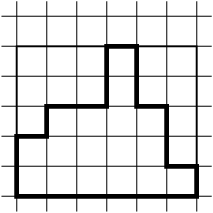
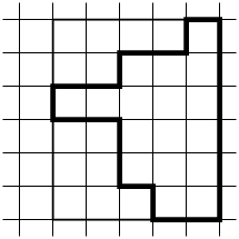
Enumerating self-avoiding polygons according to perimeter or area is an unsolved problem. However, progress has been made in enumerating certain subclasses of self-avoiding polygons. Rectangles coincide with the rectangles of ordinary geometry whose vertices are lattice points and whose edges lie along lattice directions. A rectangle which contains a given polygon, i.e., all steps of the polygon lie inside or on the rectangle, is a bounding rectangle for that polygon. The smallest such rectangle is the minimal bounding rectangle. A polygon whose perimeter equals that of its minimal bounding rectangle is convex. If a convex polygon contains at least one of the corners of its minimal bounding rectangle (for concreteness say the south-west corner) then it is a directed convex polygon. If it contains also the north-east corner, it is a staircase polygon, so called because it is bounded above and below by two staircase-like or directed paths. On the other hand, if it contains two adjacent corners, say the southwest and southeast (northeast and southeast) then it is a stack polygon with horizontal (vertical) orientation. If it contains three corners, then it is a Ferrers graph. Representative examples of different classes of convex polygons are shown in Figure 1.

One way to obtain non-convex polygons is to relax the convexity condition along one direction only. A self-avoiding polygon is column-convex if the intersection of any vertical line with the polygon has at most two connected components. Row-convex polygons are similarly defined. The set of convex polygons is the intersection of the sets of row- and column-convex polygons. Subclasses of column-convex polygons include the bar-graphs which contain the bottom edge of the minimal bounding rectangle, and directed column-convex polygons whose bottom edge is a directed path. Some examples are shown in Figure 2.

A second class of non-convex polygons is made up of four directed paths. A three-choice walk is a self-avoiding walk whose steps are taken in accordance with the three-choice rule which allows a step either to the left or the right or straight ahead after any vertical step, but forbids a right turn after any horizontal step. A polygon formed from such a walk is a three-choice polygon. When the walk returns to its starting point, we don’t specify whether the next step, i.e., the first step, is a valid continuation of the walk. If it is, the result is a staircase polygon; if not, it is an imperfect staircase polygon (see Figure 3(a)). When we refer to three-choice polygons below, we include only the imperfect ones.

A polyomino is a union of connected (sharing an edge) cells of the lattice. We shall consider one class of nonpolygon polyominoes — the staircase polygons with a staircase hole. The outer boundary and the hole are both staircase polygons and must not touch at any point. An example is shown in Figure 3(b).

3.2 Self-reciprocity in polyomino enumeration

For each of the above classes of column-convex polygons, the anisotropic perimeter and area generating function,

G(x,y,q)=\sum_{m\geq 1}\sum_{n\geq 1}\sum_{a\geq 1}C(m,n,a)x^{m}y^{n}q^{a}

(21)

has been computed exactly (see ref. [7] and references therein). Here $C(m,n,a)$ is the number of polygons of the class with $2m$ horizontal bonds, $2n$ vertical bonds and area $a$ . For the classes of convex polygons, the anisotropic perimeter generating function, $G(x,y,1)$ is an algebraic function of the fugacities, $x$ and $y$ , whereas the area generating function, $G(1,1,q)$ is a $q$ -series. For classes of polygons that are only column-convex, both $G(x,y,1)$ and $G(1,1,q)$ [24] are algebraic, but $G(x,y,q)$ involves $q$ -series. A closed-form expression for the three-choice polygon anisotropic perimeter-area generating function is not yet known, but by means of a transfer matrix technique it can be evaluated in polynomial time [9]. The isotropic perimeter generating function, $G(x,x,1)$ is known to have a logarithmic singularity [9], and is therefore not algebraic, but is known to be D-finite. The generating function for staircase polygons with a staircase hole is also not known in closed form. Its properties are expected to be similar in many respects to the generating function for three-choice polygons [11].

We shall be concerned with self-reciprocity properties of the generating functions $H_{m}(y,q)$ that count polygons of width $m$ . We first give two examples.

The area generating function for staircase polygons of width 4 is the following rational function [6]:

H_{4}(q)=\frac{q^{4}(1+2q+4q^{2}+6q^{3}+7q^{4}+6q^{5}+4q^{6}+2q^{7}+q^{8})}{(1-q)^{2}(1-q^{2})^{2}(1-q^{3})^{2}(1-q^{4})}.

It satisfies

H_{4}(1/q)=-H_{4}(q),

and is thus self-reciprocal. Observe that the numerator is not only symmetric (due to self-reciprocity), but also unimodal.

The (half-)vertical perimeter and area generating function for column-convex polygons of width 3 is the following rational function, which can be derived from the general formula of ref. [7]:

	$\displaystyle H_{3}(y,q)=$	$\displaystyle\frac{yq^{3}}{(1-yq)^{4}(1-yq^{2})^{2}(1-yq^{3})}\cdot(y^{6}q^{8}+4y^{5}q^{7}+2y^{5}q^{6}+y^{4}q^{6}-y^{4}q^{4}$
		$\displaystyle-4y^{3}q^{5}-6y^{3}q^{4}-4y^{3}q^{3}-y^{2}q^{4}+y^{2}q^{2}+2yq^{2}+4yq+1).$

It satisfies

H_{3}(1/y,1/q)=-\frac{1}{yq^{3}}H_{3}(y,q)

and hence is self-reciprocal. Again, observe the symmetry of the coefficients in the numerator.

We shall generalize these results to polygons of any width. Table 1 summarizes the self-reciprocity properties we have established. Most of them can be proved in various ways. One can for instance use a closed form expression of the generating function (Section 3.3), or a functional equation that defines it (Section 4); one can also encode the polygons by a sequence of numbers constrained by linear diophantine equations and apply Stanley’s general results (Section 5). We shall see that the last two methods allow us to introduce many additional parameters and obtain self-reciprocity results that significantly generalize those of Table 1.

Class	Self Reciprocity	Inversion Relation
Ferrers	$H_{m}(1/y,1/q)=(-1)^{m}y^{m-2}q^{\frac{m^{2}-3m}{2}}H_{m}(y,q)$	$G(x,y)-y^{2}G(-x/y,1/y)=0$
stack	$H_{m}(1/y,1/q)=-y^{2m-3}q^{m^{2}-2m}H_{m}(y,q)$	$G(x,y)+y^{3}G(x/y^{2},1/y)=0$
staircase	$H_{m}(1/y,1/q)=-y^{m-1}H_{m}(y,q),\ m\geq 2$	$G(x,y,q)+yG(x/y,1/y,1/q)=-x$
directed convex	$H_{m}(1/y)=-y^{m-2}H_{m}(y)$	$G(x,y)+y^{2}G(x/y,1/y)=0$
convex	Not simple	$G(x,y)+y^{3}G(x/y,1/y)=xy-x^{3}y\frac{\partial}{\partial x}\frac{1-x+y}{\Delta(x,y)}$
bargraph	$H_{m}(1/y,1/q)=\frac{(-1)^{m}}{yq^{m}}H_{m}(y,q)$	$G(x,y,q)-yG(-xq,1/y,1/q)=0$
dir. col.-conv.	$H_{m}(1/q)=-\frac{1}{q}H_{m}(q)$	$G(x,q)+qG(x,1/q)=0$
column-convex	$H_{m}(1/y,1/q)=-\frac{1}{yq^{m}}H_{m}(y,q)$	$G(x,y,q)+yG(xq,1/y,1/q)=0$
three-choice	Not simple	$G(x,y,q)+y^{2}G(x/y,1/y,1/q)=\mbox{known}$
SC with SC hole	Not simple	$G(x,y,q)+y^{2}G(x/y,1/y,1/q)=\mbox{known}$

Table 1: Summary of polyomino inversion relations

3.3 Self-reciprocity via generating functions

When a closed form expression for the generating function of some class of polygons is known, it seems natural to use it to demonstrate an inversion relation. Let us take the example of the anisotropic perimeter generating function for directed convex polygons, which is known to be [14]:

G(x,y)=\frac{xy}{{\sqrt{\Delta(x,y)}}}

(22)

with $\Delta(x,y)=1-2x-2y-2xy+x^{2}+y^{2}=(1-y)^{2}\left[1-x(2+2y-x)/(1-y)^{2}\right]$ . Expanding this expression in $x$ gives

	$\displaystyle G(x,y)$	$\displaystyle=$	$\displaystyle\sum_{m\geq 1}H_{m}(y)x^{m}$
		$\displaystyle=$	$\displaystyle\frac{y}{1-y}x+\frac{y(1+y)}{(1-y)^{3}}x^{2}+\frac{y(1+4y+y^{2})}{(1-y)^{5}}x^{3}+\frac{y(1+9y+9y^{2}+y^{3})}{(1-y)^{7}}x^{4}+O(x^{5})$

which suggests that the partial generating functions, $H_{m}(y)$ are self-reciprocal, and more precisely, that $H_{m}(1/y)=-y^{m-2}H_{m}(y)$ . This is equivalent to the inversion relation

G(x,y)+y^{2}G(x/y,1/y)=0,

(23)

which is easily checked from the closed form of the generating function. Note that an explicit expression for $H_{m}(y)$ is given in [6]. The inversion relations for convex polygons and directed column-convex polygons may also be obtained from the expression of their generating function.

The partial generating functions for directed convex polygons, counted by the area, are not self-reciprocal: for instance, the generating function for width $3$ is

q^{3}(1+3q+3q^{2}+2q^{3}+q^{4})/(1-q)^{2}(1-q^{2})^{2}(1-q^{3}).

However, many other classes of column-convex polygons have an inversion relation for the full anisotropic perimeter and area generating function. Since these generating functions are also known in closed form they could be derived as above. However more can be shown, namely that there is a self-reciprocity for any parameter which is a linear function of the vertical heights in the graph. This very general result will be derived in Section 4. Likewise, the inversion relations for three-choice polygons and staircase polygons with a staircase hole, given in Table 1, are also special cases of more general formulae which will be derived in Section 5.

3.4 Using inversion relations to compute
generating functions

As in statistical mechanics, the inversion relation and symmetry, and some general assumptions on analyticity of the generating function, are sometimes sufficient to determine the solution completely. In order to have an algorithm for computing a generating function term by term, it is necessary, but not sufficient, to have some property relating terms of different orders. For our purposes this property will always be $x$ - $y$ symmetry. Thus we restrict our attention to classes of graphs with $x$ - $y$ symmetry, i.e., Ferrers, staircase, directed convex, convex and three-choice polygons, and staircase polygons with a staircase hole. Moreover, we shall only consider the anisotropic perimeter generating function (without area). For the former four classes we will show that the inversion relation provides sufficient additional information to compute the generating function, whereas for the latter two it does not.

The general form of the generating function is

G(x,y)=H_{1}(y)x+H_{2}(y)x^{2}+H_{3}(y)x^{3}+\cdots

(24)

where the partial generating functions, $H_{m}(y)$ are rational functions

H_{m}(y)=\frac{P_{m}(y)}{D_{m}(y)},

(25)

with $D_{m}(0)=1$ . The general form of the inversion relation is

G(x,y)\pm y^{\alpha}G(\epsilon x/y,1/y)=\text{RHS}

(26)

where $\alpha$ is an integer and RHS is zero or some simple function. It is equivalent to a self-reciprocity relation of the form

H_{m}(1/y)\pm\epsilon^{m}y^{m-\alpha}H_{m}(y)=\text{RHS}.

Whether the inversion relation is sufficient to compute the generating function depends on the value of the exponent $\alpha$ and on the degree of the denominator, $D_{m}(y)$ . Direct proof of the denominator form can often be obtained. For Ferrers graphs, it is easily shown that $D_{m}(y)=(1-y)^{m}$ . For staircase polygons, one finds $D_{m}(y)=(1-y)^{2m-1}$ . The same denominator form holds for directed convex and convex polygons also. For the three-choice polygons and staircase polygons with a staircase hole it can be shown that the denominators are

D_{m}(y)=\begin{cases}(1-y)^{2m-1}(1+y)^{2m-7}&\text{$m$ even}\\ (1-y)^{2m-1}(1+y)^{2m-8}&\text{$m$ odd.}\end{cases}

(27)

We assume that in general we know the denominator form either empirically or by rigorous proof, and that $D_{m}(y)$ is of degree $d_{m}$ .

Now we proceed inductively, following Baxter [2]. If we have already computed the coefficient functions $H_{1}(y),\ldots,H_{m-1}(y)$ in the expansion (24) and if $x$ - $y$ symmetry holds, we also know the coefficients of $y,y^{2},\ldots,y^{m-1}$ in the expansion of $G(x,y)$ . In particular, we can compute the coefficients of $y,y^{2},\ldots,y^{m-1}$ in the numerator polynomial $P_{m}(y)$ . In order to obtain the unknown coefficients of $P_{m}(y)$ , we must be able to express them in terms of the known ones by means of the inversion relation. Writing $P_{m}(y)=\sum_{k}a_{k}y^{k}$ , and using $D_{m}(1/y)=\pm y^{-d_{m}}D_{m}(y)$ , the inversion relation fixes the value of the combinations of coefficients, $a_{k}\pm a_{\ell}$ , with $k+\ell=\alpha+d_{m}-m$ . Hence the determination of all the coefficients $a_{k}$ is possible if and only if the arithmetic condition holds:

d_{m}<3m-\alpha.

(28)

This condition is seen to hold for all the classes of convex polygons we have looked at, since $d_{m}\leq 2m-1$ , but not for three-choice polygons or staircase polygons with a staircase hole, since $d_{m}\sim 4m$ .

4 Self-reciprocity via Temperley methodology

We consider column-convex polygons as pairs of partially directed paths having the same endpoints, as indicated in Figure 4.

Let $P$ be a column-convex polygon of width $m$ . For $0\leq i\leq m$ , we denote by ${\overline{N}}_{i}$ (resp. ${\overline{S}}_{i}$ ) the number of north (resp. south) steps in the top path $\overline{\gamma}$ at abscissa $i$ . For $0\leq i\leq m$ , we denote by ${\underline{N}}_{i}$ (resp. ${\underline{S}}_{i}$ ) the number of north (resp. south) steps of the bottom path $\underline{\gamma}$ at abscissa $i$ . We choose the end points of the paths in such a way that ${\underline{N}}_{0}={\underline{S}}_{0}={\overline{N}}_{m}={\overline{S}}_{m}={\overline{S}}_{0}={\underline{S}}_{m}=0$ . Note that

\sum_{k=0}^{m}({\overline{N}}_{k}+{\underline{S}}_{k}-{\overline{S}}_{k}-{\underline{N}}_{k})=0.

We notice that all standard statistics are linear functions of the ${\overline{N}}_{i},{\overline{S}}_{i},{\underline{N}}_{i}$ and ${\underline{S}}_{i}$ . For instance, the vertical perimeter of the polygon is

	$\displaystyle 2n$	$\displaystyle=\sum_{k=0}^{m}({\overline{N}}_{k}+{\underline{S}}_{k}+{\overline{S}}_{k}+{\underline{N}}_{k})$
		$\displaystyle=2\,\sum_{k=0}^{m}({\overline{N}}_{k}+{\underline{S}}_{k}).$		(29)

The height of the $i^{\text{th}}$ column of the polygon is, for $1\leq i\leq m$ ,

\displaystyle h_{i}

\displaystyle=\sum_{k=0}^{i-1}({\overline{N}}_{k}+{\underline{S}}_{k}-{\overline{S}}_{k}-{\underline{N}}_{k}),

and the area of the polygon is

a=\sum_{k=0}^{m}(m-k)({\overline{N}}_{k}+{\underline{S}}_{k}-{\overline{S}}_{k}-{\underline{N}}_{k}).

(30)

Theorem 4.1.

Let $\cal P$ be one of the following sets: Ferrers diagrams, stacks (drawn as in Figure 1(c)), staircase polygons, bar-graphs, column-convex polygons. Let ${\cal P}_{m}$ be the subset of $\cal P$ containing all polygons of width $m$ . Let $F_{m}$ be the generating function for polygons in the set ${\cal P}_{m}$ :

F_{m}(\boldsymbol{{\overline{y}}},\boldsymbol{{\overline{z}}},\boldsymbol{{\underline{y}}},\boldsymbol{{\underline{z}}})=\sum_{P\in{\cal P}_{m}}\boldsymbol{{\overline{y}}}^{\mathbf{{\overline{N}}}}\boldsymbol{{\overline{z}}}^{\mathbf{{\overline{S}}}}\boldsymbol{{\underline{y}}}^{\mathbf{{\underline{N}}}}\boldsymbol{{\underline{z}}}^{\mathbf{{\underline{S}}}}.

Then $F_{m}$ is a rational function, and it is self-reciprocal:

F_{m}(1/\boldsymbol{{\overline{y}}},1/\boldsymbol{{\overline{z}}},1/\boldsymbol{{\underline{y}}},1/\boldsymbol{{\underline{z}}})=C_{m}F_{m}(\boldsymbol{{\overline{y}}},\boldsymbol{{\overline{z}}},\boldsymbol{{\underline{y}}},\boldsymbol{{\underline{z}}}),

(31)

with

C_{m}=\left\{\begin{array}[]{ll}\displaystyle\frac{(-1)^{m}{\underline{y}}_{m}^{m-2}}{{\overline{y}}_{0}}\prod_{i=1}^{m-1}{\overline{y}}_{i}&\hbox{for Ferrers graphs,}\\ &\\ \displaystyle-\frac{{\underline{y}}_{m}^{2m-3}}{{\overline{y}}_{0}}\prod_{i=1}^{m-1}{\overline{y}}_{i}{\underline{z}}_{i}&\hbox{for stacks,}\\ &\\ \displaystyle-\prod_{i=1}^{m-1}{\underline{y}}_{i}{\overline{y}}_{i}&\hbox{for staircase polygons }(m\geq 2),\\ &\\ \displaystyle\frac{(-1)^{n}}{{\overline{y}}_{0}{\underline{y}}_{m}}&\hbox{for bar-graphs},\\ &\\ \displaystyle-\frac{1}{{\overline{y}}_{0}{\underline{y}}_{m}}&\hbox{for column-convex polygons}.\\ \end{array}\right.

The proof of the theorem is based on the so-called Temperley approach for counting column-convex polygons [24], combined with the systematic use of formal power series [7]. Here we provide only the proof for column-convex polygons, since the others are very similar.

We commence by showing that the partial generating functions for column-convex polygons, $V_{m}(\boldsymbol{{\overline{y}}},\boldsymbol{{\overline{z}}},\boldsymbol{{\underline{y}}},\boldsymbol{{\underline{z}}})$ , can be computed inductively.

Proposition 4.2.

Let $V_{m}(\boldsymbol{{\overline{y}}},\boldsymbol{{\overline{z}}},\boldsymbol{{\underline{y}}},\boldsymbol{{\underline{z}}})$ be the generating function for column-convex polygons of width $m$ . Let us denote it, for the sake of simplicity, $V_{m}({\underline{y}}_{m})$ . Then the series $V_{m}({\underline{y}}_{m})$ can be defined inductively by:

V_{1}({\underline{y}}_{1})=\frac{{\overline{y}}_{0}{\underline{y}}_{1}}{1-{\overline{y}}_{0}{\underline{y}}_{1}}

and

		$\displaystyle V_{m+1}({\underline{y}}_{m+1})=\frac{(1-{\underline{y}}_{m}{\underline{z}}_{m})(1-{\overline{y}}_{m}{\overline{z}}_{m})V_{m}({\underline{y}}_{m+1})}{(1-{\underline{y}}_{m+1}{\overline{y}}_{m})(1-{\underline{y}}_{m+1}{\underline{z}}_{m})(1-{\underline{y}}_{m+1}^{-1}{\underline{y}}_{m})(1-{\underline{y}}_{m+1}^{-1}{\overline{z}}_{m})}$
		$\displaystyle\quad+\frac{({\overline{z}}_{m}-{\underline{y}}_{m+1}{\underline{y}}_{m}{\underline{z}}_{m})V_{m}({\overline{z}}_{m})}{(1-{\underline{y}}_{m+1}{\underline{z}}_{m})(1-{\underline{y}}_{m+1}^{-1}{\overline{z}}_{m})({\underline{y}}_{m}-{\overline{z}}_{m})}+\frac{({\underline{y}}_{m}-{\underline{y}}_{m+1}{\overline{y}}_{m}{\overline{z}}_{m})V_{m}({\underline{y}}_{m})}{(1-{\underline{y}}_{m+1}{\overline{y}}_{m})(1-{\underline{y}}_{m+1}^{-1}{\underline{y}}_{m})({\overline{z}}_{m}-{\underline{y}}_{m})}.$

Proof. The basic idea is build a polygon of width $m+1$ by adding a new column to a polygon of width $m$ [7]. It is convenient to use Hadamard products to establish the functional equation.

Let $F(t)=\sum f_{h}t^{h}$ and $R(t)=\sum r_{h}t^{h}$ be two formal power series in $t$ with coefficients in a ring $A$ . We denote by $F(t)\odot R(t)$ the Hadamard product of $F(t)$ and $R(t)$ , evaluated at $t=1$ :

F(t)\odot R(t)=\sum f_{h}r_{h}.

In what follows, $f_{h}$ (resp. $r_{h}$ ) will be the generating function for some column-convex polygons whose rightmost (resp. leftmost) column has height $h$ , so that $F(t)\odot R(t)$ will count polygons obtained by matching the rightmost column of a polygon of type $F$ with the leftmost column of a polygon of type $R$ . Also, $R(t)$ will be a rational function of $t$ . We shall use the following simple identity:

F(t)\odot\frac{1}{1-at}=F(a).

The expression for $V_{1}({\underline{y}}_{1})$ is obvious. We build a column-convex polygon of width $m+1$ as follows: we take a polygon of width $m$ and match its rightmost column with the leftmost column of a column-convex polygon of width $2$ .

This is illustrated by Figure 5, which shows that

V_{m+1}({\underline{y}}_{m+1})=V_{m}(t)\odot R(t),

(32)

where

	$\displaystyle R(t)=$	$\displaystyle\frac{t{\underline{y}}_{m+1}}{1-t{\underline{y}}_{m+1}}\cdot\frac{1}{1-{\underline{y}}_{m+1}{\overline{y}}_{m}}\cdot\frac{1}{1-{\underline{y}}_{m+1}{\underline{z}}_{m}}+\frac{t{\underline{y}}_{m+1}}{1-t{\underline{y}}_{m+1}}\cdot\frac{1}{1-{\underline{y}}_{m+1}{\overline{y}}_{m}}\cdot\frac{t{\underline{y}}_{m}}{1-t{\underline{y}}_{m}}$
		$\displaystyle+\frac{t{\underline{y}}_{m+1}}{1-t{\underline{y}}_{m+1}}\cdot\frac{t{\overline{z}}_{m}}{1-t{\overline{z}}_{m}}\cdot\frac{1}{1-{\underline{y}}_{m+1}{\underline{z}}_{m}}+\frac{t{\underline{y}}_{m+1}}{1-t{\underline{y}}_{m+1}}\cdot\frac{t{\overline{z}}_{m}}{1-t{\overline{z}}_{m}}\cdot\frac{t{\underline{y}}_{m}}{1-t{\underline{y}}_{m}}$

is the generating function for column-convex polygons of width $2$ . In order to determine the coefficient $r_{h}$ of $t^{h}$ in $R(t)$ , we expand $R(t)$ in partial fractions of $t$ :

	$\displaystyle R(t)=$	$\displaystyle\frac{{\underline{z}}_{m}{\overline{y}}_{m}{\underline{y}}_{m+1}^{2}}{(1-{\underline{y}}_{m+1}{\overline{y}}_{m})(1-{\underline{y}}_{m+1}{\underline{z}}_{m})}$
		$\displaystyle+\frac{(1-{\underline{y}}_{m}{\underline{z}}_{m})(1-{\overline{y}}_{m}{\overline{z}}_{m})}{(1-{\underline{y}}_{m+1}{\overline{y}}_{m})(1-{\underline{y}}_{m+1}{\underline{z}}_{m})(1-{\underline{y}}_{m+1}^{-1}{\underline{y}}_{m})(1-{\underline{y}}_{m+1}^{-1}{\overline{z}}_{m})}\cdot\frac{1}{1-t{\underline{y}}_{m+1}}$
		$\displaystyle+\frac{({\overline{z}}_{m}-{\underline{y}}_{m+1}{\underline{y}}_{m}{\underline{z}}_{m})}{(1-{\underline{y}}_{m+1}{\underline{z}}_{m})(1-{\underline{y}}_{m+1}^{-1}{\overline{z}}_{m})({\underline{y}}_{m}-{\overline{z}}_{m})}\cdot\frac{1}{1-t{\overline{z}}_{m}}$
		$\displaystyle+\frac{({\underline{y}}_{m}-{\underline{y}}_{m+1}{\overline{y}}_{m}{\overline{z}}_{m})}{(1-{\underline{y}}_{m+1}{\overline{y}}_{m})(1-{\underline{y}}_{m+1}^{-1}{\underline{y}}_{m})({\overline{z}}_{m}-{\underline{y}}_{m})}\cdot\frac{1}{1-t{\underline{y}}_{m}}.$

Note that $V_{m}(0)=0$ . We now combine eqn. ?? with the above expression for $R(t)$ to obtain the announced expression for $V_{m+1}({\underline{y}}_{m+1})$ .

Proof of Theorem 4.1. Induction on $m$ using the functional equation of Proposition 4.2 shows that the partial generating functions for column-convex polygons satisfy:

{V_{m}}(1/\boldsymbol{{\overline{y}}},1/\boldsymbol{{\overline{z}}},1/\boldsymbol{{\underline{y}}},1/\boldsymbol{{\underline{z}}})=-\frac{1}{{\overline{y}}_{0}{\underline{y}}_{m}}V_{m}(\boldsymbol{{\overline{y}}},\boldsymbol{{\overline{z}}},\boldsymbol{{\underline{y}}},\boldsymbol{{\underline{z}}}).

We proceed similarly for the other families: the functional equation is obtained by setting some of the variables ${\overline{y}}_{i},{\underline{y}}_{i},{\overline{z}}_{i}$ and ${\underline{z}}_{i}$ to $0$ . Then, an inductive argument yields the self-reciprocity result.

It would be tempting to write that the self-reciprocity of $V_{m}$ implies the self-reciprocity of, say, the generating function for staircase polygons, obtained by setting ${\underline{z}}_{i}$ and ${\overline{z}}_{i}$ to $0$ in $V_{m}$ . But replacing a variable by $0$ in a self-reciprocal rational function might break the self-reciprocity: for instance, take $P(y_{1},y_{2})=1+y_{1}+2y_{1}^{2}+2y_{2}+y_{1}y_{2}+y_{1}^{2}y_{2}.$ Then

P(1/y_{1},1/y_{2})=\frac{1}{y_{1}^{2}y_{2}}P(y_{1},y_{2}),

but $P(y_{1},0)=1+y_{1}+2y_{1}^{2}$ is not self-reciprocal.

However, the following simple lemma gives a useful stability property of self-reciprocal rational functions.

Lemma 4.3.

Let $F(y_{1},\ldots,y_{n})$ be a self-reciprocal rational function. Let ${\mathbf{\mathsf{A}}}$ be an $m\times n$ integer matrix. Let ${\boldsymbol{u}}=(u_{1},\ldots,u_{m})$ , and define ${\boldsymbol{u}}^{\mathbf{\mathsf{A}}}$ to be the $n$ -tuple whose $i^{\text{th}}$ coordinate is $\prod_{k}u_{k}^{a_{ki}}$ . Then the series $G({\boldsymbol{u}})=F({\boldsymbol{u}}^{\mathbf{\mathsf{A}}})$ , if defined, is self-reciprocal in the variables $u_{i}$ . More precisely, if $F(1/{\boldsymbol{y}})=\pm{\boldsymbol{y}}^{\boldsymbol{\beta}}F({\boldsymbol{y}})$ then $G(1/{\boldsymbol{u}})=\pm{\boldsymbol{u}}^{{\mathbf{\mathsf{A}}}{\boldsymbol{\beta}}}G({\boldsymbol{u}})$ .

From Theorem 4.1 and Lemma 4.3 we immediately deduce:

Corollary 4.4.

For any of the sets $\cal P$ listed in Theorem 4.1, and any statistics on column-convex polygons that can be expressed as linear functions of the quantities $\mathbf{{\overline{N}}},\mathbf{{\overline{S}}},\mathbf{{\underline{N}}},\mathbf{{\underline{S}}}$ , the generating function for polygons in the set ${\cal P}_{m}$ according to these statistics is a self-reciprocal rational function.

This corollary allows us to complete the top part of Table 1. Let us, for instance, derive the inversion relation satisfied by the tri-variate generating function $G(x,y,q)$ for column-convex polygons, taking into account the usual parameters of interest: horizontal and vertical half-perimeters (variables $x$ and $y$ ), and area (variable $q$ ).

Eqns. ?? and ?? express the vertical perimeter and the area in terms of the quantities $\mathbf{{\overline{N}}},\mathbf{{\underline{N}}},\mathbf{{\overline{S}}}$ and $\mathbf{{\underline{S}}}$ . They imply that the (half) vertical perimeter and area generating function $H_{m}(y,q)$ for column-convex polygons of width $m$ is

H_{m}(y,q)=V_{m}(\mathbf{{\overline{N}}},\mathbf{{\overline{S}}},\mathbf{{\underline{N}}},\mathbf{{\underline{S}}})

where ${\overline{y}}_{k}={\underline{z}}_{k}=yq^{m-k}$ and ${\underline{y}}_{k}={\overline{z}}_{k}=q^{-(m-k)}$ . Theorem 4.1 then gives

H_{m}(1/y,1/q)=-\frac{1}{yq^{m}}H_{m}(y,q),

which implies

G(x,y,q)+yG(xq,1/y,1/q)=0.

(33)

Note that in the first two self-reciprocity relations of Table 1, the exponent of $q$ depends quadratically on the width. For this reason, they only yield an inversion relation for $q=1$ .

5 Self-reciprocity via Stanley’s general results

5.1 Linear homogeneous diophantine systems

Stanley has analyzed the situation where the objects to be counted correspond to integer solutions of a system of linear equations with integer coefficients (linear diophantine system) subject to a set of constraints. He has established certain conditions under which reciprocity relations will hold between two combinatorics problems defined by the same linear diophantine system but by different sets of constraints, and also conditions under which the solution to a given problem will be self-reciprocal [20, 22].

Consider the linear homogeneous diophantine system (LHD-system),

{\boldsymbol{\Phi}}{\boldsymbol{\alpha}}={\mathbf{0}}

(34)

in the unknowns ${\boldsymbol{\alpha}}=(\alpha_{1},\ldots,\alpha_{s})$ with ${\boldsymbol{\Phi}}$ a matrix of integers having $p$ rows and $s$ columns and ${\mathbf{0}}$ a $p$ -tuple of zeros. The corank $\kappa$ of the system is defined to be $s-\mathrm{rank}({\boldsymbol{\Phi}})$ . For a linearly independent system, $\kappa=s-p$ . Let $S$ be a set of integer solutions to eqn. (34). We define the generating function, $S({\boldsymbol{y}})$ , as the formal power series

S({\boldsymbol{y}})=\sum_{{\boldsymbol{\alpha}}\in S}{\boldsymbol{y}}^{\boldsymbol{\alpha}}

(35)

where ${\boldsymbol{y}}=(y_{1},\ldots,y_{s})$ is a vector of fugacities associated with the unknowns in eqn. (34).

In our applications, we find two types of constraints on the unknowns, $\alpha_{j}$ . Certain of the unknowns, $\alpha_{j}$ , are required to be strictly positive while the rest are required to be non-negative. Conveniently, precisely these kinds of constraints have been treated by Stanley. Let the unknowns be ${\boldsymbol{\alpha}}=({\boldsymbol{\gamma}},{\boldsymbol{\delta}})\equiv{\boldsymbol{\gamma}}\oplus{\boldsymbol{\delta}}$ where ${\boldsymbol{\gamma}}$ is an $n$ -tuple and ${\boldsymbol{\delta}}$ is an $(s-n)$ -tuple. Likewise let ${\boldsymbol{y}}=({\boldsymbol{u}},{\boldsymbol{v}})$ . In what follows, the notation, ${\boldsymbol{\delta}}>{\mathbf{0}}$ , means that all coordinates of ${\boldsymbol{\delta}}$ are positive.

Proposition 5.1.

Let $E$ be the set of integer solutions, $({\boldsymbol{\gamma}},{\boldsymbol{\delta}})$ , to a linear homogeneous diophantine system of corank $\kappa$ , such that ${\boldsymbol{\gamma}}\geq{\mathbf{0}}$ and ${\boldsymbol{\delta}}>{\mathbf{0}}$ . Let $\overline{E}$ be the set of solutions to the same system with ${\boldsymbol{\gamma}}>{\mathbf{0}}$ and ${\boldsymbol{\delta}}\geq{\mathbf{0}}$ . If the system has an integer solution, $({\boldsymbol{\gamma}},{\boldsymbol{\delta}})$ such that ${\boldsymbol{\gamma}}>0$ and ${\boldsymbol{\delta}}<0$ , then $E({\boldsymbol{u}},{\boldsymbol{v}})$ and $\overline{E}({\boldsymbol{u}},{\boldsymbol{v}})$ are rational functions obeying the reciprocity relation

\overline{E}({\boldsymbol{u}},{\boldsymbol{v}})=(-1)^{\kappa}E(1/{\boldsymbol{u}},1/{\boldsymbol{v}}).

(36)

Proof. This is Proposition 8.3 of ref. [20] and the proof is given there.

Proposition 36 can be specialized to obtain a self-reciprocity condition, which will be our main tool in the derivations to follow.

Corollary 5.2.

A sufficient condition for the function $E({\boldsymbol{u}},{\boldsymbol{v}})$ to be self-reciprocal is that the linear homogeneous diophantine system has the solution $({\boldsymbol{\gamma}},{\boldsymbol{\delta}})=({\mathbf{1}},-{\mathbf{1}})$ . In this case

E(1/{\boldsymbol{u}},1/{\boldsymbol{v}})=(-1)^{\kappa}\frac{{\boldsymbol{u}}^{\mathbf{1}}}{{\boldsymbol{v}}^{\mathbf{1}}}E({\boldsymbol{u}},{\boldsymbol{v}}).

(37)

Proof. Since the solution $({\mathbf{1}},-{\mathbf{1}})$ satisfies the conditions of Proposition 36, the reciprocity result (36) holds. The result follows immediately from the shift $({\boldsymbol{\gamma}},{\boldsymbol{\delta}})\rightarrow({\boldsymbol{\gamma}}+{\mathbf{1}},{\boldsymbol{\delta}}-{\mathbf{1}})$ which establishes a bijection between the sets $E$ and $\overline{E}$ .

Since the conditions of the corollary are sufficient but not necessary, it is often possible to find a perfectly valid LHD-system describing a given self-reciprocal generating function, $E({\boldsymbol{u}},{\boldsymbol{v}})$ , which does not admit the solution $({\mathbf{1}},-{\mathbf{1}})$ . Hence we are faced with the problem of finding a suitable LHD-system which satisfies the corollary. A useful heuristic is to start with an LHD-system in many unknowns, and selectively eliminate those unknowns whose constraints are not independent of the constraints on the other unknowns. In all the cases we will consider, the resulting system will satisfy the conditions of Corollary 37. We do not justify this heuristic here. In a paper subsequent to ref. [20], Stanley [21] develops a more comprehensive theory which overcomes these difficulties, and which additionally gives “correction” terms for systems in which self-reciprocity fails to hold. We have not yet explored the ramifications of this theory.

Before applying the above result to staircase polygons with a staircase hole or to three-choice polygons, we use it to derive the reciprocity relation for ordinary staircase polygons of width three. This will serve to illustrate all the basic ingredients of the method.

Example 5.3.

Staircase polygons of width three can be characterized by the heights ${\overline{N}}_{1}$ , ${\overline{N}}_{2}$ , ${\underline{N}}_{1}$ , ${\underline{N}}_{2}$ , $M_{0}$ , $M_{1}$ , $M_{2}$ and $M_{3}$ , as shown in Figure 6. Decomposing the polygon into three columns, and imposing the condition that each column be as high on the left as it is on the right, we obtain the linear homogeneous diophantine system


$\displaystyle M_{0}-M_{1}-{\underline{N}}_{1}$	$\displaystyle=0$	(38a)
$\displaystyle M_{1}+{\overline{N}}_{1}-M_{2}-{\underline{N}}_{2}$	$\displaystyle=0$	(38b)
$\displaystyle M_{2}+{\overline{N}}_{2}-M_{3}$	$\displaystyle=0.$	(38c)

All heights must be nonnegative, but the self-avoidance condition additionally requires that the $M_{j}$ be positive. The constraints $M_{0}>0$ and $M_{3}>0$ are actually redundant, since they follow from eqns. (38a,38c) and the constraints on the remaining unknowns, namely

	$\displaystyle{\overline{N}}_{1},{\overline{N}}_{2},{\underline{N}}_{1},{\underline{N}}_{2}$	$\displaystyle\geq 0$
	$\displaystyle M_{1},M_{2}$	$\displaystyle>0.$		(39)

Since the constraints on $M_{0}$ and $M_{3}$ play no role in the solution, we are free to eliminate these unknowns, and it turns out to be necessary to do so in order to apply Corollary 37. We are left with the single equation (38b) in the six independent unknowns ${\boldsymbol{\gamma}}=({\overline{N}}_{1},{\overline{N}}_{2},{\underline{N}}_{1},{\underline{N}}_{2})$ and ${\boldsymbol{\delta}}=(M_{1},M_{2})$ . Let us associate to the unknown ${\overline{N}}_{i}$ (resp. ${\underline{N}}_{i}$ , $M_{i}$ ) the fugacity ${\overline{y}}_{i}$ (resp. ${\underline{y}}_{i}$ , $z_{i}$ ).

Let $E^{\prime}$ be the set of solutions to eqn. (38b) subject to the the constraints ${\boldsymbol{\gamma}}\geq 0$ and ${\boldsymbol{\delta}}>0$ . Since ${\boldsymbol{\gamma}}={\mathbf{1}}$ , ${\boldsymbol{\delta}}=-{\mathbf{1}}$ is a solution to eqn. (38b), Corollary 37 tells us that $E^{\prime}(\boldsymbol{{\overline{y}}},\boldsymbol{{\underline{y}}},{\boldsymbol{z}})$ is self-reciprocal,

E^{\prime}(1/\boldsymbol{{\overline{y}}},1/\boldsymbol{{\underline{y}}},1/{\boldsymbol{z}})=-\frac{{\overline{y}}_{1}{\overline{y}}_{2}{\underline{y}}_{1}{\underline{y}}_{2}}{z_{1}z_{2}}E^{\prime}(\boldsymbol{{\overline{y}}},\boldsymbol{{\underline{y}}},{\boldsymbol{z}}).

(40)

Equations (38a,38c) imply that to account for the dependent parameters $M_{0}$ and $M_{3}$ , we make the substitutions $z_{1}\rightarrow z_{0}z_{1}$ , ${\underline{y}}_{1}\rightarrow z_{0}{\underline{y}}_{1}$ , $z_{2}\rightarrow z_{2}z_{3}$ and ${\overline{y}}_{2}\rightarrow z_{3}{\overline{y}}_{2}$ . Applying Lemma 4.3, we obtain for the set $E$ of nonnegative solutions to (38a,38b,38c) such that $\mathbf{M}>{{\mathbf{0}}}$ :

E(1/\boldsymbol{{\overline{y}}},1/\boldsymbol{{\underline{y}}},1/{\boldsymbol{z}})=-\frac{{\overline{y}}_{1}{\overline{y}}_{2}{\underline{y}}_{1}{\underline{y}}_{2}}{z_{1}z_{2}}E(\boldsymbol{{\overline{y}}},\boldsymbol{{\underline{y}}},{\boldsymbol{z}}).

(41)

Notice that reintroducing the dependent unknowns has not changed the constant factor. This feature holds as well in the more complicated models we will look at. The result (41) may be verified by inspection of the explicit expression for the generating function

E(\boldsymbol{{\overline{y}}},\boldsymbol{{\underline{y}}},{\boldsymbol{z}})=\frac{z_{0}z_{1}z_{2}z_{3}(1-{\overline{y}}_{1}z_{0}z_{1}z_{2}z_{3}{\underline{y}}_{2})}{(1-z_{0}{\underline{y}}_{1})(1-z_{0}z_{1}{\underline{y}}_{2})(1-{\overline{y}}_{1}{\underline{y}}_{2})(1-z_{0}z_{1}z_{2}z_{3})(1-{\overline{y}}_{1}z_{2}z_{3})(1-{\overline{y}}_{2}z_{3})}.

5.2 Applications

We now apply the methods of Section 5.1 to staircase polygons with a staircase hole and to three-choice polygons. All the essential steps have already been seen in the derivation of the reciprocity result for staircase polygons of width three. They are

1.

Set up a linear homogeneous diophantine system by decomposing the polyomino into width one rectangles and imposing the condition that the left and right sides of each rectangle have equal height.
2.

Sort the unknowns into three classes, ${\boldsymbol{\gamma}}$ , ${\boldsymbol{\delta}}$ and ${\boldsymbol{\tau}}$ , according to whether they are constrained to be nonnegative, constrained to be positive or constrained by conditions on the other unknowns.
3.

Use Gaussian elimination to remove the unknowns in ${\boldsymbol{\tau}}$ .
4.

Verify that the resulting system is solved by setting all members of ${\boldsymbol{\gamma}}$ equal to one and all members of ${\boldsymbol{\delta}}$ equal to minus one. Apply Corollary 37 to obtain the self-reciprocity result for the reduced system.
5.

Reintroduce the unknowns in the set ${\boldsymbol{\tau}}$ by means of Lemma 4.3.

We can define three widths for a staircase polygon with a staircase hole: the distance from the left edge of the figure to the left edge of the hole, $k$ , the distance from the left edge of the figure to the right edge of the hole, $\ell$ , and the width of the entire figure, $m$ . Note that $0<k<\ell<m$ . Recall that for staircase polygons the figures of width one were an exceptional case which did not obey the same reciprocity result as the general case. The staircase polygons with a hole of width one are also an exceptional case, which we must exclude. We thus impose the additional condition $\ell-k>1$ . A figure with given $k$ , $\ell$ and $m$ is specified by the following dimensions, as shown in Figure 7(a),

1.

heights ${\underline{N}}_{j}$ and ${\overline{N}}_{j}$ of the lower and upper perimeter segments of the polygon, $1\leq j\leq m-1$ ,
2.

interior heights $M_{j}$ to the left and right of, and within, the hole, $0\leq j\leq m$ ,
3.

heights ${\underline{H}}_{j}$ and ${\overline{H}}_{j}$ of the lower and upper perimeter segments of the hole, $k+1\leq j\leq\ell-1$ ,
4.

interior heights ${\underline{M}}_{j}$ and ${\overline{M}}_{j}$ below and above the hole, $k\leq j\leq\ell$ .

Three-choice polygons can be regarded as staircase polygons with a hole which doesn’t close. The width $k$ has the same meaning as above, $\ell$ denotes the ultimate horizontal extent of the branch of the figure above the hole, and $m$ denotes the ultimate horizontal extent of the branch below the hole. Note that $\ell\geq k$ and $m>k$ . Again an exceptional case, $m=k+1$ , must be excluded. Hence we impose the restriction $m>k+1$ . The labeling of the vertical dimensions follows, with a few obvious modifications, the pattern of staircase polygons with a staircase hole and is shown in Figure 7(b). In particular, the heights $M_{j}$ within the hole are defined only for $j\leq\min(\ell,m)$ . When $\ell=k$ the unknowns ${\overline{M}}_{j}$ and ${\overline{H}}_{j}$ do not appear. This special case is treated separately.

As in the case of column-convex polygons, the standard statistics are linear in these heights. The (half-)vertical perimeter for staircase polygons with a staircase hole is given by

n=M_{0}+\sum_{j=1}^{m-1}{\overline{N}}_{j}+M_{k}+\sum_{j=k+1}^{\ell-1}{\overline{H}}_{j}

(42)

and the area is given by

a=M_{0}+\sum_{j=1}^{k-1}(M_{j}+{\overline{N}}_{j})+\sum_{j=k+1}^{\ell}({\underline{N}}_{j}+{\underline{M}}_{j})+\sum_{j=k}^{\ell-1}({\overline{M}}_{j}+{\overline{N}}_{j})+\sum_{j=\ell+1}^{m-1}({\underline{N}}_{j}+M_{j})+M_{m}.

(43)

In what follows, we associate to the unknowns ${\overline{N}}_{i}$ (resp. ${\underline{N}}_{i}$ , ${\overline{H}}_{i}$ , ${\underline{H}}_{i}$ , $M_{i}$ , ${\overline{M}}_{i}$ , ${\underline{M}}_{i}$ ) the fugacities ${\overline{y}}_{i}$ (resp. ${\underline{y}}_{i},{\overline{w}}_{i},{\underline{w}}_{i},z_{i},{\overline{z}}_{i},{\underline{z}}_{i}$ ).

Proposition 5.4.

Let $E_{k,\ell,m}(\boldsymbol{{\overline{y}}},\boldsymbol{{\underline{y}}},\boldsymbol{{\overline{w}}},\boldsymbol{{\underline{w}}},{\boldsymbol{z}},\boldsymbol{{\overline{z}}},\boldsymbol{{\underline{z}}})$ be the generating function for staircase polygons with a staircase hole where $k$ , $\ell$ and $m$ are the widths defined above. Then if $\ell-k>1$ , the generating function $E_{k,\ell,m}(\boldsymbol{{\overline{y}}},\boldsymbol{{\underline{y}}},\boldsymbol{{\overline{w}}},\boldsymbol{{\underline{w}}},{\boldsymbol{z}},\boldsymbol{{\overline{z}}},\boldsymbol{{\underline{z}}})$ is self-reciprocal,

E_{k,\ell,m}(1/\boldsymbol{{\overline{y}}},1/\boldsymbol{{\underline{y}}},1/\boldsymbol{{\overline{w}}},1/\boldsymbol{{\underline{w}}},1/{\boldsymbol{z}},1/\boldsymbol{{\overline{z}}},1/\boldsymbol{{\underline{z}}})=\ \ \ \ \ \ \ \ \ \ \ \ \ \ \ \ \ \ \ \ \ \ \ \ \ \ \ \ \ \ \ \ \ \ \ \ \ \ \ \ \ \ \ \ \ \ \ \

\ \ \ \ \ \ \ \ \ \ \ \ -\frac{z_{k}z_{\ell}\prod_{j=1}^{m-1}({\overline{y}}_{j}{\underline{y}}_{j})\prod_{j=k+1}^{\ell-1}({\overline{w}}_{j}{\underline{w}}_{j})}{\prod_{j=1}^{m-1}z_{j}\prod_{j=k+1}^{\ell}{\underline{z}}_{j}\prod_{j=k}^{\ell-1}{\overline{z}}_{j}}E_{k,\ell,m}(\boldsymbol{{\overline{y}}},\boldsymbol{{\underline{y}}},\boldsymbol{{\overline{w}}},\boldsymbol{{\underline{w}}},{\boldsymbol{z}},\boldsymbol{{\overline{z}}},\boldsymbol{{\underline{z}}}).

(44)

Proof. The linear homogeneous diophantine system is the union of five sets of equations which we label $L_{1}$ – $L_{5}$ . The regions to the left and right of the hole give $L_{1}$ and $L_{2}$ , the regions below and above the hole give $L_{3}$ and $L_{4}$ and the inside of the hole gives $L_{5}$ :

$\displaystyle L_{1}$	$\displaystyle=\begin{cases}M_{0}-M_{1}-{\underline{N}}_{1}=0\\ M_{j}+{\overline{N}}_{j}-M_{j+1}-{\underline{N}}_{j+1}=0\qquad\text{for $1\leq j\leq k-2$}\\ M_{k-1}+{\overline{N}}_{k-1}-{\overline{M}}_{k}-M_{k}-{\underline{M}}_{k}-{\underline{N}}_{k}=0\end{cases}$
$\displaystyle L_{2}$	$\displaystyle=\begin{cases}{\underline{M}}_{\ell}+M_{\ell}+{\overline{M}}_{\ell}+{\overline{N}}_{\ell}-M_{\ell+1}-{\underline{N}}_{\ell+1}=0\\ M_{j}+{\overline{N}}_{j}-M_{j+1}-{\underline{N}}_{j+1}=0\qquad\text{for $\ell+1\leq j\leq m-2$}\\ M_{m-1}+{\overline{N}}_{m-1}-M_{m}=0\end{cases}$
$\displaystyle L_{3}$	$\displaystyle=\begin{cases}{\underline{M}}_{k}-{\underline{M}}_{k+1}-{\underline{N}}_{k+1}=0\\ {\underline{M}}_{j}+{\underline{H}}_{j}-{\underline{M}}_{j+1}-{\underline{N}}_{j+1}=0\qquad\text{for $k+1\leq j\leq\ell-1$}\end{cases}$
$\displaystyle L_{4}$	$\displaystyle=\begin{cases}{\overline{M}}_{j}+{\overline{N}}_{j}-{\overline{M}}_{j+1}-{\overline{H}}_{j+1}=0\qquad\text{for $k\leq j\leq\ell-2$}\\ {\overline{M}}_{\ell-1}+{\overline{N}}_{\ell-1}-{\overline{M}}_{\ell}=0\end{cases}$
$\displaystyle L_{5}$	$\displaystyle=\begin{cases}M_{k}-M_{k+1}-{\underline{H}}_{k+1}=0\\ M_{j}+{\overline{H}}_{j}-M_{j+1}-{\underline{H}}_{j+1}=0\qquad\text{for $k+1\leq j\leq\ell-2$}\\ M_{\ell-1}+{\overline{H}}_{\ell-1}-M_{\ell}=0.\end{cases}$	(45)

All heights of course are nonnegative. Self-avoidance imposes the additional constraint that the heights denoted $M_{j}$ , ${\overline{M}}_{j}$ and ${\underline{M}}_{j}$ be positive. The set ${\boldsymbol{\tau}}$ , defined in step 2 above, contains six unknowns whose constraints are not independent which we eliminate as follows: $M_{0}$ using the first equation of $L_{1}$ , $M_{m}$ using the last equation of $L_{2}$ , ${\underline{M}}_{k}$ using the first equation of $L_{3}$ , ${\overline{M}}_{\ell}$ using the last equation of $L_{4}$ , and $M_{k}$ and $M_{\ell}$ using the first and last equations of $L_{5}$ . The resulting system is

$\displaystyle L^{\prime}_{1}$	$\displaystyle=\begin{cases}M_{j}+{\overline{N}}_{j}-M_{j+1}-{\underline{N}}_{j+1}=0\qquad\text{for $1\leq j\leq k-2$}\\ M_{k-1}+{\overline{N}}_{k-1}-{\overline{M}}_{k}-M_{k+1}-{\underline{H}}_{k+1}-{\underline{M}}_{k+1}-{\underline{N}}_{k+1}-{\underline{N}}_{k}=0&\end{cases}$
$\displaystyle L^{\prime}_{2}$	$\displaystyle=\begin{cases}{\underline{M}}_{\ell}+M_{\ell-1}+{\overline{H}}_{\ell-1}+{\overline{M}}_{\ell-1}+{\overline{N}}_{\ell-1}+{\overline{N}}_{\ell}-M_{\ell+1}-{\underline{N}}_{\ell+1}=0\\ M_{j}+{\overline{N}}_{j}-M_{j+1}-{\underline{N}}_{j+1}=0\qquad\text{for $\ell+1\leq j\leq m-2$}\end{cases}$
$\displaystyle L^{\prime}_{3}$	$\displaystyle=\begin{cases}{\underline{M}}_{j}+{\underline{H}}_{j}-{\underline{M}}_{j+1}-{\underline{N}}_{j+1}=0\qquad\text{for $k+1\leq j\leq\ell-1$}\end{cases}$
$\displaystyle L^{\prime}_{4}$	$\displaystyle=\begin{cases}{\overline{M}}_{j}+{\overline{N}}_{j}-{\overline{M}}_{j+1}-{\overline{H}}_{j+1}=0\qquad\text{for $k\leq j\leq\ell-2$}\end{cases}$
$\displaystyle L^{\prime}_{5}$	$\displaystyle=\begin{cases}M_{j}+{\overline{H}}_{j}-M_{j+1}-{\underline{H}}_{j+1}=0\qquad\text{for $k+1\leq j\leq\ell-2$.}\end{cases}$	(46)

The substitutions ${\overline{N}}_{j}$ , ${\underline{N}}_{j}$ , ${\overline{H}}_{j}$ , ${\underline{H}}_{j}=1$ and $M_{j}$ , ${\overline{M}}_{j}$ , ${\underline{M}}_{j}=-1$ solve this new system of equations. One should note that when $k=1$ or $m-\ell=1$ the system is somewhat modified, but one may check that the solution still holds. Therefore we may apply Corollary 37 to obtain a self-reciprocity condition on the generating function for the solutions of $\bigcup_{j}L^{\prime}_{j}$ subject to the positivity constraints on the heights. Making appropriate substitutions to restore the unknowns in set ${\boldsymbol{\tau}}$ , and using Lemma 4.3 we obtain eqn. (44).

We now treat three-choice polygons.

Proposition 5.5.

Let $E_{k,\ell,m}(\boldsymbol{{\overline{y}}},\boldsymbol{{\underline{y}}},\boldsymbol{{\overline{w}}},\boldsymbol{{\underline{w}}},{\boldsymbol{z}},\boldsymbol{{\overline{z}}},\boldsymbol{{\underline{z}}})$ be the generating function for three-choice polygons where $k$ , $\ell$ and $m$ are the widths defined above. Then if $m-k>1$ , the generating function $E_{k,\ell,m}(\boldsymbol{{\overline{y}}},\boldsymbol{{\underline{y}}},\boldsymbol{{\overline{w}}},\boldsymbol{{\underline{w}}},{\boldsymbol{z}},\boldsymbol{{\overline{z}}},\boldsymbol{{\underline{z}}})$ satisfies a self-reciprocity condition which, when $\ell=k$ , takes the form

E_{k,k,m}(1/\boldsymbol{{\overline{y}}},1/\boldsymbol{{\underline{y}}},1/\boldsymbol{{\overline{w}}},1/\boldsymbol{{\underline{w}}},1/{\boldsymbol{z}},1/\boldsymbol{{\overline{z}}},1/\boldsymbol{{\underline{z}}})=\ \ \ \ \ \ \ \ \ \ \ \ \ \ \ \ \ \ \ \ \ \ \ \ \ \ \ \ \ \ \ \ \ \ \

\ \ \ \ \ \ \ \ \ \ \ \ -\frac{\prod_{j=1}^{k-1}{\overline{y}}_{j}\prod_{j=1}^{m-1}{\underline{y}}_{j}\prod_{j=k+1}^{m-1}{\underline{w}}_{j}}{\prod_{j=1}^{k}z_{j}\prod_{j=k+1}^{m-1}{\underline{z}}_{j}}E_{k,k,m}(\boldsymbol{{\overline{y}}},\boldsymbol{{\underline{y}}},\boldsymbol{{\overline{w}}},\boldsymbol{{\underline{w}}},{\boldsymbol{z}},\boldsymbol{{\overline{z}}},\boldsymbol{{\underline{z}}}),

(47)

and, when $\ell>k$ , takes the form

E_{k,\ell,m}(1/\boldsymbol{{\overline{y}}},1/\boldsymbol{{\underline{y}}},1/\boldsymbol{{\overline{w}}},1/\boldsymbol{{\underline{w}}},1/{\boldsymbol{z}},1/\boldsymbol{{\overline{z}}},1/\boldsymbol{{\underline{z}}})=\ \ \ \ \ \ \ \ \ \ \ \ \ \ \ \ \ \ \ \ \ \ \ \ \ \ \ \ \ \ \ \ \ \ \

\ \ \ \ \ \ \ \ \ \ \ -\frac{z_{k}\prod_{j=1}^{\ell-1}{\overline{y}}_{j}\prod_{j=1}^{m-1}{\underline{y}}_{j}\prod_{j=k+1}^{\ell-1}{\overline{w}}_{j}\prod_{j=k+1}^{m-1}{\underline{w}}_{j}}{\prod_{j=1}^{\min(\ell,m-1)}z_{j}\prod_{j=k}^{\ell-1}{\overline{z}}_{j}\prod_{j=k+1}^{m-1}{\underline{z}}_{j}}E_{k,\ell,m}(\boldsymbol{{\overline{y}}},\boldsymbol{{\underline{y}}},\boldsymbol{{\overline{w}}},\boldsymbol{{\underline{w}}},{\boldsymbol{z}},\boldsymbol{{\overline{z}}},\boldsymbol{{\underline{z}}}).

(48)

Proof. It is simpler to treat the two cases $\ell=k$ and $\ell>k$ separately. The proofs follow very closely that of Proposition 5.4.

As for column-convex polygons, the two propositions above may be extended to other statistics.

Corollary 5.6.

Let ${\cal P}$ be either of the sets staircase polygons with a staircase hole or three-choice polygons. Let ${\cal P}_{k,\ell,m}$ be the subset of figures in ${\cal P}$ with the widths $k$ , $\ell$ and $m$ defined as above. Then the generating function in ${\cal P}_{k,\ell,m}$ according to any statistics linear in the quantities $\mathbf{{\overline{N}}},\mathbf{{\underline{N}}},$ $\mathbf{{\overline{H}}}$ , $\mathbf{{\underline{H}}}$ , $\mathbf{M}$ , $\mathbf{{\overline{M}}}$ , $\mathbf{{\underline{M}}}$ , is a self-reciprocal rational function (assuming $\ell-k>1$ for staircase polygons with a staircase hole and $m-k>1$ for three-choice polygons).

The half-horizontal perimeter for either of the sets $\cal P$ is given by $m+\ell-k$ . Using this in combination with Corollary 5.6, ?? and ??, we obtain the inversion relations specialized to horizontal and vertical perimeter, and area, which are listed in Table 1. The exceptional cases ( $\ell-k=1$ and $m-k=1$ respectively) can be computed explicitly by the methods of [7].

6 Discussion

Each of the methods we have discussed for obtaining reciprocity or inversion relations has its own particular uses. For example, the method of Stroganov is suitable for lattice models in statistical mechanics which are characterized by a family of commuting transfer matrices. The Temperley methodology is mainly applicable to families of polygons that are column-convex or nearly so. Stanley’s method for obtaining reciprocity results apply to any problem defined by a system of linear homogeneous diophantine (LHD) equations, but the solutions to this system must be constrained by a system of simple inequalities of a certain form.

It is probable that for many lattice models in statistical mechanics the low temperature expansion can be framed as an LHD-system. However, most are likely to require more general types of constraints than the simple inequalities of the directed polyomino problems we have considered. Likewise, the non-directed polygon problems that we have successfully treated using the Temperley methodology can be recast as LHD-systems with more complex constraints. How to handle such constraints is a worthy problem for future investigation.

In recent work [8] this statistical mechanical language has been adapted for the enumeration of lattice paths, and may apply to polyomino problems as well. It is intriguing to speculate that the inversion relations found here may be connected with this approach.

We have not searched for inversion relations for any polyomino problem in variables other than the natural variables for the problem. Yet the example of the Potts model demonstrates that such inversion relations may exist. It is also possible that symmetries in addition to the ones presented here can be found for some problems. It is our hope that such additional symmetries might lead to the solution of currently intractable problems.

For the moment, we remark that the search for inversion and symmetry relations appears to provide a new method to tackle certain combinatorial problems. The degree of applicability of this method is still unclear.

Acknowledgments

We have benefited from conversations with George Andrews, Richard Brak, Jean-Marie Maillard, Paul Pearce and Markus Vöge and from correspondence with Jean-Marc Fédou and Richard Stanley. We thank Iwan Jensen for providing us with his series data for staircase polygons with a staircase hole. AJG and WPO acknowledge support from the Australian Research Council.

References

[1] R.J. Baxter, Hard hexagons: exact solution, J. Phys. A: Math. Gen., 13 (1980) L61–L70.
[2] R.J. Baxter, Exactly Solved Models. In: Fundamental Problems in Statistical Mechanics V; Proceedings of the 1980 Enschede Summer School, E.G.D. Cohen ed. (North Holland, Amsterdam, 1980) 109–141.
[3] R.J. Baxter, Two-dimensional models in statistical mechanics. In: Statistical Mechanics and Field Theory; Proceedings of the Seventh Physics Summer School, ANU, 1994; V.V. Bazhanov and C.J. Burden eds. (World Scientific, Singapore, 1995) 129–167.
[4] R.J.Baxter, Exactly Solved Models in Statistical Mechanics, (Academic Press, London, 1982).
[5] R.J. Baxter, The inversion relation method for some two-dimensional exactly solved models in lattice statistics, J. Stat. Phys., 28 (1982) 1–41.
[6] M. Bousquet-Mélou, Convex polyominoes and heaps of segments, J. Phys. A: Math. Gen., 25 (1992) 1925–1934.
[7] M. Bousquet-Mélou, A method for the enumeration of various classes of column-convex polygons, Discrete Math., 154 (1996) 1–25.
[8] R. Brak, J.W. Essam and A.L. Owczarek, From the Bethe Ansatz to the Gessel-Viennot Theorem, this issue.
[9] A. Conway, A.J. Guttmann and M. Delest, On the number of three-choice polygons, Math. Comput. Model., 26 (1997) 51–58.
[10] J.M. Fédou, Fonctions de Bessel, empilements et tresses. In: Proceedings of the 4th Conference on Formal Power Series and Algebraic Combinatorics, P. Leroux and C. Reutenauer, eds., Publications du LACIM, Université du Québec à Montréal, 11 (1992) 189–202.
[11] A.J. Guttmann, I. Jensen and I.G. Enting, Punctured polygons and polyominoes on the square lattice, submitted to J. Phys. A.
[12] M.T. Jaekel and J.-M. Maillard, Symmetry relations in exactly soluble models, J. Phys. A: Math. Gen., 15 (1982) 1309–1325.
[13] M.T. Jaekel and J.-M. Maillard, Inverse functional relation on the Potts model, J. Phys. A: Math. Gen., 15 (1982) 2241–2257.
[14] K. Y. Lin and S. J. Chang, Rigorous results for the number of convex polygons on the square and honeycomb lattices, J. Phys. A: Math. Gen., 21 (1988) 2635–2642.
[15] J.-M. Maillard, The inversion relation, J. Physique, 46 (1985) 329–341.
[16] L. Onsager, Crystal statistics. I. A two-dimensional model with an order-disorder transition, Phys. Rev., 65 (1944) 117–149.
[17] S.V. Pokrovsky and Yu.A. Bashilov, Star-triangle relations in the exactly solvable statistical models, Comm. Math. Phys., 84 (1982) 103–132.
[18] R. Shankar, Simple derivation of the Baxter-model free energy, Phys. Rev. Lett., 47 (1981) 1177–1180.
[19] C.L. Schultz, Solvable $q$ -state models in lattice statistics and quantum field theory, Phys. Rev. Lett., 46 (1981) 629–632.
[20] R.P. Stanley, Combinatorial Reciprocity Theorems, Adv. Math., 14 (1974) 194–253.
[21] R.P. Stanley, Linear diophantine equations and local cohomology, Inventiones Math., 68 (1982) 175–193.
[22] R.P. Stanley, Enumerative Combinatorics, Vol. I, (Wadsworth and Brooks/Cole, Monterey Calif. 1986).
[23] Yu.G. Stroganov, A new calculation method for partition functions in some lattice models, Phys. Lett., A74 (1979) 116–118.
[24] H.N.V. Temperley, Combinatorial problems suggested by the statistical mechanics of domains and of rubber-like molecules, Phys. Rev., 103 (1956) 1–16.