On the Casson Knot Invariant
1991 Mathematics Subject Classification
57M25In our previous paper [19] we introduced a new type of combinatorial formulas for Vassiliev knot invariants and presented lots of formulas of this type. To the best of our knowledge, these formulas are by far the simplest and the most practical for computational purposes. Since then Goussarov has proved the main conjecture formulated in [19]: any Vassiliev knot invariant can be described by such a formula, see [10].
In [19] the examples of formulas were presented in a formal way, without proofs or even explanations of the ideas. We promised to interpret the invariants as degrees of some maps in a forthcoming paper and mentioned that it was this viewpoint that motivated the whole our investigations and appeared to be a rich source of various special formulas.
In a sense, this viewpoint was not new. Quite the contrary, this is the most classical way to think on knot invariants. Indeed, a classical definition of a knot invariant runs as follows: some geometric construction gives an auxiliary space and then the machinery of algebraic topology is applied to this space to produce a number (or a quadratic form, a group, etc.). This scheme was almost forgotten in the eighties, when quantum invariants appeared. An auxiliary space was replaced by a combinatorial object (like knot diagram or closed braid presentation of a knot), while algebraic topology was replaced by representation theory and statistical mechanics. Vassiliev invariants and calculation of the quantum invariants in terms of Vassiliev invariants recovered the role of algebraic topology, but it is applied to the space of all knots, rather than to a space manufactured from a single knot. Presentations of Vassiliev invariants as degrees of maps would completely rehabilitate the classical approach.
However, this is not our main intention. Various presentations for Vassiliev invariants reveal a rich geometric contents. The usual benefits of presenting some quantity as a degree of a map are that a degree is easy to calculate by various methods and, furthermore, degrees are manifestly invariant under various kinds of deformations.
We were primarily motivated by the well-known case of the linking number. It is the simplest Vassiliev invariant of links. The linking number can be computed in many different ways, see e.g [22]. However, all formulas can be obtained from a single one: the linking number of a pair of circles is the degree of the map of a configuration space of pairs (a point on one circle, a point on the other circle) to defined by . Both the Gauss integral formula, and the combinatorial formulas in terms of a diagram are deduced from this interpretation via various methods for calculation of a degree.
We discovered that this situation is reproduced in the case of Vassiliev invariants of higher degree. Both integral formulas found by Kontsevich [12] and Bar-Natan [4] (of the Knizhnik-Zamolodchikov and the Chern-Simons type), and the combinatorial formulas of Lannes [13] and our note [19], can be deduced from a presentation of an invariant as the degree of a similar map. However, since the configuration spaces are getting more complicated as the degree increases, the number of various formulas is getting surprisingly large. In fact our approach is close to the one of Bott-Taubes [6], however we do not restrict ourselves to integral formulas of the Chern-Simons type, but rather try to include formulas of all types in this scheme.
In this paper we focus on the simplest Vassiliev knot invariant . This invariant is of degree 2. It can be characterized as the unique Vassiliev invariant of degree 2 which takes values on the unknot and on a trefoil. It was known, however, long time before this characterization became possible (when Vassiliev invariants were introduced). Indeed, it can be defined as , the half of the value at 1 of the second derivative of the Alexander polynomial (or as the coefficient of the quadratic term of the Conway polynomial). It is the invariant which plays a key role in the surgery formula for the Casson invariant of homology spheres [1]. Following a recent folklore tradition, we shall call this knot invariant also the Casson invariant or the Casson knot invariant, when there is a danger of confusion with the Casson invariant of homology spheres.
We decided to devote this paper to the Casson knot invariant for several reasons. This is the simplest knot invariant of finite type. On the other hand, it is related to many phenomena. For instance, its reduction modulo 2 is the Arf invariant, which is the only invariant of finite degree which is invariant under knot cobordisms [16]. Furthermore, the Casson knot invariant is related to Arnold’s invariants of generic plane curves [20] and [15]. It appears as well in the theory of Casson invariant for homology spheres and plays an important role in the recent progress on finite degree invariants of 3-manifolds. Technically, all phenomena and problems connected to an interpretation of Vassiliev knot invariants as degrees of maps arise already in the case of Casson knot invariant. Recently it became clear how to treat the general case. One can consider the universal invariant taking values in the algebra introduced in [21] and based on constructions of the present paper with orientations of configuration spaces defined as in S. Poirier [18].
We postpone a presentation of the universal invariant as a generalized degree of a map to a forthcoming paper [21]. Here we concentrate on the geometry related to the Casson invariant. This allows us to consider all remarkable geometric constructions and phenomena which would be inevitably omitted in any paper dedicated to a construction of the universal invariant.
We begin with our combinatorial formula announced in [19]. It is proved according to a traditional combinatorial scheme on the base of general definition of Vassiliev invariants. In fact the main ingredient of this proof is Kauffman’s calculation [11] of the second coefficient of the Conway polynomial. We use the formula to prove an upper bound on the Casson knot invariant via the number of double points of a knot diagram.
This is done in Section 1. Then we proceed to the main subject and construct the configuration spaces and their maps. The first attempt in Section 2 gives rise to an interpretation of the Casson invariant as a local degree. The disadvantage of this interpretation is that it is restricted to the case when the knot is in a general position with respect to a fixed direction of projection, and hence it is not manifestly invariant under isotopy and does not lead immediately to other combinatorial formulas.
In Section 3 we enlarge the source space by adding several patches which are similar to the configuration spaces appearing in Chern-Simons theory. Although the new space still has a boundary, the boundary is mapped to a fixed hypersurface of the target manifold. Thus gets an interpretation as a global (though relative) degree of a map.
In Section 4 we derive new combinatorial formulas for taking other regular values of the map constructed in Section 3. In particular, this leads to a calculation in terms of associators which appear in a presentation of the knot diagram as a nonassociative tangle.
In Section 5 we discuss other configuration spaces and presentations of the Casson knot invariant as the degree of the corresponding maps. Various methods to compute the corresponding degrees are used to derive new combinatorial and integral formulas.
An essential part of this work was done when the first author was visiting the Max-Planck-Institut für Mathematik in Bonn, which he wishes to thank for its hospitality.
1. A Gauss Diagram Formula for the Casson Invariant
1.1. Gauss diagrams
A knot diagram is a generic immersion of circle to plane, enhanced by the information on overpasses and underpasses at double points. A generic immersion of a circle to plane is characterized by its Gauss diagram. The Gauss diagram is the immersing circle with the preimages of each double point connected with a chord. To incorporate the information on overpasses and underpasses, we orient each chord from the upper branch to the lower branch. Furthermore, each chord is equipped with the sign of the corresponding double point (local writhe number). See Figure 1. We call the result a Gauss diagram of the knot.

By a based Gauss diagram we mean a Gauss diagram with a marked point on the circle, distinct from the end points of the chords.
1.2. The Formula and its Corollaries
In [19] we stated the following theorem.
Theorem 1.A (Theorem 1 of [19]).
If is any based Gauss diagram of a knot , then
| (1) |
The right hand side is the sum over all
subdiagrams of isomorphic to
![[Uncaptioned image]](9903158v1/xup.png) , where
, are the chords of the subdiagram. General discussion on
the formulas of this kind see in [19].
, where
, are the chords of the subdiagram. General discussion on
the formulas of this kind see in [19].
Example 1.B.
As it is easy to see from Figure 1, .
Corollary 1.C.
If is any based Gauss diagram of a knot then
| (2) |
Corollary 1.C immediately follows from the fact that the rotation of the knot by around the -axis results in a Gauss diagram of with all arrows of inverted, while their signs are preserved.
Corollary 1.D.
If is a based Gauss diagram of a knot , then the Arf
invariant of is equal modulo 2 to the number of subdiagrams
of isomorphic to
.
There are a lot of methods for a calculation of the Casson knot invariant and the Arf invariant. See Kauffman [11], Lannes [13], [14], Gilmer [9]. As far as we know, Theorems 1.A and 1.D provide the easiest and the most practical ways for calculating and the Arf invariant. The proof of Theorem 1.A given below follows the lines of Kauffman’s algorithm [11] for calculation of .
Theorem 1.E.
For any knot which admits a diagram with crossing points .
Remark 1.G.
The estimate of Theorem 1.E is sharp for the case of odd : if is the torus knot of the type with any odd (it has crossings), then is equal to . For the case of even the inequality of Theorem 1.E may be strengthened. An obvious consideration that the number of chords intersecting the given one is always even, permits to decrease the estimate at least by 1, but most probably this can be improved further. It is interesting whether the inequality , which follows from Theorem 1.E, can be strengthened.
1.3. The Proof of Theorem 1.A
We use the following skein relation for the Casson knot invariant:
| (3) |
In this formula, following a tradition, we present links (and knots)
by their fragments, which contain differences from other links under
consideration. By it is denoted
the linking number of the components of link
![[Uncaptioned image]](9903158v1/smtcros.png) .
.
The relation (3) is well-known. It is easy to check that together with the condition it defines a knot invariant, this invariant is of degree 2 and takes the value 1 on trefoil.
To calculate of the knot presented by a diagram , we transform to the unknot, going from the base point along the orientation of and replacing an undercrossing by an overcrossing, if at the first passage through the point we go along the undercrossing. When we pass over the whole diagram, it becomes descending, and hence represents the unknot. Each time we change a crossing , the value of changes by , where is the sign of the crossing. Since , it gives
| (4) |
where runs over links which appeared as smoothings at points where the crossing changed.
To calculate , we can sum up the signs of all the crossing
points of in which the component containing the base point goes
below the other component. These points correspond to chords of
intersecting the chord corresponding to and directed to
the side of containing the base point. At the moment all arrows
of the original diagram with heads between the base point and
the head of have been inverted. Therefore is equal
to the sum of signs of arrows crossing and having heads between
tail of and the base point. In other words, is
where the summation runs over all chords involved,
together with , into subdiagrams of the type
.
1.4. Proof of Corollary 1.E
Let be
a based Gauss diagram of with chords. Subdivide the set of
all chords of into two subsets and , where and
consist of all chords of the type
![[Uncaptioned image]](9903158v1/left.png) and
and
![[Uncaptioned image]](9903158v1/right.png) , respectively. Let ,
, and let and be the number of
subdiagrams of isomorphic to
and
, respectively. Let ,
, and let and be the number of
subdiagrams of isomorphic to
and
![[Uncaptioned image]](9903158v1/xdown.png) , respectively. Any subdiagram of
isomorphic to
or
consists of one chord from each
subset , thus . It remains to notice that,
as follows from Theorem 1.A and Corollary 1.C,
, respectively. Any subdiagram of
isomorphic to
or
consists of one chord from each
subset , thus . It remains to notice that,
as follows from Theorem 1.A and Corollary 1.C,
| (5) |
∎
1.5. An Elementary Theory of the Casson Knot Invariant
Formula (1) provides an elementary way to introduce the Casson knot invariant. This formula, being used as a definition, gives a numeric function of a knot diagram with a marked point. At first glance, it is not clear if this is invariant with respect to the isotopy. However this is not difficult to check.
First, let us prove that does not depend on the base point. When the base point moves along the circle of , the expression can change only at the moment of passing through an arrowhead. Denote this arrow by . Right before this moment the terms involving equal to the product of by the sum of signs of all arrows crossing in the same direction. Right after this moment, these terms are replaced by the product of by the sum of signs of all arrows crossing in the opposite direction. Therefore to prove independence of the right hand side of (1) on the base point it suffices to notice, that for each chord of the Gauss diagram, the sum of signs of all arrows of the Gauss diagram crossing in one direction, is equal to the sum of signs of arrows crossing in the opposite direction. Indeed, these sums are equal to the linking number of the two-component link, obtained by smoothening the double point corresponding to .
The invariance under Reidemeister moves follows from the study of the corresponding changes of a Gauss diagram. See Figure 2, where some of these changes are shown.

Under the first and third moves subdiagrams isomorphic to
do not change. Under the second move
each new subdiagram of this type includes exactly one of the two new
chords. Therefore new subdiagrams cancel out in pairs.
2. From a Combinatorial Formula to Degrees of Maps
2.1. The Motivation: the Linking Number
Formula (1) is similar to a combinatorial formula for linking number. Recall that the linking number of disjoint oriented circles is equal to the sum of signs of all crossings in a diagram of the link , where the passes over . As we know, this can be interpreted as the formula for a calculation of the degree of map
| (6) |
This suggests to look for a similar interpretation of (1).
2.2. An Interpretation of the Casson Invariant via a Local Degree
Each summand in the expression for the right hand side of (1) is a local degree for a map which is constructed as follows. For a knot with a base point denote by the space of 4-tuples of points ordered in the natural way, defined by the orientation of : when one goes on along the orientation, the points occur in the sequence . Denote by the subspace of defined by inequalities . The orientation of and the order of coordinates determine an orientation of the manifold . Define a map
The map extends uniquely to the whole by continuity. Denote the extension by .
In the notations of the preceding paragraph stands for our
picture
.
The preimage of the point
under consists of configurations of points corresponding to
subdiagrams of the Gauss diagram isomorphic to
. The contribution of a subdiagram to the
right hand side of (1) is equal to the local degree of at
the corresponding point of the preimage. Indeed, is locally
equivalent to the Cartesian product of two copies of the map ,
defined above by (6). On the other hand, the local degree of
is the sign of the corresponding chord.
Therefore seems to be the degree of the map . However, we have to be cautious: the source space of this map is not a closed manifold. It is a manifold with boundary and corners. Of course, we still can give a homology interpretation of the degree taking for the source space the relative homology and for the target the relative homology .
2.3. We Run into Problems
This interpretation works as long as the knot is in a position such that its vertical projection is generic, i.e. gives rise to a knot diagram and the base point does not coincide with a double point. In particular, the projection is an immersion without triple points and points of self-tangency.
However, the usual property of a degree to be invariant under deformations does not follow and requires separate considerations. Indeed, a generic knot isotopy involves situations when the projection is not generic. These are exactly the moments when either the base point passes the double point or the diagram experiences Reidemeister moves. Let us treat these problems separately.
2.4. Exiling Base Point to Infinity
The moments, when the base point passes a double point, correspond to two 3-dimensional faces of our 4-dimensional space . One of them consists of configurations with . The other one is defined by . Denote them by and , respectively.
Although there exists a natural homeomorphism between them, we cannot kill and by gluing via this homeomorphism, since it does not commute with the map .
To overcome this problem we resort to an old trick, which was used for example by Vassiliev [24] in his original definition of Vassiliev knot invariants: to place the base point at the infinity. A -smooth knot in with a base point is mapped by a stereographic projection from the base point to a smooth knotted line in with an asymptote. Moreover, by an arbitrary small diffeotopy one can turn a neighborhood of the base point on the original knot into a geodesic. This turns the image of the knot into a long knot, i.e., it coincides with a (straight) line outside of some ball. Without a loss of generality, we will assume this line to be the -axis.
Since we need the space to be compact, in the case of long knot it is constructed in a slightly different way. First we compactify by adding a point at infinity. Denote the compactified by . Set to be the closure in of . Then extend to by continuity, as above.
This solves our problem: although the faces and of (consisting of points with and , respectively) are still 3-dimensional, their images under are 2-dimensional. Thus from homological point of view they are unessential.
2.5. Losing and Recovering the Degree During the Reidemeister Moves
Consider now the strata of the boundary of which manifest themselves at Reidemeister moves. For instance, at the third Reidemeister move (i.e. when the projection has a triple point), the isotopy is not a proper map over (which means that the preimage of meets the boundary). In other words some points of the preimage of jump out of for an instant. The standard theory of degree based on relative homology is designed for proper maps, and we cannot use it. One could hope that this happened because of a wrong choice of the point and the situation can be improved by shifting off the diagonal of .
However, instead of being improved the situation is getting even worse:
points of the preimage may not only appear on the boundary of
for an instant, but disappear for a certain period of time.
During this period the degree may jump several times. In Figures
3 we show how it happens. Three chords participate in
this interaction. End points of two chords, involved in a subdiagram
of the type
, meet and pass through each
other. The chords become disjoint. But then the opposite process
occurs, with another pair of chords. At that moment the original
degree of is recovered. This suggests to look for a place
where the degree was hidden.
3. From a Local to a Global Degree
3.1. A Route from a Local to a Global Degree
There is a nice solution of this puzzle: the chord which is involved in both pairs serves as a bridge between the point, where the first pair gets out of the game, and the point, where the second pair comes, and the second chord of the first pair may glide over this bridge. See Figure 4. On the way, there is a configuration of two oriented segments parallel to the fixed directions. One of the segments connects points on the knot, while the other one connects a point of the knot with a point on the first segment.


This resembles 3-valent graphs appearing in the Chern-Simons theory approach to Vassiliev invariants, see Bar-Natan [4] and Bott-Taubes [6]. Inspired by this picture, we combine our approach with the Chern-Simons approach below in this section. More literally the same picture is used in Section 5.2.
In the forthcoming sections we construct another configuration space related to a long knot and a continuous mapping . Then we glue six copies of and six copies of together into a single 6-dimensional stratified space with a fundamental class where is a union of some low-dimensional strata of . The maps and give rise to a continuous map , which maps into a 5-dimensional set , consisting of triples of coplanar vectors which are either coplanar or contain the vector (the latter is due to our convention that long knots coincide with the -axis at the infinity). We prove that the degree of this map is (i.e., , where is the natural generator of and is the orientation generator of ).
3.2. The Principal Faces of
Prior to construction of a space completing to a cycle, we have to enlist the codimension one faces of . Two of them, and , were studied above in Section 2.4. Passing to long knots made them unessential.
The other principal strata of the boundary can be described as follows. For any denote by the subset of consisting of points , such that the components of are distinct from , and distinct from each other except for .
Lemma 1.
Let be one of the pairs , , , , or . Then the space is a 3-dimensional manifold open in . The union is a manifold with boundary . The complement of in has dimension 2.
This is a straightforward consequence of the construction of . In fact, one can identify with a closed 4-simplex. In the coordinates , , , in the strata of are described by obvious linear equations and inequalities. Note that the faces , , are naturally homeomorphic to the same space. Namely, denote by the space of 3-tuples of points ordered in the natural way defined by the orientation of with . This is a 3-dimensional manifold equipped with the orientation determined by the order of coordinates and the orientation of .
Lemma 2.
The maps
are homeomorphisms. The degree of , with respect to the orientation induced on as on the boundary of is .
3.3. The Configuration Space
Consider the space of 4-tuples
where , , are distinct from each other and
and ordered in the natural way which is determined by the orientation
of . Here in the notations represents picture
![[Uncaptioned image]](9903158v1/ygraph.png) .
The order of the coordinates, and the orientations of and
, determine an orientation of the manifold .
Define a map
.
The order of the coordinates, and the orientations of and
, determine an orientation of the manifold .
Define a map
As in the previous section, we need to embed to some compact space and extend to it. The former is easy: , but does not admit a continuous extension to . We may use a standard way of overcoming this difficulty: to consider the graph of as a subset of and take the closure. Denote the closure by and its image under the natural projection by . This is a sort of a resolution of singularities: the restriction to of identifies with . Via this identification the natural projection extends the original map . Denote this extension by .
Our space can be identified with a subspace of a quotient space of the widely-known and well-studied space , obtained from by the Fulton-MacPherson [8] compactification construction. (Similarly, is a quotient space of the space obtained by an analogous compactification of .) Various aspects of this construction were presented with details in [3] and [6]. The difference between and a space studied in [6] is that we study a long knot (or a knot in with a base point), and, furthermore, we make the minimal resolution of singularities needed to define , while Bott and Taubes use a larger Fulton-MacPherson compactification [8] of the configuration space. Thus our space turns out to be a subspace of a quotient space of from [6]. However, for our purposes we do not need a refined analysis of the natural stratification of presented in [6]. Instead, we use the following elementary consideration of the boundary of .
3.4. Principal Faces of
Let be a point of . Since
belongs to the boundary of , either , or , or , or some of coincide. Consider all the cases separately.
For any subset of denote by the subset of consisting of points such that in the configuration two points coincide if and only if the corresponding elements of belong to . For instance,
Of course, with and are empty.
Several boundary strata are of codimension 2 or higher in .
Lemma 3.
Let be a subset of containing at least 3 elements. Then .
Proof.
Since , the map extends uniquely to by continuity. Thus, by the construction of , the stratum is projected homeomorphically to . As the codimension of in is , . ∎
The rest of non-empty boundary strata are of codimension 1 in . The strata , are of primary interest, as, similarly to , they are homeomorphic to .
Lemma 4.
For , the map
is a homeomorphism of degree with respect to the orientation induced on as on the boundary of and the product of the orientation of defined above by the standard orientation of .
Some other strata, which seem to be rather big, admit orientation reversing homeomorphisms. In the next section this allows us to cancel them out.
Lemma 5.
Let or . The stratum is a codimension 1 submanifold of a manifold . The maps
are homeomorphisms which can be extended to orientation reversing homeomorphisms of a neighborhood of in .
Proof.
The extensions can be defined by the following formulas:
∎
3.5. Gluing Pieces Together
Now we are to construct as outlined in Section 3.1. We consider 6 copies of and , i.e. the product . Here the symmetric group is equipped with the discrete topology. The space is obtained as the quotient space of by the following identifications.
- (1)
is identified with via ;
- (2)
is identified with via ;
- (3)
is identified with via ;
- (4)
is identified with via ;
- (5)
is identified with via ;
- (6)
the induced identifications on the boundaries of the strata above
For , let be the permutation of the factors defined by . One can easily check that, as it was promised above, the maps and give rise to a continuous map . See Figure 5.

Despite of all these identifications, is not closed yet, that is although its high-dimensional strata are orientable and gluing reverses orientations, the high-dimensional homology group is trivial. The boundary five-dimensional strata are obtained from with containing both and or a pair of consecutive elements of the sequence , or . Denote the union of these strata by . It is easy to see that . Indeed, the six-dimensional strata and are connected and oriented. They are attached to each other by orientation reversing diffeomorphisms of five-dimensional strata on their boundary into a connected space . Finally, is the union of all the five-dimensional strata not involved in the gluing.
Now let us study the image of under and show that it is contained in the set of triples of vectors which are either coplanar or contain vector , where .
Lemma 6.
Let be a subset of . Then maps into .
Proof.
Observe, that if contains two elements of , then it contains a pair of consecutive elements of the sequence . If or , then or , respectively. If or , then or , respectively. ∎
Lemma 7.
Let be a subset of containing both and . Then maps into .
Proof.
When tends to infinity, all three vectors , , lie in the plane containing and the direction of the move of . ∎
Lemma 8.
Let . Then maps into .
Proof.
All three vectors , , lie in the plane containing the direction of the tangent vector to at . ∎
Theorem 3.A.
The space has a well-defined fundamental class . The map induces homomorphism , which maps to .
Proof.
To evaluate the degree, we return to the arguments given in the first subsection of this section. Assume that our knot is in general position with respect to the vertical projection. Calculate the degree by counting (with signs) points of the preimage of a regular value of close to . As we observed in Section 2.2, those of them which belong to each of the six copies of contribute . It remains to notice that the preimage does not intersect the copies of . Indeed, each point of the preimage belonging to one of these copies would correspond to a configuration of such that is positioned in almost strictly above and . The points and are not close to each other because they are separated on by . The projection of is assumed to be generic. In particular, it does not have triple points. Therefore if is sufficiently close to , this configuration cannot appear. Note also, that although divides , and the regular value may be chosen in any component of the complement of , the above evaluation of the local degree does not depend on this choice. This completes the proof of Theorem 3.A.∎
3.6. Straightforward Applications
There are different ways for calculating the degree of a map. Two of them are classical.
First, one can take a regular value of the map and count the points of its preimage with signs (which are the local degrees of this map at the point). For instance, choosing a point sufficiently close to we get again our combinatorial formula (1). Choosing a point sufficiently close to we get (2). Other choices of regular values give rise to other completely different combinatorial formulas for . Indeed, the strata of , which are copies of , have been added just to make the space closed, but under the original choice of the regular value they did not give any input in the combinatorial formulas. However under other choices of the regular value they become visible and change the type of the formulas. We will deal with this in the next section.
The second classical way is to take a differential form of top degree on the target, normalize it by the condition that the integral of this form over the whole manifold is equal to one, pull it back to the source and integrate over the whole source manifold. In this way one can deduce from Theorem 3.A Bar-Natan’s integral formula [4] for .
These two methods can be mixed which gives rise to a method generalizing both of them. See Section 5.1 below.
4. From Regular Values to New Combinatorial Formulae
4.1. Counting Tinkertoy Diagrams
If we choose a generic regular value of and do not impose any
restriction on the position of a knot, counting preimages of the
the regular value reduces to counting configurations of arrows in the
space of the following two types. The configurations of the first type
are pairs of arrows connecting points of the knot. The arrows are
attached to the knot according to arrow diagram
and are directed in two of the three
fixed directions. The configurations of the second type are tripods
made of three arrows connecting a point in the space with three points
on the knot. The arrows are attached according to the diagram
and are directed in the three fixed
directions.
Similar configurations have been considered by D. Thurston [23] under the name of tinkertoy diagrams. The only difference is that his diagrams consist of unoriented segments, while ours are made of arrows. So, we will use the same term tinkertoy diagram.
Theorem 3.A implies curious geometric consequences concerning numbers of various tinkertoy diagrams on a given knot. However, we do not elaborate this topic in a full generality. Instead, we obtain new combinatorial formulas related to special kinds of knot diagrams.
4.2. Regular Values near Both Poles
One of the interesting choices of the regular value is to take a point close to . Recall that since the vectors , , are coplanar and hence , the point cannot be used as a regular value of to calculate via Theorem 3.A. The same happens with and to get our combinatorial formula (1) we took a regular value of sufficiently close to . All points sufficiently close to give the same combinatorial formula.
However points close to give rise to different combinatorial formulas. Since we are interested in limit situations, it is reasonable to consider smooth paths with , check if the numbers of tinkertoy diagrams stabilize after some value of and write down the combinatorial formula obtained for sufficiently large . However, first, let us consider the tinkertoy diagrams corresponding to a generic point close to .
4.3. Pairs of Arrows
Tinkertoy diagrams of the first kind (i.e., pairs of arrows with the end-points on the knot) consist of almost vertical, i.e. almost parallel to -axis, arrows. Hence these arrows appear near double points of the knot projection to -plane. However, not all of them are directed downwards: one can be directed upwards. Therefore the tinkertoy diagrams of the first kind appearing at pairs of double points of the knot projection to -plane make a contribution different from the contribution in the case of a regular value close to . Recall that then the contribution in the case of was just . Now it is
A pair of almost vertical chords can be found also near the same double point of the knot projection. On a tinkertoy diagram of the first type the arrowheads are separated on the knot by the arrowtails (and by the base point on the other side). So the arrowheads cannot be close to each other on the knot. Therefore although a pair of almost vertical chords can be found near the same double point of the knot projection, in the case of tinkertoy diagrams of the first type do not appear near the same double point. In the case of this may happen, see Figure 6a. A double point where a tinkertoy diagram corresponding to a pair of vectors with or appears, may be described by the following combinatorial rule. Consider the plane spanned by and and passing through . Choose a vector in the intersection of with the plane of projection so that the orientations of defined by the frames and coincide. Denote by , the tangent vectors to the branches of the knot projection in (oriented and ordered by the orientation of our long knot). Then the condition is that the orientations of the -plane of projection, defined by the frames , and coincide (due to generic choice of , , vectors , are transversal to ). See Figure 6b.

Thus to keep the contribution from the tinkertoy diagrams of the first type fixed, one needs to keep planes spanned by , and , unchanged as approaches .
4.4. Triangles Inscribed in Knot Diagram
Tripod tinkertoy diagrams behave in a more complicated way. If the regular value is chosen near generically, then the free vertex of the tripod is positioned high over the knot, as a vertex of sharp triangular pyramid with corners on the knot. The corner corresponding to should be between two other corners as they appear along the knot. This corner will be referred as northern. If the knot was positioned in the plane of the projection, the pyramids of this sort would correspond to triangles homothetic to each other and inscribed in the knot diagram in such a way that on the knot the northern vertex lies between two other vertices. If is sufficiently close to then the differences between the tripod tinkertoy diagrams based on the knot and on the knot diagram become inessential. In this case the contribution coming from tripods depends only on the -plane projection of the knot.
Now we can fix a curve in approaching in such a way that the combinatorial formula for defined via Theorem 3.A by counting tinkertoy diagrams associated with the point of this curve stabilizes as the point approaches :
Choose a triangle in -plane generic with respect to the knot diagram under consideration. The genericity here means that the sides of are not parallel to the tangent lines to the branches of the knot projection at double points. Let , , be vertices of . Denote by with , the unit vectors for and for . This is a smooth curve with . As we saw, the set of tinkertoy diagrams associated with stabilizes as and the resulting combinatorial formula for depends only on the diagram of . It contains three terms:
- (1)
- (2)
the number of double points of the projection positioned in the way described above with respect to the sides connecting the northern vertex with the other two vertices,
- (3)
and the algebraic number of triangles homothetic to and inscribed in the knot projection in such a way that on the knot the northern vertex lies between the two others.
The triangles are counted with signs. An interested reader can find a combinatorial rule for the sign of an inscribed triangle. Of course, it is nothing but the local degree of at the corresponding point.
Triangles inscribed in a knot projection are not customary for knot theory. Choosing more sophisticated paths approaching , we will derive new combinatorial formulas involving more common characteristics of knot projection.
4.5. Degeneration of Triangles
Fix a positive and consider a family of triangles in -plane with vertices , , . These are triangles with the same base and height tending to as . Replace in the construction of the path the triangle with : put , and .
Assume that at double points of the knot projection there is no branch with tangent parallel to -axis. Then the tinkertoy diagrams associated to the points of the path under consideration stabilizes as . The diagrams of the first type look as in the previous case. Because of the special choice of the triangles, the combinatorial rule for calculating the number of double points with tinkertoy diagram of the first type simplifies and gives the number of double points of the knot projection where both branches are oriented upwards or both downwards.
The tripod tinkertoy diagrams are of two sorts. The ones of the first sort are related to the points of the knot projection where the -coordinate restricted to the knot projection has a local maximum. The corresponding inscribed triangle shrinks to this point. The contribution to the formula is .
The tinkertoy diagrams of the second sort are related to triples of points of the knot projection satisfying the following conditions. The points lie on the same line parallel to -axis. The ratio of the distances between the middle point and two end points equals . The middle point arises from the northern vertex, and hence lies between the other two points both on this horizontal line and on the knot. The contribution of such a triple is defined by the following rule.
Denote the points of the triple by , , in order of their appearance on the knot. Moving the horizontal line containing up, we include in a one-parameter family of triples of points of the knot projection. Denote by the sign of the derivative of at the initial position. For example, on the left hand side of Figure 7 , while on the right hand side . Denote by the number of branches of the knot projection passing through , , upwards. Then .
4.6. Other Paths to Degeneration
Choosing other paths to one can get many other combinatorial formulas. Even a simple renumeration of the vertices of changes the result. We consider two renumeration.
For the first of them, put , and . Literally repeating the arguments of Section 4.5 we have to make the following changes.
First, the same combinatorial rule for calculating the number of double points with tinkertoy diagram of the first type gives twice the number of double points of where either both branches are oriented upwards and their intersection number11 1 To define the intersection number, one needs orientation and order of branches. Both are defined by the orientation of the source line of the immersion. is , or both branches are oriented downwards and the intersection number is .
Second, counting the contribution from tripods we observe that the one of local maxima disappears. The reason is that we have to count only inscribed triangles whose northern vertex lies on the knot between two other vertices. In this case, the rightmost vertex is northern, so such a triangle cannot be inscribed at the maximum respecting the order.
Third, by the same reason, triples of points of the knot projections lying on the same horizontal line should appear in another order on the knot: the rightmost point on the line should be the middle one on the knot.
Another renumeration is provided by , and . Similarly to the above, the contribution of double points gives twice the number of double points of where either both branches are oriented upwards and their intersection number is , or both branches are oriented downwards and the intersection number is . The contribution made by tripods comes from triples of points of the knot projections lying on the same horizontal line such that the leftmost point on the line is the middle one on the knot.
4.7. Regular and Nonassociative Immersions
Now we have to make preparations for reformulating results in a purely combinatorial fashion. Let be an oriented smooth one-dimensional manifold without boundary and an immersion.
A double point of or the image in of a critical point of the composition is called a critical point of . A line passing through a critical point of and parallel to -axis is called a critical level.
Assume that the immersion is generic in the sense that
- (1)
it has only transversal double self-intersections,
- (2)
its composition with the projection to -axis has only non-degenerate critical points,
- (3)
no critical point of its composition with the projection to -axis is a double point and
- (4)
each of its critical levels contains only one critical point.
Fix a real number . A triple of points on a line is called -symmetric if . It is easy to see that any horizontal line, which meets sufficiently close to a critical point, intersects in three points, which are not -symmetric.
A generic immersion is said to be -regular if there are neighborhoods of the critical levels such that any horizontal line which intersects in a non--symmetric triple of points lies in one of the neighborhoods of a critical level and two of the three points are close to the critical point.
It is clear that for any generic immersion there exists sufficiently large such that is -regular.
A generic immersion with a finite number of critical levels is -nonassociative if the following conditions hold for any horizontal line containing a -symmetric triple of points of :
- (1)
the line contains neither critical points nor other triples of -symmetric points of ,
- (2)
,
- (3)
the -symmetric triple disappears in two different ways as the line moves up and down with varying from to .
The two possible types of a neighborhood of are shown in Figure 7.

Again, one can see that for any generic immersion there exists sufficiently large such that can be deformed by a diffeotopy of the plane to a -nonassociative immersion.
Non-associative immersions are related to nonassociative tangles considered in [5], [7], which motivated our choice of this term.
The picture of a -nonassociative immersion can be divided into standard horizontal strips by lines separating the fragments containing -symmetric triples and critical levels. Each of the strips should contain either a single critical point or a fragment shown in Figure 7. This decomposition is referred to as a decomposition to elementary nonassociative fragments. It admits a purely combinatorial description in terms of bracketing, see [5]. An elementary fragment containing -symmetric triple (i.e., a fragment shown in Figure 7) is called an associator.
4.8. Elementary Characteristics of Regular and Nonassociative Immersions
Let be a generic immersion. Denote by the number of maximum points of the composition of the immersion and the projection to -axis.
Denote by the number of the double points where either both branches are oriented upwards or downwards. If , this number is splitted as , where is the number of double points of where either both branches are oriented upwards and their intersection number is , or both branches are oriented downwards and the intersection number is .
An immersion such that for with sufficiently large is called a long curve. Thus, a long curve coincides at infinity with the standard parametrisation of the vertical axis.
4.9. Casson Invariant via Nonassociative Diagram
Consider a -nonassociative long curve and an associator appearing in its decomposition. The three branches can be enumerated in two ways: from left to right and as their preimages appear in the source. Denote by the element of which assigns the number of the branch counted according to the orientation on the source to the number of the same branch counted from left to right in the target. Denote by the number of branches of which are oriented upwards. Define the sign of to be , if is as on the left hand side of Figure 7, and , if is as on the right hand side of Figure 7. Note that the sign and hence depend only of the cyclic order of the branches. Thus is defined also for an associator in an immersion of .
For a nonassociative long curve and put , where runs over all the associators with appearing in the decomposition of the immersion.
Let be the total algebraic number of associators. It is defined for a nonassociative immersion of either or . In the case of it splits: .
Theorem 4.A.
Let be a long knot whose projection to -plane is a -nonassociative immersion for some . Let be the corresponding Gauss diagram. Then
Theorem 4.A is stated for a diagram of a long knot. Here is its reformulation for classical (closed) knots.
Corollary 4.B.
Let be a knot whose projection to -plane is a -nonassociative immersion for some . Let be the corresponding Gauss diagram. Then
| (10) |
4.10. Casson Invariant via Regular Diagram
Below by the index of a point with respect to a curve we mean the intersection number of and , where is the open horizontal ray starting at and directed to the right.
Consider a -regular long curve . The preimage of a double point of divides into three parts: two rays and a segment. Denote by the index of with respect to the image of this segment under .

Denote by the index of with respect to the image under of the union of the rays. Let be the intersection number of the branches of at . See Figure 8. In Figure 9, , , , , , .
Put where the summations run over all double points of . For the curve in Figure 9, and .
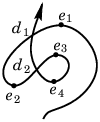
Local extrema of the composition of and the projection to the -axis are called extremal points. At an extremal point the curve goes either in a clockwise or a counter-clockwise direction, see Figure 8. Let be in the counter-clockwise case and otherwise. In Figure 9, and .
The preimage of an extremal point of divides into two rays. The curve is decomposed into the halves which are the images of these rays. Denote by and , respectively, the index of with respect to the half of approaching from the right and left, respectively. Put where the summations run over all extremal points of . For the curve in Figure 9, and .
Theorem 4.C.
Let be a long knot whose projection to -plane and -axis are generic. Let be the Gauss diagram corresponding to the projection to the -plane. Then
| (11) |
| (12) |
| (13) |
Here , , and are the characteristics of the
projection of defined in Section 4.8, and is the sum over all subdiagrams
of isomorphic to either
![[Uncaptioned image]](9903158v1/xleft.png) , or
, or
![[Uncaptioned image]](9903158v1/xright.png) , where ,
are the chords of the subdiagram, see Section 1.2.
, where ,
are the chords of the subdiagram, see Section 1.2.
Theorem 4.C is stated for a diagram of a long knot. However, it can be modified appropriately giving rise to a formulation similar to Corollary 4.B.
For a generic immersion put , where runs over extremal points of and is the index of with respect to . The preimage of a double point of divides into two arcs. The curve is decomposed into the halves which are the images of these arcs. One of them turns at in the clockwise direction, the other one turns counter-clockwise. Denote by and , respectively, the index of with respect to the former and latter, respectively. Put , where runs over all double points of .
Corollary 4.D.
Let be a knot whose projection to -plane and -axis are generic. Let be the Gauss diagram corresponding to the projection to the -plane. Then
| (14) |
4.11. Digression: Relation to Arnold’s Invariants of Plane Curves
Notice that in all the formulas of this Section there is a part depending only on the knot projection. Moreover the rest of the formula is common for all of the formulas: Thus the parts of the formulas depending only on the plane curve represent the same characteristic of the plane curve. Denote it by .
It is easy to identify it with a linear combination of invariants and of a generic immersion introduced by Arnold [2].
Indeed, consider an ascending diagram of the unknot with the given planar projection. Since of unknot is ,
where is the corresponding Gauss diagram of the unknot. The latter coincides with the Gauss diagram formula for proved in [20].
coincides with the invariant which was extracted by Lin and Wang [15] from Bar-Natan’s integral formula [4] representing .
All the formulas for described above in this section can be considered as formulas for .
5. New Configuration Spaces and Formulae
5.1. A Digression on the Degree of a Map
The two classical methods for calculating the degree of a map discussed in Section 3.6 above, admit the following common generalization. Let and be oriented smooth closed manifolds of dimension . Let be connected and be its oriented smooth closed connected submanifold. Let be a differentiable map transversal to . The orientations of and define an orientation of the normal bundle of in . Because of transversality, is a smooth submanifold of . The normal bundle of is naturally isomorphic to the pull back of the normal bundle of and gets oriented. This orientation together with the orientation of defines an orientation of . Therefore, both and are oriented smooth closed manifolds of the same dimension and the map defined by has a well-defined degree. Obviously, this degree coincides with the degree of .
It can be calculated by both of the classical methods. However the first method gives the expression for the degree literally coinciding with the one obtained by this method applied to the original map. The second method gives a new expression for the degree. In the case when is a point, this coincides with the expression obtained by the first method. In the case , this coincides with the expression provided by the second method applied to . So, this is indeed a generalization of both methods.
There are obvious generalizations of this observation. First, can be a stratified pseudomanifold. Then the transversality condition is formulated as follows: the restrictions of to strata of dimension are transversal to . Second, a relative situation can be considered: and are replaced by pairs and with and where . Then the degree of a map is equal to the degree of the induced map
Despite of apparent simplicity of this trick, it allows us to obtain several new geometrically interesting presentations of . We apply it to the map and various . However, this scheme is not easy to follow. The first difficulty is related to the transversality condition. The map has to be transversal to on each stratum of (of all the dimensions). The number of strata is rather large. Moreover, in all the interesting cases there are strata on which the transversality condition is not satisfied. Another difficulty is that in the most interesting cases . This problem is similar to the one we encountered in Section 4. There we stepped back to a generic situation and then passed to limit. Here we can follow the same pattern, but prefer to consider the geometry related to in detail.
The initial point of this consideration is still the structure of . However now we first take the intersection of with the union of all 6-dimensional strata of . Denote it by . Then take the closure of in . Denote the resulting space by . It is smaller and simpler than : even some high-dimensional strata of do not show up. This does not mean that we start over again from scratch. We use the way how the high-dimensional strata of are attached to each other. Furthermore, since on these strata is transversal to , we can define the orientations using the scheme above. Calculation of the degree is reduced to the case studied above via consideration of the preimage of a regular value.
5.2. Locking the Free Point on a Chord
Choose for the diagonal
One can check that for a knot in general position the restriction of to each 6-dimensional stratum of is transversal to . Let us identify with by and denote by the map induced by .
is a four-dimensional pseudo-manifold. Its four-dimensional strata are the components of . The components originated from can be identified with subspaces of obtained by locking the free point on a line connecting and with . These subspaces are even closer to the initial motivation for introducing auxiliary strata, see Figure 4.
The strata related to look as follows. For , denote by the subspace of defined by the condition
- (1)
lies on the line connecting and between them, if ,
- (2)
lies on the line connecting and outside , if ,
- (3)
lies on the line connecting and between them, if .
In the obvious sense, these spaces are associated with the diagrams shown in Figure 10.

Denote by the closure of in .
The intersection of with can be identified with:
- (1)
if or ;
- (2)
if or
- (3)
if or .
Under these identifications, turns into the maps extending the ones defined by the following formulas on with respectively:
- (1)
;
- (2)
;
- (3)
.
Four other four-dimensional strata of can be identified with . These strata are the intersections of with , for . On two of these strata is identified with and on two others, with followed by the permutation of the factors in .
For the two remaining (i.e., and ), the intersections of with can be naturally identified with the product , where
| (15) |
Under this identification, turns to , where
The identifications which have been made in the construction of reduce the boundary of in . The remaining 3-dimensional strata of the boundary coincide with the 3-dimensional strata of . Denote the closure of these boundary strata by .
Observe that each 4-dimensional stratum of described above appears twice, with the same mapping to . This happens because is defined by and the permutation , which acts in , commutes with , which acts in . Therefore, we can quotient out by the induced involution. The resulting space has six 4-dimensional strata: , , , two copies of , and the stratum .
Denote by the set
It is a bouquet of three copies of . Note that has codimension in , in contrast to , which has codimension in . A straightforward modification of Theorem 3.A looks as follows.
Theorem 5.A.
The space has a well-defined fundamental class . The map induces homomorphism
which maps to .∎
5.3. Configurations of Parallel Arrows
Aa part of coincides with , which is mapped to by . This part of differs in its nature from the rest of the main strata. It turns out that this part can be splitted out.
Observe that is is the preimage of the diagonal under the map . The orientation of (defined by the orientation of ) can be computed as described in Section 5.1. To a generic point , there correspond the projection along and two crossings of this projection: and . At such a point, one can take as local coordinates and . The local degree of with respect to the orientation defined by the coordinate system is the sign of . The local degree of at this point is the product of this sign and . Hence the orientation of differs from the orientation defined by the coordinate system by .
Denote by the closure of in and denote by the extension of to . The 1-strata of , whose images under do not coincide with , are , . There are embeddings
Let be the quotient space of obtained by identification of with via these embeddings. It is easy to check that defines a map . Denote this map by the same symbol .
Theorem 5.B.
has a well-defined fundamental class . The map induces homomorphism , which maps to .
Proof.
The local degree of at a generic point is . Summing up the local degrees at all points of the preimage of some regular value, we obtain the right hand side of (1). ∎
Let us return to the space of Section 5.2. Remove from and sue the edge of the cut by and . Denote the result by (superindex stands for “line” alluding to locking the free point on a line). Denote by the map defined by . Denote by the subspace of obtained from . Combining Theorems 5.A and 5.B, we get the following theorem.
Theorem 5.C.
The space has a well-defined fundamental class . The map induces homomorphism , which maps to .∎
5.4. Application: New Integral Formula
Theorem 5.C gives rise to an integral formula for by choosing the standard volume form on , pulling it back by and integrating over . Put
Recall that for a knot we denote by the space of 3-tuples of points ordered in the natural way defined by the orientation of with .
Corollary 5.D.
| (16) |
∎
5.5. Slicing by Parallel Planes
Now choose for the 3-torus
For a knot in general position the restriction of to each 6-dimensional stratum of is transversal to . Denote by the map induced by . Now is a 3-dimensional pseudo-manifold, which has twelve 3-dimensional strata.
Six of them, which are with , can be identified with , where
In other words, is the space whose points are 4-tuples of points on the knot such that each of the pairs and lies in a plane orthogonal to , see Figure 11.

The other six strata, which are with , can be identified with , where
The space consists of 4-tuples of points lying in the same plane orthogonal to such that , and belong to . See Figure 11.
As above in Section 5.2, 2-dimensional strata of the boundary of coincide with the 2-dimensional strata of . They are contained in the closure of . A point of these strata can be interpreted as a triple of points contained in the same plane orthogonal to , which is tangent to the knot at one of these points and intersects the knot in one of the other two points. Such a configuration appears as a limit of 4-tuples belonging to when two of the points on the knot collide.
Denote the closure of these boundary strata by .
Denote by the set
Applying now the scheme described in Section 5.1, we obtain the following theorem.
Theorem 5.E.
has a well-defined fundamental class . The map induces homomorphism , which maps to .∎
5.6. Yet Another Integral Formula
Theorem 5.E gives rise to an integral formula for by choosing the standard volume form on , pulling it back by and integrating over . Put
This is the normalized length form on the circle in the -plane.
For fixed , a 4-tuple of points on -plane is called a -slice if there exists such that and have -coordinates equal to , and have -coordinates equal to , and the projection of to -plane is . Denote by the number of ’s such that the projection to -axis of a positively oriented tangent vector to the knot is negative. For a fixed , a triple of points on -plane is called a -slice if there exists such that has -coordinate equal to and the projection to -plane is . Denote by the number of ’s with such that the projection to -axis of a positively oriented tangent vector to the knot is negative.
Corollary 5.F.
| (17) |
∎
Remark 5.G.
The first integral is similar to the integral in the Kontsevich formula for , see [12] and [4]. However, in our formula we have instead of only the imaginary part of . Thus the contribution of the real part of to the Kontsevich formula is replaced by the second integral. A similar relation between the associators in non-associative tangles and the contribution of already appeared in Section 4.7–4.9. This may shed light onto yet non-understood relation between the integral formulas of Kontsevich [12], [4] and Bott-Taubes [6].
References
- [1] S. Akbulut and J. McCarthy, Casson’s invariant for oriented homology 3-spheres — an exposition, Princeton Math. Notes 36, Princeton University Press, 1990.
- [2] V.I.Arnold, Topological invariants of plane curves and caustics, University lecture series (Providence RI) 5 (1994)
- [3] S.Axelrod and I.M.Singer, Chern-Simons Perturbatin Theory, in Proceedings of the XXth DGM Conference, edited by S.Catto and A. Rocha (World Scientific, Singapore, 1992), 3–45; Chern-Simons Perturbation, II, J. Diff. Geom. 39 (1994) 173–213.
- [4] D. Bar-Natan, On the Vassiliev knot invariants, Topology 34 (1995) 423–472.
- [5] D. Bar-Natan, Non-associative tangles, in Geometric topology (proceedings of the Georgia international topology conference), (W. H. Kazez, ed.), 139–183, AMS and International Press, Providence, 1997.
- [6] R. Bott, C. Taubes, On the self-linking of knots, J. Math. Phys. 35 (1994), 5247–5287.
- [7] P. Cartier, Construction combinatoire des invariants de Vassiliev-Kontsevich des noeuds, C. R. Acad. Sci. Paris 316 (1993), 1205–1210.
- [8] W. Fulton, R. MacPherson, A Compactification of Configuration Spaces, Ann. Math. 139 (1994), 183–225.
- [9] P. Gilmer, A method for computing the Arf invariants for links, Quantum Topology, Series on Knots and Everything Vol. 3, ed. L. Kauffman and R. Baadhio, World Sci., Singapore, 1993, 174–181.
- [10] M. Goussarov, M. Polyak, O. Viro, Finite Type Invariants of Classical and Virtual Knots, preprint math.GT/9810073.
- [11] Louis H. Kauffman, On Knots, Annals of Math. Studies 115, Princeton University Press (1987).
- [12] M. Kontsevich, Vassiliev’s knot invariants, Adv. Sov. Math. 16 (1993), 137–150.
- [13] Jean Lannes, Sur les invariants de Vassiliev de degré infeŕieur ou égal à 3, Enseign. Math. (2) 39 (1993) no. 3-4, 295–316.
- [14] Jean Lannes, Sur l’invariant de Kervaire des noueds classiques, Comment. Math Helvetici, 60 (1985) 179–192.
- [15] Xiao-Song Lin and Zhenghan Wang, Integral geometry of plane curves and knot invariants, J. Diff. Geom. 44 (1996), no. 1, 74–95.
- [16] Ka Yi Ng, Groups of ribbon knots, Topology 37 (1998) 441–458.
- [17] S. Piunikhin, Combinatorial expressions for universal Vassiliev link invariant, Comm. Math. Phys. 168-1 1–22.
- [18] Sylvain Poirier, Rationality results for the configuration space integral of knots, preprint math.GT/9901028.
- [19] Michael Polyak and Oleg Viro, Gauss Diagram Formulas for Vassiliev invariants, Int. Math. Research Notices, 11 (1994) 445–453.
- [20] Michael Polyak, Invariants of curves and fronts via Gauss diagrams, Topology 37 (1998) 989–1009.
- [21] Michael Polyak, On the algebra of arrow diagrams, preprint http://www.math.tau.ac.il/˜ polyak/.
- [22] Dale Rolfsen, Knots and links, Publish or Perish, Inc., 1990.
- [23] D. Thurston, Integral expressions for the Vassiliev knot invariants, Harvard University senior thesis, April 1995.
- [24] V.A.Vassiliev, Cohomology of knot spaces, Theory of singularities and its applications (Providence) (V.I.Arnold, ed.) AMS, Providence, 1990.