One-skeleta, Betti numbers and equivariant cohomologyThanks: * Supported by NSF grant DMS 890771.

V. Guillemin¹¹footnotemark: 1 * Address: Department of Mathematics, MIT, Cambridge, MA 02139 Email address: vwg@@math.mit.edu and C. Zara Address: Department of Mathematics, MIT, Cambridge, MA 02139 Email address: czara@math.mit.edu

Abstract.

The one-skeleton of a $G$ -manifold $M$ is the set of points $p\in M$ where $\dim G_{p}\geq\dim G-1$ ; and $M$ is a GKM manifold if the dimension of this one-skeleton is 2. Goresky, Kottwitz and MacPherson show that for such a manifold this one-skeleton has the structure of a “labeled” graph, $(\Gamma,\alpha)$ , and that the equivariant cohomology ring of $M$ is isomorphic to the “cohomology ring” of this graph. Hence, if $M$ is symplectic, one can show that this ring is a free module over the symmetric algebra ${\mathbb{S}}({\mathfrak{g}}^{*})$ , with $b_{2i}(\Gamma)$ generators in dimension $2i$ , $b_{2i}(\Gamma)$ being the “combinatorial” $2i$ -th Betti number of $\Gamma$ . In this article we show that this “topological” result is , in fact, a combinatorial result about graphs.

Introduction

Let $G$ be a commutative, compact, connected, $n$ -dimensional Lie group, ${\mathfrak{g}}$ its Lie algebra, $M$ a compact $2d$ -dimensional manifold and $\tau:G\times M\to M$ a faithful action of $G$ on $M$ . We say that $M$ is a GKM manifold if it has the following properties:

(1)

$M^{G}$ is finite.
(2)

$M$ possesses a $G$ -invariant almost-complex structure.
(3)

For every $p\in M^{G}$ , the weights

$\alpha_{i,p}\in{\mathfrak{g}}^{*}\,,\,i=1,\ldots,d\,,$ (0.1)

of the isotropy representation of $G$ on $T_{p}M$ are pairwise linearly independent.

There is an alternate way of formulating this third condition: Let $M$ be a $G$ -manifold which satisfies the first two conditions, and define the one-skeleton of $M$ to be the set of points, $p\in M$ with $\dim G_{p}\geq n-1$ . Then $M$ satisfies the third condition if and only if its one-skeleton consists of $G$ -invariant submanifolds which are fixed point free and $G$ -invariant embedded $2$ -spheres, each of which contains exactly two fixed points. Thus the combinatorial structure of this one-skeleton is that of a graph $\Gamma$ having the fixed points of $G$ as vertices and these $2$ -spheres as edges. As we will see in the next section, $\Gamma$ is a regular graph: each vertex is the point of intersection of exactly $d$ edges. Moreover, the action of $G$ on $M$ gives one a labeling of the oriented edges of $\Gamma$ by one-dimensional representations of $G$ . Namely, to each oriented edge, $e$ , one can assign the isotropy representation, $\chi_{e}$ , of $G$ on the tangent space at the “north pole” of the corresponding $S^{2}$ , the “north pole” corresponding to the initial vertex of $e$ . Thus one has a map

\alpha:E_{\Gamma}\to{\mathfrak{g}}^{*}

from the set of oriented edges of $\Gamma$ to ${\mathfrak{g}}^{*}$ , which assigns to each oriented edge, $e$ , the weight, $\alpha_{e}$ , of the representation $\chi_{e}$ . We will refer to the pair $(\Gamma,\alpha)$ as the GKM one-skeleton associated to $M$ .

A beautiful result of Goresky-Kottwitz-MacPherson asserts that if $M$ is equivariantly formal, the equivariant cohomology ring, $H_{G}(M)$ , can be reconstructed from the GKM one-skeleton. More explicitly, let $V_{\Gamma}$ be the vertices of $\Gamma$ and $H(\Gamma,\alpha)$ the set of all maps, $f:V_{\Gamma}\to{\mathbb{S}}({\mathfrak{g}}^{*})$ , which satisfy the compatibility condition

f(p)-f(q)=0\mod{\alpha_{e}}

(0.2)

for every pair of vertices $p$ and $q$ , and every edge, $e$ , joining $p$ and $q$ . Then the GKM theorem asserts

H_{G}(M)\simeq H(\Gamma,\alpha).

(0.3)

One interesting implication of this theorem is that one can prove, by topology, combinatorial results about $H(\Gamma,\alpha)$ . For instance, suppose that the action, $\tau$ , of $G$ on $M$ is Hamiltonian. Then, by a theorem of Kirwan, $M$ is equivariantly formal; so the GKM theorem applies to $M$ . Moreover, from the constant map,, $\gamma:M\to pt$ , one gets a map, $\gamma^{*}:H_{G}(pt)\to H_{G}(M)$ , and since $H_{G}(pt)={\mathbb{S}}({\mathfrak{g}}^{*})$ , this map makes $H_{G}(M)$ into an ${\mathbb{S}}({\mathfrak{g}}^{*})$ -module. If $\tau$ is Hamiltonian, Kirwan proves that $H_{G}(M)$ is a free ${\mathbb{S}}({\mathfrak{g}}^{*})$ -module with $b_{2i}(M)$ generators in dimension $2i$ , $b_{2i}(M)$ being the $2i$ -th Betti number of $M$ . In addition, using Morse theory, one can compute these Betti numbers directly from the GKM one-skeleton, $(\Gamma,\alpha)$ , as follows: Fix $\xi\in{\mathfrak{g}}$ with $\alpha_{e}(\xi)\neq 0$ for all $e\in E_{\Gamma}$ and let $b_{2i}(\Gamma)$ be the number of vertices, $p$ , for which there are exactly $i$ oriented edges, $e$ , with initial vertex $p$ , such that $\alpha_{e}(\xi)<0$ . Then

b_{2i}(\Gamma)=b_{2i}(M).

(0.4)

Thus, by topology, one proves

Theorem 0.0.1.

$H(\Gamma,\alpha)$ is a free ${\mathbb{S}}({\mathfrak{g}}^{*})$ -module. Moreover

H(\Gamma,\alpha)\otimes_{{\mathbb{S}}({\mathfrak{g}}^{*})}{\mathbb{C}}

(0.5)

is a finite dimensional graded ring, its $2i$ -th graded component being of dimension $b_{2i}(\Gamma)$ .

There are a number of other theorems about the structure of $H(\Gamma,\alpha)$ which can be proved “by topology”. For instance, using equivariant Morse theory, one can write down a canonical set of generators of $H(\Gamma,\alpha)$ , and if $\tau$ is Hamiltonian, one can, by methods of Kirwan ([Ki]) prove a number of interesting facts about subrings and quotient rings of $H(\Gamma,\alpha)$ . (See, for instance, [TW1].)

The question we want to explore in this paper is: Can one prove these “topological” results about $H(\Gamma,\alpha)$ purely by combinatorial methods ? In other words, are these theorems combinatorial theorems about graphs in disguise ? Two types of GKM manifolds for which this question has a positive answer are toric varieties and flag varieties. For toric varieties $H_{G}(M)$ is the Stanley-Reisner ring of the moment polytope of $M$ , and for flag varieties, $H_{G}(M)$ is the ring of “double Schubert polynomials”; and, in these cases, the theorems above follow from combinatorial theorems about poset cohomology, root systems, Hecke algebras et al. (See [Bi], [BH], [Fu1], [Fu2], [Hu], [LS], [St]) Therefore the question above is part of a more open-ended question: Are there analogues of some of these combinatorial theorems for GKM manifolds in general ?

The interplay between graphs and GKM manifolds may have some interesting applications in graph theory per se. We will describe one example of such an application: Let $\Delta$ be a convex polytope in ${\mathbb{R}}^{n}$ and let $\Gamma$ be its one-skeleton, i.e. the graph consisting of the vertices and edges of $\Delta$ . Then, just as above, the oriented edges of $\Gamma$ have a natural labeling: to each oriented edge, $e$ , one can assign the edge vector, $\alpha_{e}=q-p$ , $p$ and $q$ being the initial and the terminal vertices of $e$ . In analogy with the case of GKM manifolds, we will call the pair $(\Gamma,\alpha)$ the GKM one-skeleton of $\Delta$ . A problem of interest to combinatorists (see, for instance, [CW]) is how to deform $\Delta$ so that the directions of its edges are unchanged. In particular, how many such deformations are there ? GKM theory suggests an answer: If $\Delta$ is a simple polytope and its edge directions are rational, it is the moment polytope of a toric variety, $M$ ; and the number of ways in which one can deform $\Delta$ without changing its edge directions is equal, by Delzant’s theorem ([Del]), to the number of ways in which one can deform the symplectic structure of $M$ , i.e. is equal to $\dim H^{2}(M)$ , or, alternatively, by (0.3), is equal to $b_{2}(\Gamma)$ . We will show in section 3.2 that this result is true not just for simple polytopes but for all convex polytopes which have the following “edge-reflecting” property: If two vertices, $p$ and $q$ , of $\Gamma$ are joined by an edge, $e$ , then for every edge, $e^{\prime}$ , containing $p$ , there exists a unique edge, $e^{\prime\prime}$ , containing $q$ , such that, $e^{\prime}$ and $e^{\prime\prime}$ are coplanar. (This is a joint result with Ethan Bolker.)

This article consists of three chapters. In chapter one we review the theory of GKM manifolds and describe how to translate geometric properties of these manifolds into combinatorial properties of their associated GKM graphs. In chapter two we define an abstract one-skeleton to be a labeled graph $(\Gamma,\alpha)$ for which $\alpha$ satisfies certain simple axioms (axiomatizing properties of the GKM-skeleta discussed in chapter one.) We then define the cohomology ring, $H(\Gamma,\alpha)$ , to be, as above, the set of all maps, $f:V_{\Gamma}\to{\mathbb{S}}({\mathfrak{g}}^{*})$ which satisfy the compatibility conditions (0.3) and prove that this ring is a free ${\mathbb{S}}({\mathfrak{g}}^{*})$ -module with $b_{2i}(\Gamma)$ generators in dimension $2i$ . (Involved in the proof of this theorem are the graph-theoretical analogues of two basic theorems in equivariant symplectic geometry: the Kirwan surjectivity theorem and the “blow-up-blow-down” theorem of Brion-Procesi-Guillemin-Sternberg-Godinho. Both these theorems have to do with the concept of symplectic reduction, and a large part of chapter two will be concerned with defining this concept in the context of abstract one-skeleta.)

Chapter three contains a number of applications. One of these is the theorem about edge-reflecting polytopes which we described above. Another is a “realization” theorem for abstract GKM-skeleta. This asserts that an abstract one-skeleton $(\Gamma,\alpha)$ is the GKM one-skeleton of a GKM manifold if and only is $\alpha$ satisfies certain integrality conditions. This is a joint result with Viktor Ginzburg, Yael Karshon and Sue Tolman and is closely related to the realization theorem proved by them in [GKT].

A third application has to do with the theory of Schubert polynomials. In Section 3.3 we show that, for the Grassmannian, $Gr^{k}({\mathbb{C}}^{n})$ , the canonical generators of $H(\Gamma,\alpha)$ predicted by our theory have an alternative description in terms of the Hecke algebra of divided difference operators and thus can be identified with the “double Schubert polynomials” of [Bi]. (Together with Tara Holm we have generalized this to all partial flag varieties; for details, see [GHZ].)

We would like to express our thanks to several of our colleagues for helping us to understand some of the key motivating examples in this subject: David Vogan for furnishing us with an enlightening example of a GKM action of $T^{2}$ on $S^{6}$ , Yael Karshon, Viktor Ginzburg and Sue Tolman for furnishing us with an equally enlightening example of a GKM action of $T^{2}$ on the $n$ -fold equivariant ramified cover of $S^{2}\times S^{2}$ , Mark Goresky for pointing out to us the connection between the GKM theory of toric varieties and Stanley-Reisner theory, Werner Ballmann for making us aware of the fact that, for the Grassmannian, GKM theory reduces to studying an object which graph theorists call the Johnson graph, Sara Billey for helping us to understand the tie-in between our theory of Thom classes for this graph and the standard Schubert calculus, Rebecca Goldin and Tara Holm for helping us work out the details of this example (in sections 1.11 and 3.3) and Ethan Bolker for his beautiful observation (see section 1.3, Theorem 1.3.1) that the Betti numbers of a GKM one-skeleton are well-defined, independent of the choice of an admissible orientation. Last, but not least, we would like to thank the referee of this paper for a superb refereeing job.

1. GKM manifolds

1.1. The GKM one-skeleton

For each of the weights $\alpha_{i,p}$ on the list (0.1) let $H_{i}$ be the identity component of the kernel of the map

\exp{\xi}\in G\longrightarrow\exp{(\sqrt{-1}\alpha_{i,p}(\xi))}

and let $X_{i}$ be the connected component of $M^{H_{i}}$ containing $p$ .

Theorem 1.1.1.

$X_{i}$ is diffeomorphic to $S^{2}$ and the action of $G$ on $X_{i}$ is diffeomorphic to the standard rotation action of the circle $G/H_{i}$ on $S^{2}$ .

Proof.

Consider the decomposition

T_{p}M=\bigoplus T_{p}^{\alpha_{i,p}}

of $T_{p}M$ into 2-dimensional weight spaces. Our assumption that the weights (0.1) are pairwise linear independent imply that

T_{p}X_{i}=T_{p}^{\alpha_{i,p}}

and hence that $X_{i}$ is two-dimensional. Since the only oriented two-manifold with faithful $S^{1}$ actions are $S^{2}$ and $T^{2}$ , $X_{i}$ has to be one of them. However, the action of $S^{1}$ on $T^{2}$ is fixed point free, so $X_{i}$ is diffeomorphic to $S^{2}$ . Finally, the fact that the action of $S^{1}$ is the standard $S^{1}$ action is standard. ∎

Thus $p$ is the point of intersection of $d$ embedded $G$ -invariant 2-spheres. These can be represented graphically as in the figure below:

Refer to caption — Figure 1. A vertex of the GKM graph

Each of these 2-spheres joins $p$ to another fixed point $q_{i}$ and each $q_{i}$ is in turn the point of intersection of $d$ 2-spheres. One of these is $X_{i}$ and rejoins $q_{i}$ to $p$ , but the others join $q_{i}$ to other fixed points, and at these points we can repeat the construction. We will define the GKM graph $\Gamma$ to be the graph we obtain by repeating this construction until we run out of fixed points.

This graph can be defined more intrinsically as follows: the vertices of $\Gamma$ correspond to the fixed points of $M$ , an edge, $e$ , of $\Gamma$ corresponds to a $G$ -invariant embedded two-sphere, $X_{e}$ , and joins the vertices that correspond to the two fixed points situated on $X_{e}$ . For an oriented edge $e$ , we will denote by $i(e)$ and $t(e)$ the initial and terminal vertices of $e$ . In addition, we will denote by $\bar{e}$ the edge $e$ with its orientation reversed. Thus $i(\bar{e})=t(e)$ and $i(e)=t(\bar{e})$ .

To keep track of the action of $G$ on this configuration of embedded $S^{2}$ ’s we will assign to each oriented edge $e$ the weight $\alpha_{e}$ of the isotropy representation of $G$ on $T_{i(e)}X_{e}$ . Denoting by $E_{\Gamma}$ the set of oriented edges of $E$ , this gives us a map

\alpha:E_{\Gamma}\to{\mathfrak{g}}^{*}

which we will call the axial function of $\Gamma$ . The pair $(\Gamma,\alpha)$ will be called the GKM one-skeleton associated to the GKM manifold $M$ .

Let $V_{\Gamma}$ be the set of vertices of $\Gamma$ and let

\pi:E_{\Gamma}\to V_{\Gamma}

be the fibration defined by $\pi(e)=i(e)$ . A connection on the bundle $(E_{\Gamma},V_{\Gamma},\pi)$ is, by definition, a recipe for transporting the fibers of $\pi$ along paths in $\Gamma$ . In particular, a canonical connection can be defined as follows. Let $e$ be an oriented edge of $\Gamma$ joining the vertex $p=i(e)$ to the vertex $p^{\prime}=t(e)$ and let $e_{i}$ and $e_{i}^{\prime}$ , for $i=1,..,d$ , be the “points” (i.e. oriented edges) on the fibers above $p$ and $p^{\prime}$ . By a theorem of Klyashko ([Kl]), the restriction to $X_{e}$ of the tangent bundle to $M$ splits equivariantly into a sum of line bundles

\bigoplus{\mathbb{L}}_{i},\qquad i=1,..,d

(1.1)

and one can relabel the $e_{i}$ ’s and $e_{i}^{\prime}$ ’s so that

({\mathbb{L}}_{i})_{p}=T_{p}X_{e_{i}}\quad\mbox{ and }\quad({\mathbb{L}}_{i})_{p^{\prime}}=T_{p^{\prime}}X_{e_{i}^{\prime}}

and from this one gets a canonical identification $e_{i}\longleftrightarrow e_{i}^{\prime},$ i.e. a canonical map

\theta_{e}:E_{p}\to E_{p^{\prime}},

$E_{p}$ being the fiber $\pi^{-1}(p)$ above $p$ and $E_{p^{\prime}}$ the fiber above $p^{\prime}$ .

Associated to the notion of connection is that of holonomy. Consider a connection, $\theta$ , on $\Gamma$ and fix $p\in V_{\Gamma}$ . For each loop, $\gamma$ , starting and ending at $p$ one gets a bijection, $\sigma_{\gamma}:E_{p}\to E_{p}$ , by composing the maps corresponding to the edges of $\gamma$ . Let $Hol(\Gamma,\theta,p)$ be the subgroup of the permutation group $\Sigma(E_{p})$ generated by the elements of the form $\sigma_{\gamma}$ for all loops $\gamma$ based at $p$ . If $p_{1}$ and $p_{2}$ can be connected by a path then the holonomy groups $Hol(\Gamma,\theta,p_{1})$ and $Hol(\Gamma,\theta,p_{2})$ are isomorphic by conjugacy; therefore we can define the holonomy group $Hol(\Gamma,\theta)$ as being the group, $Hol(\Gamma,\theta,p)$ , for any point $p$ . We will also say that $\theta$ has trivial holonomy if $Hol(\Gamma_{i},\theta)$ is trivial for each connected component $\Gamma_{i}$ of $\Gamma$ .

The following theorem lists some basic properties of the triple $(\Gamma,\alpha,\theta)$ .

Theorem 1.1.2.

(1)

For every $p\in V_{\Gamma}$ , the weights $\alpha_{e}$ , $e\in E_{p}$ , are pairwise linearly independent.
(2)

For every $e\in E_{\Gamma}$ , $(\theta_{e})^{-1}=\theta_{\bar{e}}$ .
(3)

$\theta_{e}$ maps $e$ to $\bar{e}$ .
(4)

$\alpha_{\bar{e}}=-\alpha_{e}$ .
(5)

Let $p=i(e)$ , $p^{\prime}=t(e)$ and let $e_{i}\leftrightarrow e_{i}^{\prime}$ , $i=1,..,d$ be the map of $E_{p}$ onto $E_{p^{\prime}}$ defining $\theta_{e}$ . Then

$\alpha_{e_{i}^{\prime}}=\alpha_{e_{i}}+c\alpha_{e}$ (1.2)

for some constant $c=c_{i,e}$ depending on $i$ and $e$ .

Proof.

The first four assertions are obvious. To prove the last one, let $H$ be the identity component of the kernel of the map

\exp{\xi}\in G\longrightarrow\exp{(\sqrt{-1}\alpha_{e}(\xi))}.

Each point of $X_{e}$ is an $H$ -fixed point, so for each $x\in X_{e}$ one has an isotropy representation of $H$ on $T_{x}M$ . The weights of this representation are independent of $x$ , so they are the same at $p$ and $p^{\prime}$ . ∎

Remark.

It is easy to see that the constants $c_{i,e}$ in (1.2) are integers. In fact, let $c({\mathbb{L}}_{i})$ be the Chern class of the line bundle ${\mathbb{L}}_{i}$ in (1.1). By the Atiyah-Bott-Berline-Vergne localization theorem, the integral of $c({\mathbb{L}}_{i})$ over $X_{e}$ is

c_{i,e}=\frac{\alpha_{e_{i}^{\prime}}-\alpha_{e_{i}}}{\alpha_{e}}\quad;

(1.3)

hence $c_{i,e}$ is the Chern number of ${\mathbb{L}}_{i}$ , and so, in particular, an integer.

1.2. GKM theory for orbifolds

By “orbifolds” we will mean orbifolds having a presentation of the form $M=X/K$ , $K$ being a torus and $X$ being a manifold on which $K$ acts in a faithful, locally free fashion. GKM theory for such orbifolds is essentially the same as GKM theory for manifolds, the major difference being that the $S^{2}$ ’s corresponding to the edges of the graph $\Gamma$ may now be orbifold $S^{2}$ ’s, that is are either tear-drops or footballs.

One consequence of this is that the axiomatic properties of the axial function $\alpha$ are slightly more complicated. For each point $p=xK\in M$ , with $x\in X$ , let $m_{p}=\#K_{x}$ . Then, if $e\in E_{\Gamma}$ , item 4 in Theorem 1.1.2 has to be replaced by

m_{i(\bar{e})}\alpha_{\bar{e}}=-m_{i(e)}\alpha_{e};

(1.4)

however, the other properties of $\alpha$ described in Theorem 1.1.2 are still true as stated.

Example 1.2.1.

Let $M$ be the football of type $(m,n)$ , that is the quotient:

({\mathbb{C}}^{2}-0)/\sim,

where

(z_{1},z_{2})\sim(\lambda^{m}z_{1},\lambda^{n}z_{2})

with $\lambda\in{\mathbb{C}}-0$ and $m,n$ relatively prime positive integers. Let $S^{1}$ act on $M$ by the action

e^{i\theta}[z_{1}:z_{2}]=[e^{i\theta}z_{1}:e^{i\theta}z_{2}].

The fixed points of this action are $p=[0:1]$ and $q=[1:0]$ , and a coordinate system centered at $p$ is given by

z\in{\mathbb{C}}\to[z:1].

In this coordinate system $z\sim\omega_{n}^{k}z$ , $\omega_{n}$ being a primitive $n$ -th root of unity, so, in particular, $m_{p}=n$ . The action of $S^{1}$ in this coordinate system is given by

e^{i\theta}[z:1]=[e^{i\theta}z:e^{i\theta}]=[e^{i\frac{n-m}{n}\theta}z:1],

so the weight of the isotropy representation of $S^{1}$ on $T_{p}M$ is $\alpha_{p}=\frac{n-m}{n}$ ; similarly $m_{q}=m$ and $\alpha_{q}=\frac{m-n}{m}$ so that

m_{p}\alpha_{p}=-m_{q}\alpha_{q},

in confirmation of (1.4).

Notice, by the way, that the character associated with this weight, $e^{i\frac{n-m}{n}\theta}$ , is taking values not in $S^{1}$ but in $S^{1}/\{\omega_{n}^{k}\}$ . This is, of course, consistent with the fact that the linear action of $S^{1}$ on the coordinate system above is only an action modulo the identification $z\sim\omega_{n}^{k}z$ .

1.3. Combinatorial Betti numbers

Let $M$ be a GKM manifold and $(\Gamma,\alpha)$ its GKM one-skeleton; we say that $\xi\in{\mathfrak{g}}$ is a polarizing vector if $\alpha_{e}(\xi)\neq 0$ for all $e\in E_{\Gamma}$ , and we denote by ${\mathcal{P}}$ the set of polarizing vectors, i.e.

{\mathcal{P}}=\{\xi\in{\mathfrak{g}};\alpha_{e}(\xi)\neq 0\mbox{ for all }e\in E_{\Gamma}\}.

(1.5)

For a fixed $\xi\in{\mathcal{P}}$ define the index $\sigma_{p}$ of a vertex $p\in V_{\Gamma}$ to be the number of edges $e\in E_{p}$ with $\alpha_{e}(\xi)<0$ . This definition clearly depends on the choice of $\xi$ . Let

b_{2i}(\Gamma)=\#\{p;\sigma_{p}=i\}.

(1.6)

We claim that this definition doesn’t depend on $\xi$ , in spite of the fact that $\sigma_{p}$ does, and we will call $b_{2i}(\Gamma)$ the (combinatorial) $2i$ -th Betti number of $\Gamma$ .

Theorem 1.3.1.

$b_{2i}(\Gamma)$ doesn’t depend on $\xi$ ; it is a combinatorial invariant of $(\Gamma,\alpha)$ .

Proof.

Let ${\mathcal{P}}_{i},\;i=1,...,N$ , be the connected components of ${\mathcal{P}}$ and consider an $(n-1)$ -dimensional wall separating two adjacent ${\mathcal{P}}_{i}$ ’s. This wall is defined by an equation of the form

\alpha_{e}(\xi)=0

(1.7)

for some $e\in E_{\Gamma}$ . Let $p=i(e)$ , $q=t(e)$ , and let’s compute the changes in $\sigma_{p}$ and $\sigma_{q}$ as $\xi$ passes through this wall: Let $E_{p}=\{e_{i},\;i=1,...,d\}$ and $E_{q}=\{e^{\prime}_{i},\;i=1,...,d\}$ (with $e_{d}=e$ and $e^{\prime}_{d}=\bar{e}$ ). By item 5 of Theorem 1.1.2 we can order the $e_{i}$ ’s so that, for $i\leq d-1$ ,

\alpha_{e_{i}}=\alpha_{e^{\prime}_{i}}+c_{i}\alpha_{e}\;.

From item 1 of Theorem 1.1.2 it follows that for every $i=1,...,d-1$ ,

\mbox{dim}\,(\,\mbox{ker}\,\alpha_{e}\cap\mbox{ ker}\,\alpha_{e_{i}})=n-2

and therefore there exists $\xi_{0}$ such that $\alpha_{e}(\xi_{0})=0$ but $\alpha_{e_{i}}(\xi_{0})\neq 0\neq\alpha_{e^{\prime}_{i}}(\xi_{0})$ , for all $i=1,...,d-1$ .

Thus there exists a neighborhood $U$ of $\xi_{0}$ in ${\mathfrak{g}}$ such that for $i=1,...,d-1$ and $\xi\in U$ , $\alpha_{e_{i}}(\xi)$ and $\alpha_{e^{\prime}_{i}}(\xi)$ have the same sign, and this common sign doesn’t depend on $\xi\in U$ . Such a neighborhood will intersect both regions created by the wall (1.7). Now suppose that $\xi\in U$ and that $r$ of the numbers $\alpha_{e_{i}}(\xi),\;i=1,...,d-1,$ are negative. Since $\alpha_{\bar{e}}(\xi)=-\alpha_{e}(\xi)$ , it follows that for $\alpha_{e}(\xi)$ positive

\sigma_{p}=r\quad\mbox{ and }\quad\sigma_{q}=r+1

and for $\alpha_{e}(\xi)$ negative

\sigma_{p}=r+1\quad\mbox{ and }\quad\sigma_{q}=r.

In either case, as $\xi$ passes through the wall (1.7), the Betti numbers don’t change. ∎

Remark.

When we change $\xi$ to $-\xi$ , a vertex with index $k$ will now have index $d-k$ , where $d$ is the valence of $\Gamma$ . Since the Betti numbers don’t depend on $\xi$ it follows that

b_{2(d-k)}=b_{2k},\qquad\forall\;k=0,..,d.

(1.8)

We will show in section 1.9 that these combinatorial Betti numbers may not be, in general, equal to the Betti numbers of $M$ . An important exception, however, is the following:

Theorem 1.3.2.

If the action, $\tau$ , of $G$ on $M$ is Hamiltonian then $b_{2i}(\Gamma)=b_{2i}(M).$

Proof.

For $\xi\in{\mathcal{P}}$ , the vector field $\xi_{M}$ is Hamiltonian and its Hamiltonian function, $f$ , is a Morse function whose critical points are the fixed points of $\tau$ . Moreover, the index of a critical point, $p$ , is just $2\sigma_{p}$ , so the number of critical points of index $2i$ is $b_{2i}(\Gamma)$ ; for more details see [At]. ∎

Remark.

In the Hamiltonian case, the relation (1.8) is a direct consequence of Theorem (1.3.2) and Poincare duality.

1.4. Hamiltonian GKM-skeleta

We will discuss in this section a few graph theoretic pathologies which can’t occur if $(\Gamma,\alpha)$ is the GKM one-skeleton of a Hamiltonian $G$ -manifold. As in the previous section, fix a vector $\xi\in{\mathcal{P}}$ . For an unoriented edge $e$ , of $\Gamma$ , let $e^{+}\in E_{\Gamma}$ be the edge $e$ , oriented such that $\alpha_{e^{+}}(\xi)>0$ and let $e^{-}\in E_{\Gamma}$ be the edge $e$ with the opposite orientation. We are thus defining an orientation, $o_{\xi}$ (which we will call the $\xi$ -orientation), of the edges of $\Gamma$ , and it is clear that this orientation depends only on the connected component of ${\mathcal{P}}$ in which $\xi$ sits. On the other hand it is clear that different components will give rise to different orientations. (For instance, replacing $\xi$ with $-\xi$ reverses all the orientations.) For an oriented edge $e$ , let $e_{0}$ be the same edge, but unoriented; we will say that $e$ points upward if $e=e_{0}^{+}$ and that $e$ points downward if $\bar{e}=e_{0}^{+}$ . We will say that $(\Gamma,\alpha)$ is $\xi$ -acyclic if the oriented graph $(\Gamma,o_{\xi})$ has no cycles and that $(\Gamma,\alpha)$ satisfies the no-cycle condition if it is $\xi$ -acyclic for at least one $\xi$ .

Definition 1.4.1.

Given $\xi\in{\mathcal{P}}$ , a function $f:V_{\Gamma}\to{\mathbb{R}}$ is called $\xi$ -compatible if, for every edge, $e$ , of $\Gamma$ , $f(t(e^{+}))>f(i(e^{+}))$ .

If $f$ is injective and $\xi$ -compatible, the orientation, $o_{\xi}$ , of $\Gamma$ associated with $\xi$ can’t have cycles since $f$ has to be strictly increasing along any oriented path. The converse is also true:

Theorem 1.4.1.

If $(\Gamma,\alpha)$ is a $\xi$ -acyclic GKM one-skeleton then there exists an injective function, $f:V_{\Gamma}\to{\mathbb{R}}$ , which is $\xi$ -compatible.

Proof.

For a vertex $p$ , define $f_{0}(p)$ to be the length of the longest oriented path with terminal vertex at $p$ . Then $f_{0}$ is $\xi$ -compatible and takes only integer values; a small perturbation of $f_{0}$ produces an injective function, $f$ , which is still $\xi$ -compatible. ∎

An important example of an acyclic GKM one-skeleton is the following:

Theorem 1.4.2.

If $(\Gamma,\alpha)$ is the GKM one-skeleton of a Hamiltonian $G$ -manifold then it satisfies the no-cycle condition for all $\xi\in{\mathcal{P}}$ .

Proof.

Let $f$ be a Morse function as in the theorem of the previous section. Then its restriction to $M^{G}$ is an $\xi$ -compatible on the vertices, $V_{\Gamma}=M^{G}$ , of $\Gamma$ . ∎

We will next describe another type of pathology which can’t occur if $M$ is Hamiltonian. By Theorem 1.3.2, $M$ Hamiltonian implies that the Betti numbers of $M$ are the same as the combinatorial Betti numbers of its GKM one-skeleton. In particular, if $M$ is connected, $b_{0}(\Gamma)=1$ . Thus, for each of the orientations above, there exists exactly one vertex, $p$ , for which all the edges issuing from $p$ point upward.

This observation also applies to certain subgraphs of $\Gamma$ . Recall from section 1.1 that $\Gamma$ is equipped with a connection, $\theta$ . Let $\Gamma^{\prime}$ be an $r$ -valent subgraph of $\Gamma$ , and for every vertex, $p$ , of $\Gamma^{\prime}$ let $E_{p}$ and $E_{p}^{\prime}$ be the edges of $\Gamma$ and $\Gamma^{\prime}$ issuing from $p$ .

Definition 1.4.2.

The subgraph $\Gamma^{\prime}$ is called totally geodesic with respect to $\theta$ if, for every oriented edge $e$ of $\Gamma^{\prime}$ with $i(e)=p$ and $t(e)=q$ , the holonomy map $\theta_{e}:E_{p}\to E_{q}$ maps $E_{p}^{\prime}$ to $E_{q}^{\prime}$ .

An important example of a totally geodesic subgraph of $\Gamma$ is the following. Let ${\mathfrak{h}}$ be a vector subspace of ${\mathfrak{g}}$ and let $\Gamma_{{\mathfrak{h}}}$ be the subgraph whose edges are the edges $e$ of $\Gamma$ for which $\alpha_{e^{\pm}}\in{\mathfrak{h}}^{\bot}$ . Then all connected components of $\Gamma_{{\mathfrak{h}}}$ are totally geodesic.

It is easy to see that this graph is also a GKM graph:

Theorem 1.4.3.

Let $H$ be the connected Lie subgroup of $G$ whose Lie algebra is ${\mathfrak{h}}$ . Then $\Gamma_{{\mathfrak{h}}}$ is the GKM graph of the $G$ -space $M^{H}$ .

If $M$ is Hamiltonian, so is $M^{H}$ , so as a corollary of this theorem we obtain:

Theorem 1.4.4.

If $M$ is Hamiltonian, every connected component of $\Gamma_{{\mathfrak{h}}}$ has zeroth Betti number equal to 1.

We will see in section 1.9 that the pathologies ruled out by Theorems 1.4.2 and 1.4.4 (the existence of cycles and the existence of totally geodesic subgraphs with zeroth Betti number greater that one) can occur “in nature”, that is, there are GKM manifolds for which both these phenomena occur.

1.5. Reduction

Let $M$ be a GKM manifold for which the action of $G$ on $M$ is Hamiltonian. Let $H$ be a circle subgroup of $G$ with $M^{G}=M^{H}$ and let $f:M\to{\mathbb{R}}$ be its moment map. For every regular value $c$ of $f$ , the reduced space

M_{c}=f^{-1}(c)/H

is a symplectic orbifold and the action on it of the quotient group $G_{1}=G/H$ is Hamiltonian (For Hamiltonian actions on orbifolds see [LT]).

Theorem 1.5.1.

The reduced space $M_{c}$ is a GKM orbifold for all regular values, $c$ , of $f$ if and only if for every $p\in M^{G}$ the weights $\alpha_{i}=\alpha_{i,p}$ on the list (0.1) are three-independent: that is, for every triple of distinct values $i,j,k$ , the weights, $\alpha_{i},\alpha_{j},\alpha_{k}$ , are linearly independent.

Proof.

We will prove the “if” part of this theorem by giving an explicit description of the one-skeleton of $M_{c}$ . Let $(\Gamma,\alpha)$ be the GKM one-skeleton of $M$ . Let $e$ be an oriented edge of $\Gamma$ with vertices, $p$ and $q$ , for which

f(p)<c<f(q)

(1.9)

and let $X_{e}$ be the embedded two-sphere corresponding to $e$ . Then the reduction of $X_{e}$ with respect to $H$ at $c$ consists of a single $G_{1}$ -fixed point, $p_{e}^{c}$ , of $M_{c}$ , and every $G_{1}$ -fixed point is of this type. Thus the vertices of the GKM graph of $M_{c}$ are in one to one correspondence with the edges of $\Gamma$ satisfying (1.9).

What about the edges of this graph ? For the point, $p$ , above, let’s arrange the weight vectors on the list (0.1) such that $\alpha_{d}=\alpha_{e}$ , and let $\alpha_{i}$ be any one of the remaining weight vectors. Let

H_{i}=\{\exp{\xi}\in G;\alpha_{i}(\xi)=\alpha_{d}(\xi)=0\}

and let $W_{i}$ be the component of $M^{H_{i}}$ containing the point $p$ .

Lemma 1.1.

The dimension of $W_{i}$ is 4.

Proof.

As in the proof of Theorem 1.1.1, let

T_{p}M=\bigoplus T_{p}^{\alpha_{i}}

be the decomposition of the tangent space to $M$ at $p$ into two-dimensional weight spaces. The assumption that the $\alpha_{i}$ ’s are three-independent implies that

T_{p}W_{i}=T_{p}^{\alpha_{i}}\oplus T_{p}^{\alpha_{d}}

and hence that $\dim{T_{p}W_{i}}=4$ . ∎

Since $W_{i}$ is connected, its GKM graph, by Theorem 1.4.2, consists of two oriented chains, along each of which $f$ is strictly increasing. One of these chains contains the edge, $e$ , and on the other chain there is exactly one oriented edge, $e^{\prime}$ , whose vertices, $p^{\prime}=i(e^{\prime})$ and $q^{\prime}=t(e^{\prime})$ , satisfy $f(p^{\prime})<c<f(q^{\prime}).$ Consider now the reduction of $W_{i}$ at $c$ . This is a two-dimensional symplectic orbifold on which the group $G_{1}$ acts faithfully and in a Hamiltonian fashion, so it has to be either a “tear-drop” or a “football” (see section 1.2). Moreover, it contains exactly two $G_{1}$ -fixed points, $p_{c}^{e}$ and $p_{c}^{e^{\prime}}$ . Thus, to summarize, we get the following description of the GKM graph, $\Gamma_{c}$ , of $M_{c}$ :

(1)

The vertices of this graph are the points $p_{c}^{e}$ corresponding to the oriented edges $e$ of $\Gamma$ which satisfy (1.9).
(2)

Let $p=i(e)$ and let $\alpha_{i,p}$ be a weight on the list (0.1) distinct from $\alpha_{e}$ . Let ${\mathfrak{h}}_{i}$ be the codimension 2 subspace of ${\mathfrak{g}}$ defined by $\alpha_{i,p}(\xi)=\alpha_{e}(\xi)=0$ and let $\Gamma_{i}$ be the connected component of $\Gamma_{{\mathfrak{h}}_{i}}$ containing $p$ . Then there are exactly two oriented edges of $\Gamma_{i}$ satisfying (1.9): the edge $e$ and another edge $e_{i}$ .
(3)

The edges of $\Gamma_{c}$ meeting at $p_{c}^{e}$ are in one to one correspondence with the graphs $\Gamma_{i}$ and each of these edges joins the vertex $p_{c}^{e}$ to the vertex $p_{c}^{e_{i}}$ .

To complete this description of $\Gamma_{c}$ we must still describe the canonical connection on this graph and its axial function. This, however, we will postpone until later (see section 2.3.1). ∎

1.6. The flip-flop theorem

The flip-flop theorem describes how the orbifold, $M_{c}$ , changes as $c$ goes through a critical value of $f$ . Suppose there is exactly one critical point, $p\in M^{G}$ , with $f(p)=c$ . Let $W^{+}$ and $W^{-}$ be the unstable and stable manifolds at $p$ of the gradient vector field associated with $f$ . In a neighborhood of $p$ , $W^{+}$ and $W^{-}$ can be identified with linear subspaces of the tangent space to $M$ at $p$ . Namely, let $\xi$ be the element of the Lie algebra of $H$ for which $\iota(\xi_{M})\omega=df$ , $\omega$ being the symplectic form, and let

T_{p}M=\bigoplus T_{p}^{\alpha_{i}}

be the decomposition of $T_{p}M$ into two-dimensional weight spaces. Then, in a neighborhood of $p$

W^{+}\simeq\bigoplus_{\alpha_{i}(\xi)>0}T_{p}^{\alpha_{i}}\quad\mbox{ and }\quad W^{-}\simeq\bigoplus_{\alpha_{i}(\xi)<0}T_{p}^{\alpha_{i}}.

(1.10)

In particular:

Theorem 1.6.1.

For $\epsilon>0$ small enough, the reduced spaces, $W_{c+\epsilon}^{+}$ and $W_{c-\epsilon}^{-}$ , are the (twisted) projective spaces obtained by reducing (1.10) at $c+\epsilon$ and $c-\epsilon$ by the linear action of the circle group $H$ .

The reduced spaces $W_{c+\epsilon}^{+}$ and $W_{c-\epsilon}^{-}$ are symplectic sub-orbifolds of $M_{c+\epsilon}$ and $M_{c-\epsilon}$ and the “flip-flop” theorem asserts:

Theorem 1.6.2.

The blow-up of $M_{c+\epsilon}$ along $W_{c+\epsilon}^{+}$ is diffeomorphic as a $G_{1}$ -manifold to the blow-up of $M_{c-\epsilon}$ along $W_{c-\epsilon}^{-}$ .

Remarks.

(1)

The “blowing-up” referred to here is symplectic blow-up in the sense of Gromov.
(2)

This theorem can be refined to describe how the symplectic structures of these two blow-ups are related; see [GS2].
(3)

This result is due to Guillemin-Sternberg and Godinho. An analogous result for complex manifolds (with G.I.T. reduction playing the role of symplectic reduction) can be found in [BP].

To see how the GKM one-skeleton of $M_{c+\epsilon}$ is related to the GKM skeleton of $M_{c-\epsilon}$ we must find out how GKM-skeleta are affected by blowing-up. Consider the simplest case of a blow-up: Let $M$ be a GKM manifold, let $p$ be a point of $M^{G}$ , let

T_{p}M=\bigoplus_{i=1}^{d}T_{p}^{\alpha_{i}}

be the decomposition of $T_{p}M$ into weight spaces and let $X_{i}$ , $i=1,..,d$ be the embedded GKM 2-spheres at $p$ with

T_{p}X_{i}=T_{p}^{\alpha_{i}}.

As a complex vector space $T_{p}M$ is $d$ -dimensional, and each of these weight space is one-dimensional.

Now blow-up $M$ at $p$ . As an abstract set, this blow-up is a disjoint union of the projective space ${\mathbb{C}}P(T_{p}M)$ and $M-\{p\}$ . The action of $G$ on the first of these sets has exactly $d$ fixed points: a fixed point, $p_{i}$ , corresponding to each subspace $T_{p}^{\alpha_{i}}$ of $T_{p}M$ ; and each pair of fixed points $p_{i}$ and $p_{j}$ are joined by an embedded two-sphere, the projective line in ${\mathbb{C}}P(T_{p}M)$ corresponding to the subspace $T_{p}^{\alpha_{i}}\oplus T_{p}^{\alpha_{j}}$ of $T_{p}M$ . In addition, each of the two-spheres, $X_{i}$ , is unaffected when we blow it up at $p$ , but instead of joining $p$ to a fixed point $q_{i}$ in $M-\{p\}$ , it now joins $p_{i}$ to $q_{i}$ .

For the blow-up of $M$ along a $G$ -invariant symplectic submanifold, $W^{2r}$ , the story is essentially the same. As an abstract set the blow-up is the disjoint union of the projectivized normal bundle of $W$ and $M-W$ . Thus each fixed point $p$ of $G$ in $W$ gets replaced, in the blow-up, by $d-r$ new fixed points in the projectivized normal space to $W$ at $p$ . If $\Gamma$ is the GKM graph of $M$ and $\Gamma_{1}$ is the GKM graph of $W$ , then, just as above, the GKM graph of the blow-up is obtained from $\Gamma$ and $\Gamma_{1}$ by replacing each vertex of $\Gamma_{1}$ by a complete graph on $d-r$ vertices, one vertex for each edge of $\Gamma-\Gamma_{1}$ at $p$ (see Figure 4 in section 2.2.1).

This description is particularly simple if $M$ is $M_{c-\epsilon}$ and $W$ is $W_{c-\epsilon}^{-}$ . By Theorem 1.6.1, $W_{c-\epsilon}^{-}$ is just a twisted projective space of dimension $r-1$ , $r$ being the index of the fixed point $p$ , so its graph is the complete graph on $r$ vertices, $\Delta_{r}$ . Hence, after blowing-up, it gets replaced by the graph $\Delta_{r}\times\Delta_{d-r}$ . Similarly, the GKM graph of $W_{c+\epsilon}^{+}$ is $\Delta_{d-r}$ and when we blow-up $M_{c+\epsilon}$ along $W_{c+\epsilon}^{+}$ , it gets replaced by $\Delta_{d-r}\times\Delta_{r}$ . Thus, as one passes through the critical value $c$ , the following scenario takes place:

(1)

$\Delta_{r}$ gets blown-up to $\Delta_{r}\times\Delta_{d-r}$ .
(2)

$\Delta_{r}\times\Delta_{d-r}$ gets “flip-flopped” to $\Delta_{d-r}\times\Delta_{r}$ .
(3)

$\Delta_{d-r}\times\Delta_{r}$ gets blown-down to $\Delta_{d-r}$ .

To complete the description of this transition we must still describe how this flip-flop process affects the connections and the axial functions on these graphs. This, too, we will postpone until later, to section 2.3.2.

1.7. Equivariant cohomology

Let $H_{G}(M)$ be the equivariant cohomology ring of $M$ with complex coefficients. From the inclusion map $i:M^{G}\to M$ one gets a transpose map in cohomology

i^{*}:H_{G}(M)\to H_{G}(M^{G})

(1.11)

and we will describe in this section some simple necessary conditions for an element of $H_{G}(M^{G})$ to be in the image of this map. Since $M^{G}$ is a finite set

H_{G}(M^{G})=\bigoplus H_{G}(\{p\}),\quad p\in M^{G};

(1.12)

however, $H_{G}(\{p\})$ is the polynomial ring, ${\mathbb{S}}({\mathfrak{g}}^{*})$ , so the right side of (1.12) is the ring

\bigoplus^{N}{\mathbb{S}}({\mathfrak{g}}^{*}),\quad N=\#M^{G}.

(1.13)

It is useful to keep track of the fact that each summand of (1.13) corresponds to a fixed point by identifying (1.13) with the ring

\mbox{Maps}(V_{\Gamma},{\mathbb{S}}({\mathfrak{g}}^{*})).

(1.14)

Let $e\in E_{\Gamma}$ and let ${\mathfrak{g}}_{e}^{*}$ be the quotient of ${\mathfrak{g}}^{*}$ by the one-dimensional subspace $\{c\alpha_{e};c\in{\mathbb{C}}\}$ . From the projection $\rho_{e}:{\mathfrak{g}}^{*}\to{\mathfrak{g}}_{e}^{*}$ one gets an epimorphism of rings

\rho_{e}:{\mathbb{S}}({\mathfrak{g}}^{*})\to{\mathbb{S}}({\mathfrak{g}}_{e}^{*}).

(1.15)

(Since ${\mathfrak{g}}_{e}^{*}={\mathfrak{g}}_{\bar{e}}^{*}$ , we will use the notations ${\mathfrak{g}}_{e}^{*}$ and $\rho_{e}$ for unoriented edges, as well).

Theorem 1.7.1.

A necessary condition for an element, $\phi$ , of the ring (1.14) to be in the image of the map (1.11) is that for every edge, $e$ , of $\Gamma$ it satisfies the compatibility condition

\rho_{e}\phi_{p}=\rho_{e}\phi_{q},

(1.16)

$p$ and $q$ being the vertices of $e$ and $\phi_{p}$ and $\phi_{q}$ the elements of ${\mathbb{S}}({\mathfrak{g}}^{*})$ assigned to them by the map $\phi:V_{\Gamma}\to{\mathbb{S}}({\mathfrak{g}}^{*})$ .

Proof.

The right and left hand sides of (1.16) are the pull-backs to $p$ and $q$ of the image of $\phi$ under the map $H_{G}(M)\to H_{K}(M)$ , where $K=\exp{ker\;\alpha_{e}}$ and ${\mathfrak{k}}={\mathfrak{g}}_{e}$ . Since $p$ and $q$ belong to the same connected component of $M^{K}$ , the pull-backs coincide. ∎

Let us denote by $H(\Gamma,\alpha)$ (or simply by $H(\Gamma)$ when the choice of $\alpha$ is clear) the subring of (1.14) consisting of those elements which satisfy the compatibility condition (1.16); we will call $H(\Gamma,\alpha)$ the cohomology ring of $(\Gamma,\alpha)$ . By the theorem above the map (1.11) factors through $H(\Gamma,\alpha)$ to give a ring homomorphism

i^{*}:H_{G}(M)\to H(\Gamma,\alpha).

(1.17)

This homomorphism also has a bit of additional structure. The constant maps of $V_{\Gamma}$ into ${\mathbb{S}}({\mathfrak{g}}^{*})$ obviously satisfy the condition (1.16), so that ${\mathbb{S}}({\mathfrak{g}}^{*})$ is a subring of $H(\Gamma,\alpha)$ . Also, from the constant map $M\to pt$ one gets a transpose map $H_{G}(pt)\to H_{G}(M)$ , mapping ${\mathbb{S}}({\mathfrak{g}}^{*})$ into $H_{G}(M)$ and it is easy to see that (1.17) is a morphism of ${\mathbb{S}}({\mathfrak{g}}^{*})$ -modules. One of the main theorems of [GKM] asserts that the homomorphism (1.17) is frequently an isomorphism. More explicitly, recall that if $K$ is a subgroup of $G$ there is a forgetfulness map $H_{G}(M)\to H_{K}(M)$ and, in particular, for $K=\{e\}$ , there is a map

H_{G}(M)\to H(M).

(1.18)

Definition 1.7.1.

$M$ is equivariantly formal if (1.18) is onto.

There are many alternative equivalent definitions of equivariant formality. For instance, for every compact $G$ -manifold

\sum\dim H^{i}(M)\geq\sum\dim H^{i}(M^{G}),

(1.19)

and $M$ is equivariantly formal if and only if the inequality is equality. Thus for GKM manifolds, $M$ is equivariantly formal if the sum of its Betti numbers is equal to the cardinality of $M^{G}$ . In other words:

Theorem 1.7.2.

For a GKM manifold equivariant formality is equivalent to

\sum b_{i}(M)=\sum b_{i}(\Gamma).

(1.20)

For instance, if the action of $G$ on $M$ is Hamiltonian then $b_{i}(M)=b_{i}(\Gamma)$ so (1.20) is trivially satisfied. A less trivial example of (1.20) is the action of the Cartan subgroup of $G_{2}$ on the 6-sphere $G_{2}/SU(3)$ . For this example we will show in section 1.9 that $b_{2}(\Gamma)=b_{4}(\Gamma)=1$ ; $b_{0}(M)=b_{6}(M)=1$ and all the other Betti numbers are zero. The theorem of Goresky-Kottwitz-MacPherson which we alluded to above asserts:

Theorem 1.7.3.

If $M$ is equivariantly formal, the map (1.17) is a bijection.

In other words, if $M$ is equivariantly formal, the equivariant cohomology ring of $M$ is isomorphic to the cohomology ring $H(\Gamma,\alpha)$ of the GKM one-skeleton, $(\Gamma,\alpha)$ . Recently, a number of relatively simple proofs have been given of this theorem: for example, a proof of Berline-Vergne [BV] based on localization ideas, and, in the Hamiltonian case, a very simple Morse theoretic proof by Tolman-Weitsman [TW2]. Theorem 1.7.2 is, as we mentioned above, just one of many alternative criteria for equivariant formality. Another is:

Theorem 1.7.4.

$M$ is equivariantly formal if, as ${\mathbb{S}}({\mathfrak{g}}^{*})$ -modules,

H_{G}(M)\simeq H(M)\otimes{\mathbb{S}}({\mathfrak{g}}^{*}).

Thus if $(\Gamma,\alpha)$ is the GKM one-skeleton of $M$ , one gets from this the following result:

Theorem 1.7.5.

If $M$ is equivariantly formal, $H(\Gamma,\alpha)$ is a free module over ${\mathbb{S}}({\mathfrak{g}}^{*})$ with $b_{2i}(M)$ generators in dimension $2i$ .

One of the questions which we will address in the second part of this paper is: “When is the graph theoretical analogue of this theorem true with the $b_{2i}(M)$ ’s replaced by the $b_{2i}(\Gamma)$ ’s ?” From the examples in section 1.9 we will see that even for GKM-skeleta this theorem is not true with the $b_{2i}(M)$ ’s replaced by the $b_{2i}(\Gamma)$ ’s. However, we will show that one can make this substitution providing $\Gamma$ has the properties described in Theorems 1.4.4 and 1.5.1.

1.8. The Kirwan map

Let $M$ be a compact Hamiltonian $G$ -manifold, $H$ a circle subgroup of $G$ and $f:M\to{\mathbb{R}}$ the $H$ -moment mapping. If $c$ is a regular value of $f$ then the reduced space

M_{c}=f^{-1}(c)/H

is a Hamiltonian $G_{1}$ -space, with $G_{1}=G/H$ , and one can define a morphism in cohomology

{\mathcal{K}}_{c}:H_{G}(M)\to H_{G_{1}}(M_{c})

(1.21)

as follows. Let $Z=f^{-1}(c)$ . Since $c$ is a regular value of $f$ , the action of $H$ on $Z$ is locally free, so there is an isomorphism in cohomology (cf. [GS3, sec. 4.6]):

H_{G}(Z)\to H_{G_{1}}(M_{c})

and the map (1.21) is just the composition of this with the restriction map

H_{G}(M)\to H_{G}(Z).

The homomorphism (1.21) is called the Kirwan map, and a fundamental result of Kirwan (see [Ki]) is:

Theorem 1.8.1.

The map (1.21) is surjective.

One way of proving this theorem is to use the flip-flop theorem of section 1.6: Let $c_{1}$ and $c_{2}$ be regular values of $f$ and suppose that there is just one critical point, $p$ , of $f$ with $c_{1}<f(p)<c_{2}$ . Assume by induction that Kirwan’s theorem is true for $c_{1}$ and prove it for $c_{2}$ . The flip-flop theorem says that $M_{c_{2}}$ is obtained from $M_{c_{1}}$ by a blow-up followed by a blow-down, and to see what effect these operations have on cohomology one makes use of the following theorem [McD] :

Theorem 1.8.2.

Let $M$ be a compact Hamiltonian $G$ -manifold and $W$ a $G$ -invariant symplectic submanifold of $M$ . If $\beta:M^{\#}\to M$ is the symplectic blow-up of $M$ along $W$ and $W^{\#}=\beta^{-1}(W)$ is its singular locus, then there is a short exact sequence in cohomology

0\to H_{G}(M)\to H_{G}(M^{\#})\to H_{G}^{\natural}(W^{\#})\to 0,

(1.22)

the first arrow being $\beta^{*}$ , the second being restriction and $H_{G}^{\natural}(W^{\#})$ being the quotient, $H(W^{\#})/\beta^{*}H(W)$ .

Suppose now that $M$ satisfies the hypotheses of Theorem 1.5.1. Then both $M$ and $M_{c}$ are GKM spaces. Let $(\Gamma,\alpha)$ and $(\Gamma_{c},\alpha_{c})$ be their GKM-skeleta. By Theorem 1.7.3, $H_{G}(M)$ is isomorphic to $H(\Gamma,\alpha)$ and $H_{G_{1}}(M_{c})$ is isomorphic to $H(\Gamma_{c},\alpha_{c})$ , so, from (1.21) we get a Kirwan map

{\mathcal{K}}_{c}:H(\Gamma,\alpha)\to H(\Gamma_{c},\alpha_{c}).

We will show that there is a purely graph theoretical description of this map: Recall that an element $\phi$ of $H(\Gamma,\alpha)$ is a map of $V_{\Gamma}$ to ${\mathbb{S}}({\mathfrak{g}}^{*})$ which, for every edge $e\in E_{\Gamma}$ , satisfies the compatibility condition (1.16), $p=i(e)$ and $q=t(e)$ being the vertices of $e$ . Suppose that $f(p)<c<f(q)$ . Then $e$ corresponds to a vertex $p_{c}^{e}$ of $\Gamma_{c}$ . Moreover, if ${\mathfrak{h}}$ is the Lie algebra of $H$ then ${\mathfrak{g}}_{1}={\mathfrak{g}}/{\mathfrak{h}}$ so that there is a map ${\mathfrak{g}}_{1}^{*}\to{\mathfrak{g}}^{*}$ which can be composed with the map $\rho_{e}:{\mathfrak{g}}^{*}\to{\mathfrak{g}}_{e}^{*}$ to give a bijection, ${\mathfrak{g}}_{1}^{*}\to{\mathfrak{g}}_{e}^{*}$ , and an inverse bijection, ${\mathfrak{g}}_{e}^{*}\to{\mathfrak{g}}_{1}^{*}$ . This, in turn, induces an isomorphism of rings

\gamma_{e}:{\mathbb{S}}({\mathfrak{g}}_{e}^{*})\to{\mathbb{S}}({\mathfrak{g}}_{1}^{*})

and hence we get an element $\gamma_{e}\rho_{e}\phi_{p}=\gamma_{e}\rho_{e}\phi_{q}$ of ${\mathbb{S}}({\mathfrak{g}}_{1}^{*})$ .

Theorem 1.8.3.

The value of ${\mathcal{K}}_{c}\phi$ at the vertex $p_{c}^{e}$ of $\Gamma_{c}$ is $\gamma_{e}\rho_{e}\phi_{p}$ .

Proof.

Let $a$ be the element of $H_{G}(M)$ whose restriction to $M^{G}$ is $\phi$ . Let $X_{e}$ be the embedded two-sphere in $M$ corresponding to $e$ and let $a_{e}\in H_{G}(X_{e})$ be the restriction of $a$ to $X_{e}$ . Then the one-point manifold $\{p_{c}^{e}\}$ is the reduction of $X_{e}$ at $c$ with respect to $H$ . Therefore it suffices to check that $\gamma_{e}\rho_{e}\phi_{p}$ is the image of $a_{e}$ under the Kirwan map

H_{G}(X_{e})\to H_{G_{1}}(\{p_{c}^{e}\}).

∎

1.9. Examples

We will describe in this section two examples of GKM manifolds for which the Betti numbers $b_{2i}(M)$ don’t coincide with the combinatorial Betti numbers $b_{2i}(\Gamma)$ .

Example 1.9.1.

$\mathbf{G_{2}/SU(3)}$ :

This space is topologically just the standard 6-sphere. Moreover, if $p$ is the identity coset, the isotropy representation of $SU(3)$ on $T_{p}$ is the standard representation of $SU(3)$ on ${\mathbb{C}}^{3}$ and hence the complex structure on $T_{p}$ given by the identification $T_{p}\simeq{\mathbb{C}}^{3}$ extends to a $G_{2}$ invariant almost complex structure on $S^{6}$ . Let $T^{2}$ be the Cartan subgroup of $G_{2}$ . We will show that the action of $T^{2}$ on $S^{6}$ is a GKM action, determine the GKM one-skeleton and compute its combinatorial Betti numbers.

Recall that $G_{2}$ is by definition the group of automorphisms of the non-associative eight dimensional algebra of Cayley numbers and that there is an intrinsic description of the almost complex structure on $S^{6}$ which makes use of algebraic proprieties of the Cayley numbers. (For details see [KN, pp. 139-140].) In this description an element of the Cayley numbers is identified with an element, $x=(z_{1},z_{2},w_{1},w_{2})$ , of ${\mathbb{C}}^{4}$ and $S^{6}$ is realized as the unit sphere in the real subspace, $\overline{z_{1}}=-z_{1}$ , that is

S^{6}=\{x\in{\mathbb{C}}^{4}\;;\;|z_{1}|^{2}+|z_{2}|^{2}+|w_{1}|^{2}+|w_{2}|^{2}=1,\overline{z_{1}}=-z_{1}\}.

Let $\alpha$ and $\beta$ be basis vectors for the weight lattice of $T^{2}$ . Then the action of $T^{2}$ on the Cayley algebra defined by

e^{i\theta}\cdot(z_{1},z_{2},w_{1},w_{2})\longmapsto(z_{1},e^{i(\alpha+\beta)(\theta)}z_{2},e^{-i\alpha(\theta)}w_{1},e^{i\beta(\theta)}w_{2})

is an action by automorphisms (see [Ja]), and it clearly leaves $S^{6}$ fixed, which implies that the induced action of $T^{2}$ on $S^{6}$ preserves the almost complex structure. Let $p=(i,0,0,0)$ and $q=(-i,0,0,0)$ be the fixed points of this induced action. If we identify $T_{p}S^{6}$ with

\{(0,z_{2},w_{1},w_{2})\;;\;z_{2},w_{1},w_{2}\in{\mathbb{C}}\}\subset{\mathbb{C}}^{4}

then the almost complex structure at $p$ is

J_{p}(0,z_{2},w_{1},w_{2})=(0,iz_{2},iw_{1},-iw_{2}).

Hence, identifying $T_{p}S^{6}$ with ${\mathbb{C}}^{3}$ by

(0,z_{2},w_{1},w_{2})\longmapsto(z_{2},w_{1},\overline{w_{2}}),

we deduce that the weights of the induced representation of $T^{2}$ on $T_{p}S^{6}$ are $\alpha+\beta,-\alpha$ and $-\beta$ . Similarly, for the representation of $T^{2}$ on $T_{q}S^{6}$ , the weights are $-\alpha-\beta,\alpha$ and $\beta$ .

The GKM graph $\Gamma$ of this $T^{2}$ -space will consist of the two vertices, $p$ and $q$ , linked by three edges (see Figure 3), labeled by the weights $\alpha+\beta,-\alpha$ and $-\beta$ and along every edge the connection swaps the remaining two edges. For every $\xi\in{\mathcal{P}}$ , the oriented graph $(\Gamma,o_{\xi})$ has cycles and its combinatorial Betti numbers are $b_{0}=b_{3}=0$ , $b_{1}=b_{2}=1$ .

Remark.

Note that, by Theorem 1.7.2, $G_{2}/SU(3)$ is equivariantly formal, so, in spite of the fact that the Betti numbers don’t coincide with the combinatorial Betti numbers, still $H(\Gamma,\alpha)=H_{T^{2}}(S^{6})$ .

Example 1.9.2.

The $n$ -fold equivariant ramified cover of $S^{2}\times S^{2}$ :

In the previous example, every $\xi$ -orientation of the GKM graph had cycles. We will next describe and example of a GKM manifold whose GKM graph does have an acyclic $\xi$ -orientation but for which the combinatorial Betti numbers are different from the topological Betti numbers. The 4-manifold

W=S^{2}\times S^{2}={\mathbb{C}}P^{1}\times{\mathbb{C}}P^{1}

is a toric variety whose moment polytope $\Box_{4}$ is the square in ${\mathbb{R}}^{2}$ with vertices at (1,1), (-1,1), (-1,-1) and (1,-1).

Let $\phi:W\to\Box_{4}$ be the moment map and let $\psi:{\mathbb{R}}^{2}\to{\mathbb{R}}^{2}$ be the map

(x,y)=x+iy\to(x+iy)^{n}.

The pre-image of $\Box_{4}$ under this map is a regular curved polygon $\Box_{4n}$ with $4n$ sides. The fiber product of $W$ and $\Box_{4n}$

M=\{(p,z)\in W\times\Box_{4n};\phi(p)=\psi(z)\}

(1.23)

is a connected compact manifold, with maps

\pi:M\to W,\quad\pi(p,z)=p\quad\mbox{ and }\quad\gamma:M\to\Box_{4n},\quad\gamma(p,z)=z.

Moreover, if we let $T^{2}$ act trivially on $\Box_{4n}$ and act on $W$ by its given action, we get from (1.23) an action of $T^{2}$ on $M$ which makes the “fiber product” diagram

\begin{CD}M@>{\gamma}>{}>\Box_{4n}\\ @V{\pi}V{}V@V{}V{\psi}V\\ W@>{\phi}>{}>\Box_{4}\end{CD}

(1.24)

$T^{2}$ equivariant. Let $M^{\#}=M-\gamma^{-1}(0)$ and $W^{\#}=W-\phi^{-1}(0)$ .

Lemma 1.2.

The map $\pi:M^{\#}\to W^{\#}$ is an $n$ -to-1 covering map.

Proof.

This follows from (1.24) and the fact that $\psi:\Box_{4n}-\{0\}\to\Box_{4}-\{0\}$ is an $n$ -to-1 covering map. ∎

Corollary 1.9.1.

There is a $T^{2}$ -invariant complex structure on $M^{\#}$ .

Let $\Box_{4n}^{0}$ be the interior of $\Box_{4n}$ and let $M^{0}=\gamma^{-1}(\Box_{4n}^{0})$ .

Lemma 1.3.

There is a $T^{2}$ -equivariant diffeomorphism $M^{0}\to T^{2}\times\Box_{4n}^{0}$ which intertwines $\gamma$ and the map $pr_{2}:T^{2}\times\Box_{4n}^{0}\to\Box_{4n}^{0}$ .

Proof.

Let $\Box_{4}^{0}$ be the interior of $\Box_{4}$ and let $W^{0}=\phi^{-1}(\Box_{4}^{0})$ . Since $W$ is a toric variety, there is a $T^{2}$ -equivariant diffeomorphism

W^{0}\to T^{2}\times\Box_{4}^{0}

which intertwines $\phi$ and the map $pr_{2}:T^{2}\times\Box_{4n}^{0}\to\Box_{4n}^{0}$ , so the lemma follows from the description (1.23) of $M$ . ∎

Let us use this diffeomorphism to pull back the complex structure on $M^{0}\cap M^{\#}$ to $T^{2}\times(\Box_{4n}^{0}-\{0\})$ . We will show that by modifying this structure, if necessary, on a small neighborhood of $T^{2}\times\{0\}$ , we can extend it to a $T^{2}$ -invariant almost complex structure on $T^{2}\times\Box_{4n}^{0}$ . Since the tangent bundle of $T^{2}\times\Box_{4n}^{0}$ is trivial, a $T^{2}$ -invariant almost complex structure on $T^{2}\times\Box_{4n}^{0}$ is simply a map

J:\Box_{4n}^{0}\to GL(4,{\mathbb{R}})_{+}/GL(2,{\mathbb{C}}),

(1.25)

so to prove this assertion we must show that the map

J_{0}:\Box_{4n}^{0}-\{0\}\to GL(4,{\mathbb{R}})_{+}/GL(2,{\mathbb{C}})

(1.26)

associated with the complex structure on $T^{2}\times(\Box_{4n}^{0}-\{0\})$ can be modified slightly on a small disk $D$ about the origin so that it is extendible over $\Box_{4n}^{0}$ . However, $GL(4,{\mathbb{R}})_{+}/GL(2,{\mathbb{C}})$ is homotopy equivalent to the 2-sphere $SO(4)/U(2)$ so the restriction of $J_{0}$ to $\partial D$ is a map $J_{0}:S^{1}\to S^{2}$ and since $S^{2}$ is simply connected, this map extends over the interior.

Pulling this almost complex structure back to $M^{0}$ we conclude:

Theorem 1.9.1.

There exists a $T^{2}$ -invariant almost complex structure on $M$ .

We will now show that $M$ is a GKM manifold and compute its combinatorial Betti numbers. From the fact that $W$ is a toric variety one easily proves:

Lemma 1.4.

The one-skeleton of $W$ is $W-W^{0}$ and is the union of four two-spheres with GKM graph $\Gamma_{4}=\partial\Box_{4}$ . Moreover, its axial function is the function that assigns to the edges of $\Gamma_{4}$ the weights $\alpha_{1}=(1,0),\alpha_{2}=(0,1),\alpha_{3}=(-1,0)$ and $\alpha_{4}=(0,-1)$ (starting from the bottom edge and proceeding counter-clockwise).

Since $T^{2}$ acts freely on $M^{0}$ and since $\pi:M-M^{0}\to W-W^{0}$ is a $n$ -to-1 covering map, the lemma implies:

Theorem 1.9.2.

The one-skeleton of $M$ is $M-M^{0}$ and it is the union of $4n$ two-spheres with GKM graph $\Gamma_{4n}=\partial\Box_{4n}$ . Its axial function is the pull-back of the axial function of $W$ by the map $\psi:\partial\Box_{4n}\to\partial\Box_{4}$ .

In particular, $b_{2i}(\Gamma_{4n})=nb_{2i}(\Gamma_{4})$ so that $b_{0}(\Gamma_{4n})=b_{4}(\Gamma_{4n})=n$ and $b_{2}(\Gamma_{4n})=2n$ .

By a simple Mayer-Vietoris type computation, with $M,M_{0}$ and $M-M_{0}$ , it is easy to compute the “honest” Betti numbers of $M$ and to show that

b_{0}(M)=b_{4}(M)=1\quad\mbox{ and }\quad b_{2}(M)=4n-2

and also that the odd Betti numbers are zero. Thus, in particular, by Theorem 1.7.2, $M$ is equivariantly formal and $H_{G}(M)=H(\Gamma,\alpha)$ .

1.10. Edge-reflecting polytopes

Let $\Delta$ be an edge-reflecting polytope and let $\Gamma$ be its one-skeleton: the graph consisting of the vertices and edges of $\Delta$ . The edge-reflecting property enables one to define a connection on $\Gamma$ as follows: Let $p$ and $p^{\prime}$ be adjacent vertices of $\Delta$ and $e$ the edge joining $p$ to $p^{\prime}$ . If $e_{i}$ is an edge joining $p$ to a vertex $q_{i}\neq p^{\prime}$ then there exists, by the edge-reflecting property, a unique edge $e_{i}^{\prime}$ , joining $p^{\prime}$ to another vertex $q_{i}^{\prime}\neq p$ , such that $p,p^{\prime},q_{i}$ and $q_{i}^{\prime}$ are collinear. The correspondence $e_{i}\leftrightarrow e_{i}^{\prime}$ and $e\leftrightarrow\bar{e}$ defines a bijective map

\theta_{e}:E_{p}\to E_{p^{\prime}}

and the collection of these maps is, by definition, a connection on $\Gamma$ .

We can also define an axial function

\alpha:E_{\Gamma}\to{\mathbb{R}}^{n}

by attaching to each oriented edge $e$ the vector

\alpha_{e}=\overrightarrow{pq},

where $p=i(e)$ and $q=t(e)$ are the endpoints of $e$ .

The triple $(\Gamma,\theta,\alpha)$ doesn’t quite satisfy the properties described in Theorem 1.1.2. It does satisfy the first four of them but it only satisfies a somewhat weaker version of the fifth, namely:

\alpha_{e_{i}^{\prime}}=\lambda_{i,e}\alpha_{e_{i}}+c_{i,e}\alpha_{e}\mbox{ with }\lambda_{i,e}>0.

(1.27)

Proof.

Condition (1.27) is just a restatement of the assumption that $e_{i},e_{i}^{\prime}$ and $e$ are coplanar; the positivity of $\lambda_{i,e}$ is a consequence of the convexity of $\Delta$ . If $\lambda_{i,e}$ weren’t positive, $e$ would be in the interior of the intersection of $\Delta$ with the plane spanned by $e_{i}$ and $e_{i}^{\prime}$ . ∎

Remarks.

(1)

We will call $(\Gamma,\alpha)$ the GKM one-skeleton of $\Delta$ .
(2)

For edge-reflecting polytopes, item 1 of Theorem 1.1.2 can be replaced by the much stronger statement:

For every $p\in V_{\Gamma}$ , the vectors $\alpha_{e}\in E_{p}$ are $n$ -independent: for every sequence $1\leq i_{1}<i_{2}<...<i_{n}\leq d$ , the vectors $\alpha_{i_{1}},\alpha_{i_{2}},...,\alpha_{i_{n}}$ are linearly independent.
(3)

Moreover, if $(\Gamma,\alpha)$ is the GKM one-skeleton of an edge-reflecting polytope, it satisfies both the “no-cycle” condition of Theorem 1.4.2 and the “zeroth Betti number” condition of Theorem 1.4.4.

1.11. Grassmannians as GKM manifolds

Let $G$ be the $n$ -torus $(S^{1})^{n}$ and $\tau_{0}$ the representation of $G$ on ${\mathbb{C}}^{n}$ given by

\tau_{0}(e^{i\theta})z=(e^{i\theta_{1}}z_{1},...,e^{i\theta_{n}}z_{n}).

We will denote by $v_{i}$ , $i=1,..,n$ , the standard basis vectors of ${\mathbb{C}}^{n}$ and by $\alpha_{i}$ , $i=1,..,n$ , the weights of $\tau_{0}$ associated with these basis vectors. Thus, identifying ${\mathfrak{g}}$ with ${\mathbb{R}}^{n}$ ,

\alpha_{i}(\xi)=\xi_{i},\quad\mbox{ for }\xi=(\xi_{1},..,\xi_{n})\in{\mathfrak{g}}.

(1.28)

From the action, $\tau_{0}$ , we get an induced action, $\tau$ , of $G$ on the Grassmannian $Gr^{k}({\mathbb{C}}^{n})$ . We will prove that this is a GKM action by proving :

Theorem 1.11.1.

The fixed points of $\tau$ are in one-to-one correspondence with the $k$ -element subsets of $\{1,..,n\}$ . For the fixed point $p=p_{S}$ , corresponding to the subset $S$ , the isotropy representation of $G$ on $T_{p}$ has weights

\alpha_{j}-\alpha_{i}\quad,\qquad i\in S,\;j\in S^{c}.

(1.29)

Proof.

The fixed point $p_{S}$ corresponding to $S$ is the subspace $V_{S}$ of ${\mathbb{C}}^{n}$ spanned by $\{v_{i}\;;\;i\in S\}$ . Therefore the tangent space at $p_{S}$ is

\mbox{Hom}_{{\mathbb{C}}}(V_{S},V_{S^{c}}),

(1.30)

with basis vectors $\{v_{j}\otimes v_{i}^{*}\;;\;i\in S\;,j\in S^{c}\}$ and the weights associated with these basis vectors are (1.29). ∎

We leave the following as an easy exercise:

Theorem 1.11.2.

If $n\geq 4$ the weights (1.29) are 3-independent.

In particular $\tau$ is a GKM action as claimed. Let $\Gamma$ be its GKM graph. The following theorem gives a description of the $G$ -invariant 2-spheres which correspond to the edges of this graph:

Theorem 1.11.3.

Let $S$ and $S^{\prime}$ be $k$ -element subsets of $\{1,..,n\}$ with $\#(S\cap S^{\prime})=k-1$ . Define $S_{1}=S\cap S^{\prime}$ and $S_{2}=S\cup S^{\prime}$ and let $X_{S,S^{\prime}}$ be the set of all $k$ -dimensional subspaces $V$ of ${\mathbb{C}}^{n}$ such that

V_{S_{1}}\subset V\subset V_{S_{2}}.

(1.31)

Then $X_{S,S^{\prime}}$ is a $G$ -invariant embedded 2-sphere containing $p_{S}$ and $p_{S^{\prime}}$ and all $G$ -invariant embedded 2-spheres containing $p_{S}$ are of this form.

Proof.

From the identification of $X_{S,S^{\prime}}$ with the projective space ${\mathbb{C}}P(V_{S_{2}}/V_{S_{1}})$ one sees that $X_{S,S^{\prime}}$ is an embedded 2-sphere. Moreover, since $V_{S}$ and $V_{S^{\prime}}$ satisfy (1.31), this sphere contains $p_{S}$ and $p_{S^{\prime}}$ . To prove the last assertion note that the tangent space to $X_{S,S^{\prime}}$ at $p_{S}$ is

\mbox{Hom}_{{\mathbb{C}}}(V_{S}/V_{S_{1}},V_{S_{2}}/V_{S}).

(1.32)

Thus, if $\{i\}=S-S_{1}$ and $\{j\}=S_{2}-S$ , this tangent space has $v_{i}^{*}\otimes v_{j}$ as basis vector with weight $\alpha_{j}-\alpha_{i}$ . Thus the tangent spaces to these spheres account for all the weights on the list (1.29). ∎

From the result above we get the following description of the graph, $\Gamma$ :

Theorem 1.11.4.

The vertices of the graph, $\Gamma$ , are in one-to-one correspondence with the $k$ -element subsets, $S$ , of $\{1,..,n\}$ via the map $S\to p_{S}$ ; two vertices $p_{S}$ and $p_{S^{\prime}}$ are adjacent if $\#(S\cap S^{\prime})=k-1$ .

The graph we just described is called the Johnson graph and is a familiar object in graph theory; see for instance [BCN]. The axial function, $\alpha$ , and the connection, $\theta$ , are easy to decipher from the results above: Let $e$ be an oriented edge joining the vertex $p_{S}=i(e)$ to the vertex $p_{S^{\prime}}=t(e)$ . Then, by (1.32),

\alpha_{e}=\alpha_{j}-\alpha_{i},

(1.33)

with $\{i\}=S-S^{\prime}$ and $\{j\}=S^{\prime}-S$ ; and these identities determine the axial function, $\alpha$ . As for the connection, $\theta$ , we note that since the axial function, $\alpha$ , has the 3-independence property of Theorem 1.11.2, there is a unique connection on $\Gamma$ which is compatible with $\alpha$ in the sense that $\alpha$ and $\theta$ satisfy the properties of Theorem 1.1.2. Thus all we have to do is to produce a connection which satisfies these hypotheses, and we leave it to the reader to check that the following connection does: Let $p=p_{S}$ and $p^{\prime}=p_{S^{\prime}}$ be adjacent vertices with $\{i\}=S-S^{\prime}$ and $\{j\}=S^{\prime}-S$ ; and let $e$ be the oriented edge joining $p$ to $p^{\prime}$ . By Theorem 1.11.1, the set of edges, $E_{p}$ , can be identified with the set of pairs, $(i,j)\in S\times S^{c}$ , and $E_{p^{\prime}}$ can be identified with the set of pairs, $(i^{\prime},j^{\prime})\in S^{\prime}\times(S^{\prime})^{c}$ . Define $\theta_{e}:E_{p}\to E_{p^{\prime}}$ to be the map that sends:

\begin{cases}(k,l)\text{ to }(k,l)&\text{ if $k\neq i$ and $l\neq j$}\\ (i,l)\text{ to }(j,l)&\text{ if $l\neq j$}\\ (k,j)\text{ to }(k,i)&\text{ if $k\neq i$}\\ (i,j)\text{ to }(j,i)&\end{cases}

(1.34)

and let $\theta$ be the connection consisting of all these maps.

We will next discuss some Morse theoretic properties of the Johnson graph. Since the Grassmannian is a co-adjoint orbit of $SU(n)$ , $(\Gamma,\alpha)$ has the no-cycle property described in Theorem 1.4.2. However, it is also easy to verify this directly: For every fixed point $p=p_{S}$ let

\alpha_{S}=\sum_{i\in S}\alpha_{i}

(1.35)

and note that if $e$ is an oriented edge that joins $p_{S}$ to $p_{S^{\prime}}$ then

\alpha_{e}=\alpha_{S^{\prime}}-\alpha_{S}.

(1.36)

As in section 1.3, let ${\mathcal{P}}$ be the set of polarizing elements of ${\mathfrak{g}}$ : $\xi\in{\mathcal{P}}$ if and only if $\alpha_{e}(\xi)\neq 0$ for all $e\in E_{\Gamma}$ . By (1.28) and (1.33)

\xi=(\xi_{1},...,\xi_{n})\in{\mathcal{P}}\Longleftrightarrow\xi_{i}\neq\xi_{j}

(1.37)

and by (1.36) it is clear that if $\xi\in{\mathcal{P}}$ then the function

\phi^{\xi}:V_{\Gamma}\to{\mathbb{R}}\quad,\quad\phi^{\xi}(p_{S})=\alpha_{S}(\xi)

(1.38)

is $\xi$ -compatible.

A particularly apposite choice of $\xi$ is $\xi_{i}=i$ , $i=1,..,n$ . We claim that for this choice of $\xi$ we have:

Theorem 1.11.5.

The function $\phi=\phi^{\xi}$ is self-indexing modulo an additive constant:

\phi(p_{S})=index(p_{S})+\frac{k(k+1)}{2}.

(1.39)

Proof.

The index of $p_{S}$ is the number of edges $e\in E_{p_{S}}$ with $\alpha_{e}(\xi)<0$ ; alternatively, it is the number of pairs $(i,j)\in S\times S^{c}$ with $\alpha_{j}(\xi)-\alpha_{i}(\xi)<0$ , which is the same as $j-i<0$ . Let $i_{1}<i_{2}<...<i_{k}$ be the elements of $S$ . The number of elements $j\in S^{c}$ with $j<i_{1}$ is $i_{1}-1$ ; the number of elements $j\in S^{c}$ with $j<i_{2}$ is $i_{2}-2$ and so on; therefore the number of pairs $(i,j)\in S\times S^{c}$ with $j<i$ is $(i_{1}+...+i_{k})-k(k+1)/2=\phi(p_{S})-k(k+1)/2$ . ∎

We will conclude this description of the Johnson graph by saying a few words about the cohomology ring $H(\Gamma,\alpha)$ . Let’s introduce a partial ordering on $V_{\Gamma}$ by decreeing that for adjacent vertices $p$ and $p^{\prime}$

p\prec p^{\prime}\Longleftrightarrow\phi(p)<\phi(p^{\prime})

(1.40)

and, more generally, for any pair of vertices $p$ and $p^{\prime}$ , $p\prec p^{\prime}$ if there exists a sequence of adjacent vertices

p=p_{0}\prec p_{1}\prec...\prec p_{r}=p^{\prime}.

We will prove in section 2.4.3 (as a special case of a more general theorem) that $H(\Gamma,\alpha)$ is a free module over ${\mathbb{S}}({\mathfrak{g}}^{*})$ , with generators $\{\tau_{p}\;;\;p\in V_{\Gamma}\}$ uniquely characterized by the following two properties:

(1)

$\frac{1}{2}deg(\tau_{p})=index(p)$
(2)

The support of $\tau_{p}$ is contained in the set

$F_{p}=\{q\in V_{\Gamma}\;;\;p\prec q\}.$ (1.41)

To reconcile this result with classical results of Kostant, Kumar and others on the cohomology ring of the Grassmannian, we will also give in section 3.3 an alternative description of $\tau_{p}$ in terms of the Hecke algebra of divided difference operators; for this we will need an alternative description of the ordering (1.40). One property of the Johnson graph which we haven’t yet commented on is that it is a symmetric graph. Given two pairs of adjacent vertices $(p,p^{\prime})$ and $(q,q^{\prime})$ , one can find a permutation $\sigma\in S_{n}$ with $\sigma(p)=p^{\prime}$ and $\sigma(q)=q^{\prime}$ . We claim that the partial ordering (1.40) is equivalent to the so-called Bruhat order on $V_{\Gamma}$ (see [Hu]):

Theorem 1.11.6.

If $p$ and $p^{\prime}$ are vertices of $\Gamma$ , then $p\prec p^{\prime}$ if and only if there exists a sequence of elementary reflections

\sigma_{i}\quad:\quad i\leftrightarrow i+1

(1.42)

with $i=i_{1},...,i_{m}$ such that

m=index(p^{\prime})-index(p),

(1.43)

p^{\prime}=\sigma_{i_{m}}\circ...\circ\sigma_{i_{1}}(p)

(1.44)

and such that $\phi$ is strictly increasing along the sequence of adjacent vertices

p_{k}=\sigma_{i_{k}}\circ...\circ\sigma_{i_{1}}(p),\quad k=1,...,m.

(1.45)

For a proof of this see for instance [GHZ].

2. Abstract one-skeleta

2.1. Abstract one-skeleta

If one strips the manifold scaffolding from GKM theory, one gets a graph-like object which we will call an abstract one-skeleton. Let ${\mathfrak{g}}^{*}$ be an arbitrary $n$ -dimensional vector space.

Definition 2.1.1.

An abstract one-skeleton is a triple consisting of a $d$ -valent graph, $\Gamma$ (with $V_{\Gamma}$ as vertices and $E_{\Gamma}$ as oriented edges), a connection, $\theta$ , on the “tangent bundle” of $\Gamma$

\pi:E_{\Gamma}\to V_{\Gamma},\qquad\pi(e)=i(e)\;\;\;\mbox{ (the initial vertex of}e)

and an axial function

\alpha:E_{\Gamma}\to{\mathfrak{g}}^{*}

satisfying the axioms:

A1

For every $p\in V_{\Gamma}$ , the vectors $\{\alpha_{e}\;;\;e\in E_{p}=\pi^{-1}(p)\}$ are pairwise linearly independent.
A2

If $e$ is an oriented edge of $\Gamma$ , and $\bar{e}$ is the same edge with its orientation reversed, there exist positive numbers, $m_{e}$ and $m_{\bar{e}}$ , such that

$m_{\bar{e}}\alpha_{\bar{e}}=-m_{e}\alpha_{e}.$ (2.1)
A3

Let $e\in E_{\Gamma}$ , $p=i(e)$ and $p^{\prime}=t(e)$ . Let $e_{i}$ , $i=1,..,d$ , be the elements of $E_{p}$ and $e_{i}^{\prime}$ , $i=1,..,d$ , their images with respect to $\theta_{e}$ in $E_{p}^{\prime}$ . Then

$\alpha_{e_{i}^{\prime}}=\lambda_{i,e}\alpha_{e_{i}}+c_{i,e}\alpha_{e}$ (2.2)

with $\lambda_{i,e}>0$ and $c_{i,e}\in{\mathbb{R}}$ .

Remarks.

(1)

We will denote an abstract one-skeleton by $(\Gamma,\alpha)$ .
(2)

Axioms A1-A3 imply that $\theta_{e}(e)=\bar{e}$ .
(3)

There is a natural notion of equivalence for axial functions: Let $\theta$ be a connection on a graph $\Gamma$ and let $\alpha$ and $\alpha^{\prime}$ be axial functions. We will say that $\alpha$ and $\alpha^{\prime}$ are equivalent axial functions if for every oriented edge $e$ ,

$\alpha_{e}^{\prime}=\lambda_{e}\alpha_{e},\mbox{ with }\lambda_{e}>0.$ (2.3)
(4)

We can always replace an axial function, $\alpha$ , by an equivalent axial function for which the constants $m$ in (2.1) are 1, i.e. we can assume

$\alpha_{\bar{e}}=-\alpha_{e}.$ (2.4)
(5)

One can define the Betti numbers, $b_{2i}(\Gamma)$ , and the cohomology ring, $H(\Gamma,\alpha)$ , of an abstract one-skeleton exactly as in sections 1.3 and 1.7. (It is easy to check, by the way, that in our proof of the well-definedness of $b_{2i}(\Gamma)$ (Theorem 1.3.1) we can replace item 5 of Theorem 1.1.2 by the somewhat weaker hypothesis (2.2))
(6)

It is also clear that the definition of $b_{2i}(\Gamma)$ and of $H(\Gamma,\alpha)$ is unchanged if we replace $\alpha$ by an equivalent axial function, $\alpha^{\prime}$ .
(7)

Let ${\mathfrak{g}}^{*}$ be, as in the first part of this paper, the dual of the Lie algebra of an $n$ -dimensional torus, $G$ . Suppose that for every $e\in E_{\Gamma}$ , $\alpha_{e}$ is an element of the weight lattice of $G$ . We will say that the abstract one-skeleton $(\Gamma,\alpha)$ is an abstract GKM one-skeleton if the $m$ ’s in (2.1) and the $\lambda$ ’s in (2.2) are all equal to 1, that is

$\alpha_{\bar{e}}=-\alpha_{e}.$ (2.5)

and

$\alpha_{e_{i}^{\prime}}=\alpha_{e_{i}}+c_{i,e}\alpha_{e}$ (2.6)

and the $c_{i,e}$ ’s are integers. We will show in section 3.1 that every abstract GKM one-skeleton is actually the GKM one-skeleton of a GKM manifold.

Definition 2.1.2.

We will say that an axial function, $\alpha$ , is three-independent if, for every $p\in V_{\Gamma}$ , the vectors $\{\alpha_{e};e\in E_{p}\}$ , are 3-independent in the sense of Theorem 1.5.1.

It is clear that if $\alpha$ and $\alpha^{\prime}$ are equivalent axial functions and one of them is three-independent the other is as well. The hypothesis of three-independence will be frequently evoked in this chapter. It will enable us to blow-up and blow-down abstract one-skeleta and, by mimicking Theorem 1.5.1, to define an analogue of symplectic reduction for abstract one-skeleta. It also rules out the existence of 2-cycles in $\Gamma$ (such as the three 2-cycles exhibited in Figure 3.)

Proposition 2.1.1.

If $\alpha$ is three-independent every pair of adjacent vertices in $\Gamma$ is connected by a unique unoriented edge.

Proof.

Suppose that there are two distinct oriented edges, $e$ and $e_{1}$ , from $p$ to $p^{\prime}$ ; let $e^{\prime}=\theta_{e_{1}}(e)\in E_{p^{\prime}}$ . Since $\alpha_{\bar{e}}=-\alpha_{e}$ and $\alpha_{e^{\prime}}=\lambda\alpha_{e}+c\alpha_{e_{1}}$ , with $\lambda>0$ , it follows that $e^{\prime}\neq\bar{e}$ . Thus the vectors $\alpha_{e^{\prime}},\alpha_{\bar{e}}$ , and $\alpha_{\bar{e_{1}}}$ are distinct and coplanar, which contradicts the three-independence of $\alpha$ at $p^{\prime}$ . ∎

Another useful consequence of three-independence is the following.

Proposition 2.1.2.

If ${\mathfrak{h}}$ is a codimension 2 subspace of ${\mathfrak{g}}$ , the graph $\Gamma_{{\mathfrak{h}}}$ is 2-valent.

Finally, if $\alpha$ is three-independent, the compatibility conditions between $\theta$ and $\alpha$ imposed by Axiom A3 determine $\theta$ .

Proposition 2.1.3.

The connection, $\theta$ , is the only connection on $\Gamma$ satisfying (2.2).

The GKM-theorem asserts that if $M$ is a GKM manifold and is equivariantly formal then $H_{G}(M)$ is isomorphic to $H(\Gamma,\alpha)$ . In particular, $H(\Gamma,\alpha)$ is a free module over the ring ${\mathbb{S}}({\mathfrak{g}}^{*})$ with $b_{2i}(M)$ generators in dimension $2i$ . In the second part of this paper we will attempt to ascertain: “ To what extent is this theorem true for abstract one-skeleta with $b_{2i}(M)$ replaced by $b_{2i}(\Gamma)$ ?”. The examples we’ve encountered in the first part of this paper (section 1.9) already give us some inkling of what to expect: this assertion is unlikely to be true if for some admissible orientation of $\Gamma$ (see section 1.4) there exist oriented closed paths, or if for some subspace ${\mathfrak{h}}$ of ${\mathfrak{g}}$ , the totally geodesic subgraph $\Gamma_{{\mathfrak{h}}}$ of $\Gamma$ has fewer connected components than predicted by its combinatorial Betti number. This motivates the following definition.

Definition 2.1.3.

The abstract one-skeleton $(\Gamma,\alpha)$ is non-cyclic if

NCA1

For some vector $\xi$ in the set (1.5), $(\Gamma,\alpha)$ is $\xi$ -acyclic, i.e. the oriented graph $(\Gamma,o_{\xi})$ has no closed paths.
NCA2

For every codimension 2 subspace, ${\mathfrak{h}}$ , of ${\mathfrak{g}}$ and for every connected component, $\Gamma_{0}$ , of $\Gamma_{{\mathfrak{h}}}$

$b_{0}(\Gamma_{0})=1.$ (2.7)

A reminder: For the definition of $o_{\xi}$ see section 1.4. Also recall that by Theorem 1.4.1, $\xi$ -acyclicity implies the existence of a function $f:V_{\Gamma}\to{\mathbb{R}}$ which is $\xi$ -compatible.

In the remaining of Section 2, by one-skeleton we will mean an abstract one-skeleton.

2.1.1. Examples

Example 2.1.1.

The complete one-skeleton:

In this example the vertices of $\Gamma$ are the elements of the $N$ -element set $V=\{p_{1},\dots,p_{N}\}$ and each pair of elements, $(p_{i},p_{j}),\;i\neq j$ , is joined by an edge. We will denote by $e=p_{i}p_{j}$ the oriented edge that joins $p_{i}=i(e)$ to $p_{j}=t(e)$ . Thus the set of oriented edges is just the set

\{p_{i}p_{j}\;;\;1\leq i,j\leq N,\;i\neq j\}

and its fiber over $p_{i}$ is

E_{i}=\{p_{i}p_{j}\;;\;1\leq j\leq N,\;i\neq j\}.

A connection, $\theta$ , is defined by maps, $\theta_{ij}:E_{i}\to E_{j}$ , where

\theta_{ij}(p_{i}p_{k})=\left\{\begin{array}[]{lcl}p_{j}p_{i}&\mbox{ if }&k=j\\ p_{j}p_{k}&\mbox{ if }&k\neq i,j\end{array}\right.

(Note that this connection is invariant under all permutations of the vertices.)

Let $\tau:V\to{\mathfrak{g}}^{*}$ be any function such that $\tau_{1},..,\tau_{N}$ are 3 independent; then the function, $\alpha$ , given by

\alpha_{p_{i}p_{j}}=\tau_{j}-\tau_{i}

(2.8)

is an axial function compatible with $\theta$ . We will call $\tau:V\to{\mathbb{S}}^{1}({\mathfrak{g}}^{*})$ the generating class of $\Gamma$ .

The following theorem describes the additive structure of the cohomology ring of $(\Gamma,\alpha)$ . If $\dim{({\mathfrak{g}}^{*})}=n$ let

\lambda_{k}=\lambda_{k,n}=\left\{\begin{array}[]{cc}\dim{\mathbb{S}}^{k}({\mathfrak{g}}^{*})&,\mbox{ if }k\geq 0\\ 0&,\mbox{ if }k<0\end{array}\right.

(2.9)

Theorem 2.1.1.

If $(\Gamma,\alpha)$ is the complete one-skeleton with $N$ vertices and generating class $\tau$ , then

H^{2m}(\Gamma,\alpha)\simeq\bigoplus_{k=0}^{N-1}{\mathbb{S}}^{m-k}({\mathfrak{g}}^{*})\,\tau^{k}

for every $m\geq 0$ . In particular,

\dim H^{2m}(\Gamma,\alpha)=\sum_{k=0}^{N-1}\lambda_{m-k}.

(2.10)

Proof.

The generating class $\tau\in H^{2}(\Gamma,\alpha)$ satisfies the relation

\tau^{N}=\sigma_{1}(\tau_{1},...,\tau_{N})\tau^{N-1}-\sigma_{2}(\tau_{1},...,\tau_{N})\tau^{N-2}+...\;,

(2.11)

where $\sigma_{k}(\tau_{1},...,\tau_{N})\in{\mathbb{S}}^{k}({\mathfrak{g}}^{*})$ is the $k^{th}$ symmetric polynomial in $\tau_{1},..,\tau_{N}$ .

We will show that every element $f\in H^{2m}(\Gamma,\alpha)$ can be written uniquely as

f=\sum_{k=0}^{N-1}f_{m-k}\tau^{k},

(2.12)

with $f_{m-k}\in{\mathbb{S}}^{m-k}({\mathfrak{g}}^{*})$ if $k\leq m$ and $f_{m-k}=0$ if $k>m$ .

For $m=0$ the statement is obvious. Assume $m>0$ and let

g_{m}=(-1)^{N+1}\tau_{1}\cdots\tau_{N}\sum_{i=1}^{N}\frac{f(p_{i})}{\tau_{i}\prod_{j\neq i}(\tau_{i}-\tau_{j})}.

(2.13)

A priori, $g_{m}$ is an element in the field of fractions of $S({\mathfrak{g}}^{*})$ . Since $f\in H(\Gamma,\alpha)$ , $\tau_{i}-\tau_{j}$ divides $f(p_{i})-f(p_{j})$ for all $i\neq j$ , and hence all the factors in the denominator of $g_{m}$ will be canceled so $g_{m}\in{\mathbb{S}}^{m}({\mathfrak{g}}^{*})$ . Moreover, from (2.13) follows that $f(p_{i})-g_{m}\equiv 0$ on $\tau_{i}\equiv 0$ ; therefore there exists $h_{i}\in{\mathbb{S}}^{m-1}({\mathfrak{g}}^{*})$ such that

f(p_{i})=g_{m}+\tau_{i}h_{i}\quad,\quad\forall\;i=1,..,N.

Since

f(p_{i})-f(p_{j})=(\tau_{i}-\tau_{j})h_{i}+\tau_{j}(h_{i}-h_{j}),\quad\forall i\neq j,

it follows that $\tau_{i}-\tau_{j}$ divides $h_{i}-h_{j}$ for all $i\neq j$ , that is, the function $h:V\to{\mathbb{S}}^{m-1}({\mathfrak{g}}^{*})$ , given by $h(p_{i})=h_{i}$ , satisfies the compatibility conditions and is therefore an element of $H^{2(m-1)}(\Gamma,\alpha)$ . Thus

f=g_{m}+\tau h,

(2.14)

with $h\in H^{2(m-1)}(\Gamma,\alpha)$ . From the induction hypothesis, $h$ can be uniquely written as

h=h_{m-1}+h_{m-2}\tau+...+h_{m-N}\tau^{N-1}.

(2.15)

Introducing (2.15) in (2.14) and using (2.11) we deduce that $f$ can be written in the form (2.12) and the uniqueness follows from the non-degeneracy of the Vandermonde determinant with entries $(\tau_{i}^{k})$ . If $m<k$ then the corresponding $f_{m-k}$ would have negative degree; so the only possibility is that it is zero. ∎

Remark.

This example is associated with a simple (but very important) GKM action, the action of $T^{N}$ on ${\mathbb{C}}P^{N-1}$ .

Example 2.1.2.

Sub-skeleta:

Let $\Gamma_{0}$ be an $r$ -valent subgraph of $\Gamma$ which is totally geodesic in the sense of Definition 1.4.2. Then the restriction of $\theta$ and $\alpha$ to $\Gamma_{0}$ define a connection, $\theta_{0}$ , and and axial function, $\alpha_{0}$ , on $\Gamma_{0}$ ; and we will call $(\Gamma_{0},\alpha_{0})$ a sub-skeleton of $(\Gamma,\alpha)$ .

Associated to sub-skeleton is the notion of normal holonomy. Let $\Gamma_{0}$ be a totally geodesic subgraph of $\Gamma$ and $\theta_{0}$ the connection on $\Gamma_{0}$ induced by $\theta$ . For a vertex $p\in V_{\Gamma_{0}}$ , let $E^{0}_{p}$ be the fiber of $E_{\Gamma_{0}}$ over $p$ and $N_{p}=E_{p}-E^{0}_{p}$ . For every loop $\gamma$ in $\Gamma_{0}$ based at $p$ , the map $\sigma_{\gamma}$ preserves the decomposition $E_{p}=E^{0}_{p}\cup N_{p}$ and thus induces a permutation $\sigma^{0}_{\gamma}$ of $N_{p}$ . Let $Hol^{\bot}(\Gamma,\Gamma_{0},p)$ be the subgroup of $\Sigma(N_{p})\subset\Sigma(E_{p})$ generated by the permutations $\sigma^{0}_{\gamma}$ , for all loops $\gamma$ included in $\Gamma_{0}$ and based at $p$ . Again, if $p_{1}$ and $p_{2}$ are connected by a path in $\Gamma_{0}$ , then $Hol^{\bot}(\Gamma,\Gamma_{0},p_{1})$ and $Hol^{\bot}(\Gamma,\Gamma_{0},p_{2})$ are isomorphic by conjugacy; so, if $\Gamma_{0}$ is connected, we can define the normal holonomy group, $Hol^{\bot}(\Gamma_{0},\Gamma)$ , of $\Gamma_{0}$ in $\Gamma$ to be $Hol^{\bot}(\Gamma,\Gamma_{0},p)$ for any $p\in\Gamma_{0}$ . We will also say that $\Gamma_{0}$ has trivial normal holonomy in $\Gamma$ if $Hol^{\bot}(\Gamma_{0i},\Gamma)$ is trivial for every connected component $\Gamma_{0i}$ of $\Gamma_{0}$ .

Example 2.1.3.

Product one-skeleta:

Let $(\Gamma_{i},\alpha_{i})$ , $i=1,2$ , be a $d_{i}$ -valent one-skeleta. The vertices of the product graph $\Gamma=\Gamma_{1}\times\Gamma_{2}$ , are the pairs, $(p,q)$ , $p\in V_{\Gamma_{1}}$ and $q\in V_{\Gamma_{2}}$ ; and two vertices, $(p,q)$ and $(p^{\prime},q^{\prime})$ , are joined by an edge if either $p=p^{\prime}$ and $q$ and $q^{\prime}$ are joined by an edge in $\Gamma_{2}$ or $q=q^{\prime}$ and $p$ and $p^{\prime}$ are joined by an edge in $\Gamma_{1}$ . (If $p$ is joined to $p^{\prime}$ by several edges, each of these edges will correspond to an edge joining $(p,q)$ to $(p^{\prime},q)$ . We will, however, be a bit careless about this fact in the paragraph below and denote (oriented) edges by the pairs of adjacent vertices they join.)

If $\theta_{1}$ and $\theta_{2}$ are connections on $\Gamma_{1}$ and $\Gamma_{2}$ , the product connection, $\theta$ , on $\Gamma_{1}\times\Gamma_{2}$ is defined by

\theta_{(p,q;p^{\prime},q)}=\theta_{p,p^{\prime}}\times(Id)_{q,q}\quad\mbox{ and }\quad\theta_{(p,q;p,q^{\prime})}=(Id)_{p,p}\times\theta_{q,q^{\prime}}

and one can construct an axial function on $\Gamma$ compatible with $\theta$ by defining

\alpha((p,q),(p^{\prime},q^{\prime}))=\left\{\begin{array}[]{ll}\alpha_{1}(p,p^{\prime})&\mbox{ if }q=q^{\prime}\mbox{ and }(p,p^{\prime})\in E_{1}\\ \alpha_{2}(q,q^{\prime})&\mbox{ if }p=p^{\prime}\mbox{ and }(q,q^{\prime})\in E_{2}\end{array}\right.

Then $(\Gamma,\alpha)$ , is a $d_{1}+d_{2}$ -valent one-skeleton which we will call the direct product of $\Gamma_{1}$ and $\Gamma_{2}$ .

Example 2.1.4.

Twisted products:

One can extend the results we’ve just described to twisted products. Let $\Gamma_{0}$ and $\Gamma^{\prime}$ be two graphs and $\psi:E_{\Gamma_{0}}\to Aut(\Gamma^{\prime})$ a map such that

\psi(e)=(\psi(\bar{e}))^{-1}

for every oriented edge $e$ . We will define the twisted product of $\Gamma_{0}$ and $\Gamma^{\prime}$ ,

\Gamma=\Gamma_{0}\times_{\psi}\Gamma^{\prime},

as follows. The set of vertices of this new graph is $V_{\Gamma}=V_{\Gamma_{0}}\times V_{\Gamma^{\prime}}$ .

Two vertices $p_{1}=(p_{01},p_{1}^{\prime})$ and $p_{2}=(p_{02},p_{2}^{\prime})$ are joined by an edge iff

(1)

$p_{01}=p_{02}$ and $p_{1}^{\prime},p_{2}^{\prime}$ are joined by an edge of $\Gamma^{\prime}$ (these edges will be called vertical) or
(2)

$p_{01}$ is joined with $p_{02}$ by an edge, $e\in E_{\Gamma_{0}}$ and $p_{2}^{\prime}=\psi(e)(p_{1}^{\prime})$ (these edges will be called horizontal).

For a vertex $p=(p_{0},p^{\prime})\in V_{\Gamma}$ we denote by $E_{p}^{h}$ the set of oriented horizontal edges issuing from $p$ and by $E_{p}^{v}$ the set of oriented vertical edges issuing from $p$ . Then the projection

\pi:V_{\Gamma}=V_{\Gamma_{0}}\times V_{\Gamma^{\prime}}\to V_{\Gamma_{0}}

induces a bijection $d\pi_{p}:E_{p}^{h}\to E_{p_{0}}$ .

Let $q_{0}\in V_{\Gamma_{0}}$ and $\Omega(\Gamma_{0},q_{0})$ be the fundamental group of $\Gamma_{0}$ , that is, the set of all loops based at $q_{0}$ . Every such loop, $\gamma$ , induces an element $\psi_{\gamma}\in Aut(\Gamma^{\prime})$ by composing the automorphisms corresponding to its edges. Now let $G$ be the subgroup of $Aut(\Gamma^{\prime})$ which is the image of the morphism

\Psi:\Omega(\Gamma_{0},q_{0})\to Aut(\Gamma^{\prime}),\qquad\Psi(\gamma)=\psi_{\gamma}.

If $\theta_{0}$ is a connection on $\Gamma_{0}$ and $\theta^{\prime}$ is a $G$ -invariant connection on $\Gamma^{\prime}$ we get a connection on the twisted product as follows:

If we require this connection to take horizontal edges to horizontal edges and vertical edges to vertical edges, we must decide how these horizontal and vertical components are related at adjacent points of $V$ . For the horizontal component, the relation is simple: By assumption, the map

d\pi_{p}:E_{p}^{h}\to E_{p_{0}},\qquad(\mbox{ where }p=(p_{0},p^{\prime}))

is a bijection; so if $p_{1}$ and $p_{2}$ are adjacent points on the same fiber above $p_{0}$ ,

\theta_{p_{1}p_{2}}=d\pi_{p_{2}}^{-1}\circ d\pi_{p_{1}}:E_{p_{1}}^{h}\stackrel{{\scriptstyle\sim}}{{\to}}E_{p_{2}}^{h}\simeq E_{p_{0}}\;,

and if $p_{1}=(p_{01},p_{1}^{\prime})$ and $p_{2}=(p_{02},p_{2}^{\prime})$ are adjacent points on different fibers,

\theta_{p_{1}p_{2}}=d\pi_{p_{2}}^{-1}\circ\theta_{p_{01}p_{02}}\circ d\pi_{p_{1}},

so that the following diagram commutes

\begin{CD}E_{p_{1}}^{h}@>{}>{}>E_{p_{2}}^{h}\\ @V{\simeq}V{}V@V{}V{\simeq}V\\ E_{p_{01}}@>{\theta_{p_{01}p_{02}}}>{}>E_{p_{02}}\end{CD}

For the vertical component the relation is nearly as simple. Let $p_{0}\in V_{\Gamma_{0}}$ and $\gamma$ a path in $\Gamma_{0}$ from $q_{0}$ to $p_{0}$ . Then $\psi$ induces an automorphism

\Psi_{\gamma}:\pi^{-1}(q_{0})\to\pi^{-1}(p_{0})\simeq V_{\Gamma^{\prime}},

and we use $\Psi_{\gamma}$ to define a connection $\theta_{p_{0}}^{\prime}$ on $\pi^{-1}(p_{0})$ . Since $\theta^{\prime}$ is $G$ -invariant, this new connection is actually independent of $\gamma$ .

Thus if $p_{1}$ and $p_{2}$ are adjacent points on the fiber above $p_{0}$ , the connection on $\Gamma$ along $p_{1}p_{2}$ is induced on vertical edges by $\theta_{p_{0}}^{\prime}$ . On the other hand, if $p_{1}$ and $p_{2}$ are adjacent points on different fibers and $p_{0i}=\pi(p_{i})$ , then $\psi_{p_{01}p_{02}}$ induces a map $E_{p_{1}}^{v}\to E_{p_{2}}^{v}$ that will be the connection on vertical edges.

Note that if $\Psi$ is trivial then the twisted product is actually a direct product.

The axial functions on $\Gamma$ which we will encounter in section 2.2 won’t as a rule be of the product form described in Example 2.1.3. They will, however, satisfy

\alpha(e)=\alpha_{0}(e_{0}),\quad e_{0}=d\pi_{p}(e),

(2.16)

at all $p\in V_{\Gamma}$ and $e\in E_{p}^{h}$ , $\alpha_{0}$ being a given axial function on $\Gamma_{0}$ .

Example 2.1.5.

Fibrations:

An important example of twisted products is given by fibrations. Let $\Gamma$ and $\Gamma_{0}$ be graphs of valence $d$ and $d_{0}$ and let $V$ and $V_{0}$ be their vertex sets.

Definition 2.1.4.

A morphism of $\Gamma$ into $\Gamma_{0}$ is a map $f:V\to V_{0}$ with the property that if $p$ and $q$ are adjacent points in $\Gamma$ then either $f(p)=f(q)$ or $f(p)$ and $f(q)$ are adjacent points in $\Gamma_{0}$ .

Let $p\in V$ , $p_{0}=f(p)$ , let $E_{p}^{v}$ be the set of oriented edges, $pq$ , with $f(p)=f(q)$ , and let $E_{p}^{h}=E_{p}-E_{p}^{v}$ . (One can regard $E_{p}^{h}$ as the “horizontal” component of $E_{p}$ and $E_{p}^{v}$ as the “vertical” component.) By definition there is a map

df_{p}:E_{p}-E_{p}^{v}\to E_{p_{0}}

(2.17)

which we will call the derivative of $f$ at $p$ .

Definition 2.1.5.

A morphism, $f$ , is a submersion at $p$ if the map, $df_{p}$ , is bijective. If $df$ is bijective at all points of $V$ then we will simply say that $f$ is a submersion.

Theorem 2.1.2.

Let $\Gamma$ and $\Gamma_{0}$ be connected and let $f$ be a submersion. Then:

(1)

$f$ is surjective ;
(2)

For every $p\in V_{0}$ , the set $V_{p}=f^{-1}(p)$ is the vertex set of a subgraph of valence $r=d-d_{0}$ ;
(3)

If $p,q\in V_{0}$ are adjacent, there is a canonical bijective map

$K_{p,q}:V_{p}\to V_{q}$ (2.18)

defined by

$K_{p,q}(p^{\prime})=q^{\prime}\quad\Longleftrightarrow\quad p^{\prime}\mbox{ and }q^{\prime}\mbox{ are adjacent};$ (2.19)
(4)

In particular, the cardinality of $V_{p}$ is the same for all $p$ .

We will leave the proofs of these assertions as easy exercises. Note by the way that the map (2.18) satisfies

K_{p,q}^{-1}=K_{q,p}.

Definition 2.1.6.

The submersion $f$ is a fibration if the map (2.18) preserves adjacency: two points in $V_{p}$ are adjacent if and only if their images in $V_{q}$ are adjacent.

Let $f$ be a fibration, $p_{0}$ be a base point in $V_{0}$ and $p$ any other point. Let $\Gamma_{p_{0}}$ and $\Gamma_{p}$ be the subgraphs of $\Gamma$ (of valence $r$ ) whose vertices are the points of $V_{p_{0}}$ and $V_{p}$ . For every path

p_{0}\rightarrow p_{1}\rightarrow\dots\rightarrow p_{N}=p

in $\Gamma_{0}$ joining $p_{0}$ to $p$ , there is a holonomy map

K_{p_{N-1},p_{N}}\circ\dots\circ K_{p_{1},p_{0}}:V_{p_{0}}\to V_{p}

(2.20)

which preserves adjacency. Hence all the graphs $\Gamma_{p}$ are isomorphic (and, in particular, isomorphic to $\Gamma^{\prime}:=\Gamma_{p_{0}}$ ). Thus $\Gamma$ can be regarded as a twisted product of $\Gamma_{0}$ and $\Gamma^{\prime}$ . Moreover, for every closed path

\gamma:\quad p_{0}\rightarrow p_{1}\rightarrow\dots\rightarrow p_{N}=p_{0}

there is a holonomy map

K_{\gamma}:V_{p_{0}}\to V_{p_{0}},

(2.21)

and it is clear that if this map is the identity for all $\gamma$ , this twisted product is a direct product, that is

\Gamma\simeq\Gamma_{0}\times\Gamma^{\prime}

From (2.21) one gets a homomorphism of the fundamental group of $\Gamma_{0}$ into $Aut(\Gamma^{\prime})$ . Let $G$ be its image. Given a connection on $\Gamma_{0}$ and a $G$ invariant connection on $\Gamma^{\prime}$ , one gets, by the construction described in the previous example, a connection on $\Gamma$ .

From now on, unless specified otherwise, we will assume that $(\Gamma,\alpha)$ is 3-independent. Also, frequently we will refer to the one-skeleton $(\Gamma,\alpha)$ simply as $\Gamma$ .

2.2. The blow-up operation

2.2.1. The blow-up of a one-skeleton

Let $(\Gamma,\alpha)$ be a $d$ -valent one-skeleton, and let $\Gamma_{0}$ be a sub-skeleton of valence $d_{0}$ and covalence $s=d-d_{0}$ . We will define in this section a new $d$ -valent one-skeleton, $(\Gamma^{\#},\alpha^{\#})$ , which we will call the blow-up of $\Gamma$ along $\Gamma_{0}$ ; we will also define a blowing-down map

\beta:V_{\Gamma^{\#}}\to V_{\Gamma},

which will be a morphism of graphs in the sense of Definition 2.1.4. The singular locus of this blowing-down map can be described as a twisted product of $\Gamma_{0}$ and a complete one-skeleton on $r$ vertices; and $\Gamma^{\#}$ itself will be obtained from this singular locus by gluing it to the complement of $\Gamma_{0}$ in $\Gamma$ . Here are the details:

Let $V_{0}$ and $V$ be the vertices of $\Gamma_{0}$ and $\Gamma$ and let $V_{2}=V-V_{0}$ . For each $p_{i}\in V_{0}$ let $\{q_{ia}\;;\;a=d_{0}+1,..,d\}$ be the set of points in $V_{2}$ which are adjacent to $p_{i}$ . Define a new set of vertices, $N_{p_{i}}=\{p_{ia}\;;\;a=d_{0}+1,..,d\}$ , with one new vertex, $p_{ia}$ , for each edge $p_{i}q_{ia}$ . For each pair of adjacent points, $p$ and $q$ , in $V_{0}$ , the holonomy map $\theta_{p,q}:E_{p}\to E_{q}$ induces a map

K_{p,q}:N_{p}\to N_{q}.

Let $V_{1}$ be the disjoint union of the $N_{p}$ ’s and let $f:V_{1}\to V_{0}$ be the map which sends $N_{p}$ to $p$ . We will make $V_{1}$ into a graph, $\Gamma_{1}$ , by decreeing that two points, $p^{\prime}$ and $q^{\prime}$ of $V_{1}$ , are adjacent iff $f(p^{\prime})=f(q^{\prime})$ or $p=f(p^{\prime})$ and $q=f(q^{\prime})$ are adjacent and $q^{\prime}=K_{p,q}(p^{\prime})$ . It is clear that this notion of adjacency defines a graph, $\Gamma_{1}$ , of valence $d-1$ , and that $f$ is a fibration in the sense of Example 2.1.5. Let $p_{0}$ be a base point in $V_{0}$ . The subgraph $\Gamma^{\prime}=f^{-1}(p_{0})$ is a complete graph on $s$ vertices; therefore we can equip it with the connection described in Example 2.1.1. This connection is invariant under all the automorphisms of $\Gamma^{\prime}$ , so we can, as in Example 2.1.5, take its twisted product with the connection on $\Gamma_{0}$ to get a connection on $\Gamma_{1}$ .

To define an axial function on $\Gamma_{1}$ which is compatible with this connection we will have to assume that the axial function, $\alpha$ , on $\Gamma$ satisfies a GKM hypothesis of type (2.6). Fortunately however:

(1)

We will only have to make this assumption for the edges of $\Gamma$ normal to $\Gamma_{0}$ , that is, we will only have to assume that $\alpha$ satisfies the condition

$\alpha_{p_{i}q_{ia}}-\alpha_{p_{j}q_{jb}}\mbox{ is a multiple of }\alpha_{p_{i}p_{j}}$ (2.22)

for every edge, $p_{i}p_{j}$ , of $\Gamma_{0}$ , where $p_{j}q_{jb}=\theta_{p_{i}p_{j}}(p_{i}q_{ia})$ .
(2)

In the blow-up-blow-down construction in section 2.3.2 in which we will apply the construction which we are about to describe, the hypotheses (2.22) are satisfied.

Consider positive numbers $(n_{ia})$ such that

n_{ia}=n_{jb}

(2.23)

if $p_{ia}$ and $p_{jb}$ are joined by an horizontal edge. We can define an axial function, $\alpha^{\prime}$ , on $\Gamma_{1}$ as follows.

On horizontal edges of $\Gamma_{1}$ , which are of the form $p_{ia}p_{jb}$ , we will require that $\alpha^{\prime}$ be defined by (2.16), that is

\alpha_{p_{ia}p_{jb}}^{\prime}=\alpha_{p_{i}p_{j}}.

On vertical edges, that are of the form $e^{\prime}=p_{ia}p_{ib}$ , we define $\alpha^{\prime}$ by

\alpha_{p_{ia}p_{ib}}^{\prime}=\alpha_{p_{i}q_{ib}}-\frac{n_{ib}}{n_{ia}}\alpha_{p_{i}q_{ia}}.

We will now define $\Gamma^{\#}$ . Its vertices will be the set

V^{\#}=V_{1}\sqcup V_{2}\;,

and we define adjacency in $V^{\#}$ as follows:

(1)

Two points, $p^{\prime}$ and $q^{\prime}$ , in $V_{1}$ , are adjacent if they are adjacent in $\Gamma_{1}$ .
(2)

Two points, $p$ and $q$ , in $V_{2}$ , are adjacent if they are adjacent in $\Gamma$ .
(3)

Consider a point $p^{\prime}=p_{ia}\in N_{p_{i}}\subset V_{1}$ . By definition, $p^{\prime}$ corresponds to a point $q_{ia}\in V_{2}$ , which is adjacent to $p_{i}\in V$ . Join $p^{\prime}=p_{ia}$ to $q_{ia}$ .

Then $\Gamma^{\#}$ is a graph of valence $d$ and the blowing-down map

\beta:V^{\#}\to V

is defined to be equal to $f$ on $V_{1}$ and to the identity map on $V_{2}$ .

We define an axial function, $\alpha^{\#}$ , by letting $\alpha^{\#}=\alpha^{\prime}$ on edges of type 1 and $\alpha^{\#}=\alpha$ on edges of type 2. Thus it remains to define $\alpha^{\#}$ on edges of type 3. Let $p_{ia}q_{ia}$ such an edge. Then we define

\alpha_{q_{ia}p_{ia}}^{\#}=\alpha_{q_{ia}p_{i}}\quad\mbox{and}\quad\alpha_{p_{ia}q_{ia}}^{\#}=\frac{1}{n_{ia}}\alpha_{p_{i}q_{ia}}.

We define a connection, $\theta^{\#}$ , on $\Gamma^{\#}$ , by letting $\theta^{\#}$ be equal to $\theta^{\prime}$ on edges of type 1 and equal to $\theta$ on edges of type 2. Thus it remains to define $\theta^{\#}$ along edges of type 3. Let $p_{i}$ be a vertex of $V_{0}$ and $q_{ia}\in V_{2}$ an adjacent vertex. Then there is a holonomy map

\theta_{p_{i}q_{ia}}:E_{p_{i}}\to E_{q_{ia}}.

(2.24)

Moreover, one can identify $E_{p_{i}}$ with $E_{p_{ia}}$ as follows. If $p_{j}$ is a vertex of $\Gamma_{0}$ adjacent to $p_{i}$ then there is a unique vertex, $p_{jb}$ , sitting over $p_{j}$ in $\Gamma_{1}$ and adjacent in $\Gamma_{1}$ to $p_{ia}$ , by (2.19). If $q_{ib}$ is a vertex of $\Gamma$ adjacent to $p_{i}$ but not in $\Gamma_{0}$ , then, by definition, it corresponds to an element, $p_{ib}$ , of $N_{p_{i}}$ . Thus we can join it to $p_{ia}$ by an edge of type 2, or, if $q=q_{ia}$ , by an edge of type 3. Composing the map (2.24) with this identification of $E_{p_{ia}}$ with $E_{p_{i}}$ , we get a holonomy map

\theta_{p_{ia}q_{ia}}^{\#}:E_{p_{ia}}\to E_{q_{ia}}.

Then $(\Gamma^{\#},\alpha^{\#})$ , is a $d$ -valent one-skeleton, called the blow-up of $\Gamma$ along $\Gamma_{0}$ . There exists a blowing-down map $\beta:\Gamma^{\#}\to\Gamma$ , obtained by collapsing all $p_{ia}$ ’s to the corresponding $p_{i}$ . The pre-image of $\Gamma_{0}$ under $\beta$ , called the singular locus of $\beta$ , is a $(d-1)$ -valent sub-skeleton of $\Gamma^{\#}$ . A particularly important case occurs when $\Gamma_{0}$ has trivial normal holonomy in $\Gamma$ . In this case the singular locus is naturally isomorphic to the direct product of $\Gamma_{0}$ with $\Gamma^{\prime}$ , which is a complete one-skeleton in $s=d-d_{0}$ vertices.

Define $\tau:V_{\Gamma^{\#}}\to{\mathbb{S}}^{1}({\mathfrak{g}}^{*})$ by

\tau(v)=\left\{\begin{array}[]{ccc}0&\mbox{ if }&v\in V_{\Gamma^{\#}}-V_{\Gamma_{0}^{\#}}\\ \frac{\textstyle 1}{\textstyle n_{ia}}\alpha_{p_{i}q_{ia}}&\mbox{ if }&v=p_{ia}\end{array}\right.

(2.25)

Then $\tau\in H^{2}(\Gamma^{\#},\alpha^{\#})$ and will be called the Thom class of $\Gamma_{0}^{\#}$ in $\Gamma^{\#}$ .

2.2.2. The cohomology of the singular locus

Let $\Gamma$ be a one-skeleton, $\Gamma_{0}$ a sub-skeleton of covalence $s$ , $\Gamma^{\#}$ the blow-up of $\Gamma$ along $\Gamma_{0}$ and $\Gamma_{0}^{\#}$ the singular locus of $\Gamma^{\#}$ , as defined in the preceding section. Let

\beta:\Gamma_{0}^{\#}\to\Gamma_{0}

(2.26)

be the blowing-down map. One has an inclusion, $H(\Gamma)\to H(\Gamma^{\#})$ , and an element $f\in H(\Gamma^{\#})$ is the image of an element of $H(\Gamma)$ if and only if it is constant on the fibers of $\beta$ . Let $\tau\in H^{2}(\Gamma^{\#})$ be the Thom class of $\Gamma_{0}^{\#}$ in $\Gamma^{\#}$ and $\tau_{0}\in H^{2}(\Gamma_{0}^{\#})$ be the restriction of $\tau$ to $\Gamma_{0}^{\#}$ .

Lemma 2.1.

Every element $f\in H^{2m}(\Gamma_{0}^{\#})$ can be written uniquely as

f=\sum_{k=0}^{s-1}\tau_{0}^{k}f_{m-k},

(2.27)

with $f_{m-k}\in H^{2(m-k)}(\Gamma_{0})$ if $k\leq m$ and 0 otherwise.

Proof.

For $p\in V_{0}$ let $N_{p}=\beta^{-1}(p)$ be the fiber over $p$ . By definition, $N_{p}$ is a complete one-skeleton with $s$ vertices for which a generating class is the restriction of $\tau_{0}$ to $N_{p}$ . If $f\in H^{2m}(\Gamma_{0}^{\#})$ then $h$ , the restriction of $f$ to $N_{p}$ , is an element of $H^{2m}(N_{p})$ and hence, by (2.12),

h=\sum_{k=0}^{s-1}f_{m-k}(p)\tau_{0}^{k},

where $f_{m-k}(p)\in{\mathbb{S}}^{m-k}({\mathfrak{g}}^{*})$ if $k\leq m$ and is 0 otherwise. To get (2.27) we need to show that the maps $f_{k}:V_{0}\to{\mathbb{S}}^{k}({\mathfrak{g}}^{*})$ are in $H^{2k}(\Gamma_{0})$ .

Let $p_{i},p_{j}\in V_{0}$ be joined by an edge. If $q_{ia},a=d_{0}+1,..,d$ are the neighbors of $p_{i}$ not in $\Gamma_{0}$ , the connection along the edge $p_{i}p_{j}$ transforms the edges, $p_{i}q_{ia}$ , into edges, $p_{j}q_{ja}$ , $a=d_{0}+1,..,d$ , modulo some relabeling.

Then $p_{ia}$ and $p_{ja}$ are joined by an edge in $\Gamma_{0}^{\#}$ , which implies that $\alpha_{p_{i}p_{j}}$ divides $f(p_{ia})-f(p_{ja})$ , and hence that

f(p_{ia})-f(p_{ja})\equiv 0\mod{(\tau_{0}(p_{ia})-\tau_{0}(p_{ja}))}.

From

	$\displaystyle f(p_{ia})-f(p_{ja})$	$\displaystyle=$	$\displaystyle\sum_{k=0}^{s-1}f_{m-k}(p_{j})(\tau^{k}(p_{ia})-\tau^{k}(p_{ja}))$
		$\displaystyle+$	$\displaystyle\sum_{k=0}^{s-1}(f_{m-k}(p_{i})-f_{m-k}(p_{j}))\tau^{k}(p_{ia})$

we deduce that for every $a=d_{0}+1,..,d$

\sum_{k=0}^{s-1}(f_{m-k}(p_{i})-f_{m-k}(p_{j}))\tau^{k}(p_{ia})\equiv 0\pmod{\alpha_{p_{i}p_{j}}}.

(2.28)

Since $\tau(p_{ia})-\tau(p_{ib})$ is not a multiple of $\alpha_{p_{i}p_{j}}$ for $a\neq b$ (recall that $(\Gamma,\alpha)$ is assumed to be 3-independent; see the comment at the end of Section 2.1), the relations (2.28) imply that every term $f_{m-k}(p_{i})-f_{m-k}(p_{j})$ is a multiple of $\alpha_{p_{i}p_{j}}$ , which means that $f_{m-k}\in H^{2(m-k)}(\Gamma_{0})$ if $k\leq m$ or is 0 otherwise. ∎

2.2.3. The cohomology of the blow-up

We can now determine the additive structure of the cohomology ring of the blown-up one-skeleton. The following identity is a graph theoretic version of the exact sequence (1.22).

Theorem 2.2.1.

H^{2m}(\Gamma^{\#})\simeq H^{2m}(\Gamma)\oplus\bigoplus_{k=1}^{s-1}H^{2(m-k)}(\Gamma_{0}).

Proof.

We will show that every element $f\in H^{2m}(\Gamma^{\#})$ can be written uniquely as

f=g+\sum_{k=1}^{s-1}\tau^{k}f_{m-k},

(2.29)

with $g\in H^{2m}(\Gamma)$ , $f_{m-k}\in H^{2(m-k)}(\Gamma_{0})$ , if $1\leq k\leq m$ and 0, if $k>m$ .

The restriction, $h$ , of $f$ to $\Gamma_{0}^{\#}$ , is an element of $H^{2m}(\Gamma_{0}^{\#})$ , and, therefore, from Lemma 2.1 it follows that

h=f_{m}+\sum_{k=1}^{s-1}\tau_{0}^{k}f_{m-k}.

But then

g=f-\sum_{k=1}^{s-1}\tau_{0}^{k}f_{m-k}

is constant along fibers of $\beta$ , implying that $g\in H^{2m}(\Gamma)$ . Hence $f$ can be written as in (2.29). If

f=g^{\prime}+\sum_{k=1}^{s-1}\tau^{k}f_{m-k}^{\prime}

is another decomposition of $f$ , then $g-g^{\prime}$ is supported on $\Gamma_{0}^{\#}$ and, therefore,

0=g-g^{\prime}+\sum_{k=1}^{s-1}\tau_{0}^{k}(f_{m-k}-f_{m-k}^{\prime}),

which, from the uniqueness of (2.27), implies that $g=g^{\prime}$ and $f_{m-k}=f_{m-k}^{\prime}$ for all $k$ ’s. ∎

2.3. Reduction

2.3.1. The reduced one-skeleton

Let $(\Gamma,\alpha)$ be a $d$ -valent non-cyclic (in the sense of Definition 2.1.3) one-skeleton and let $\phi:V_{\Gamma}\to{\mathbb{R}}$ be an injective function which is $\xi$ -compatible for some polarizing vector $\xi$ . The image of $\phi$ will be called the set of critical values of $\phi$ and its complement in ${\mathbb{R}}$ the set of regular values.

For each regular value, $c$ , we will construct a new $(d-1)$ -valent one-skeleton $(\Gamma_{c},\alpha^{c})$ . This new one-skeleton will be called the reduced one-skeleton of $(\Gamma,\alpha)$ at $c$ . The construction we are about to describe is motivated by the geometric description of reduction in Theorem 1.5.1. (In the remaining of this section we will use the notation $(p,q)$ for an unoriented edge joining $p$ and $q$ , and the notation $pq$ for an oriented edge with initial vertex $p$ and terminal vertex $q$ .)

Consider the cross-section of $\Gamma$ at $c$ , consisting of all edges $(p_{0},p_{i})$ of $\Gamma$ such that $\phi(p_{i})<c<\phi(p_{0})$ ; to each such edge we associate a vertex $v_{i}$ of a new graph, denoted by $\Gamma_{c}$ . Let $r$ be the index of $p_{0}$ and $s=d-r$ .

Let the other $d-1$ oriented edges issuing from $p_{0}$ be denoted by $p_{0}q_{a}$ , $a=1,..,d$ , $a\neq i$ , and let ${\mathfrak{h}}_{a}$ be the annihilator in ${\mathfrak{g}}$ of the 2-dimensional linear subspace of ${\mathfrak{g}}^{*}$ generated by $\alpha_{p_{0}p_{i}}$ and $\alpha_{p_{0}q_{a}}$ . The connected component of $\Gamma_{{\mathfrak{h}}_{a}}$ that contains $p_{0},p_{i}$ and $q_{a}$ has Betti number equal to 1; therefore there exists exactly one more edge $e_{ia}=(p_{ia},q_{ai})$ in this component that crosses the $c$ -level of $\phi$ , that is, for which $\phi(p_{ia})<c<\phi(q_{ai})$ . If $v_{ia}$ is the vertex of $\Gamma_{c}$ corresponding to $e_{ia}$ , we add an edge connecting $v_{i}$ to $v_{ia}$ . The axial function on the oriented edge $v_{i}v_{ia}$ is

\alpha_{v_{i}v_{ia}}^{c}=\alpha_{p_{0}q_{a}}-\frac{\alpha_{p_{0}q_{a}}(\xi)}{\alpha_{p_{0}p_{i}}(\xi)}\alpha_{p_{0}p_{i}}

(2.30)

This axial function takes values in ${\mathfrak{g}}_{\xi}^{*}$ , the annihilator of $\xi$ in ${\mathfrak{g}}^{*}$ .

The reduced one-skeleton has two connections: an “up” connection and a “down” connection. Along the edge $v_{i}v_{ia}$ ,, the “down” connection of the reduced one-skeleton is defined as follows. Let $v_{i}v_{ib}$ be another edge at $v_{i}$ , corresponding to an edge $p_{0}q_{b}$ . Let $s_{1}=q_{b}$ and let $t_{2}s_{2},...,t_{k+1}s_{k+1}$ be the edges obtained by transporting $t_{1}s_{1}$ along the path $t_{1},t_{2},...,t_{k+1}$ . The edge $t_{k+1}s_{k+1}$ corresponds to a neighbor, $v_{iab}^{\prime}$ , of $v_{ia}$ and we will define the “down” connection on the edge $v_{i}v_{ia}$ by requiring that it sends $v_{i}v_{ib}$ to $v_{ia}v_{iab}^{\prime}$ . The “up” connection is defined similarly except that instead of transporting $t_{1}s_{1}$ along the bottom path in Figure 5, we transport it along the top path from $t_{1}$ to $t_{k+1}$ .

Theorem 2.3.1.

The reduced one-skeleton at $c$ is a $(d-1)$ -valent one-skeleton. If $(\Gamma,\alpha)$ is $l$ -independent then $(\Gamma_{c},\alpha^{c})$ is $(l-1)$ -independent.

Proof.

Let $v_{i}$ be a vertex of $\Gamma_{c}$ , corresponding to the edge $e=(p_{0},p_{i})$ of $\Gamma$ and let $v_{ia}$ be a neighbor of $v_{i}$ , corresponding to the edge $e_{ia}=(p_{ia},q_{ai})$ and obtained as above by using the edge $e_{a}=p_{0}q_{a}$ . Let $t_{0}=q_{a},t_{1}=p_{0},t_{2}=p_{i},...,t_{k}=p_{ia},t_{k+1}=q_{ai}$ be the path that connects $q_{0}$ and $q_{ai}$ , crosses the $c$ -level and is contained in the 2-dimensional sub-skeleton of $\Gamma$ generated by $p_{0},p_{i}$ and $q_{a}$ (see Figure 5).

It is clear that $\alpha_{v_{i}v_{ia}}^{c}$ is a positive multiple of

\iota_{\xi}(\alpha_{t_{1}t_{0}}\wedge\alpha_{t_{1}t_{2}}),

where $\iota_{\xi}$ is the interior product with $\xi$ . Axiom (2.2) implies that, for every $j$ ,

\alpha_{t_{j}t_{j-1}}\wedge\alpha_{t_{j}t_{j+1}}\mbox{ and }\alpha_{t_{j-1}t_{j-2}}\wedge\alpha_{t_{j-1}t_{j}}

are positive multiples of each others and, hence, that

\iota_{\xi}(\alpha_{t_{j}t_{j-1}}\wedge\alpha_{t_{j}t_{j+1}})\mbox{ is a positive multiple of }\iota_{\xi}(\alpha_{t_{j-1}t_{j-2}}\wedge\alpha_{t_{j-1}t_{j}}).

Therefore $\alpha_{v_{i}v_{ia}}^{c}$ is a negative multiple of $\alpha_{v_{ia}v_{i}}^{c}$ , so $\alpha^{c}$ satisfies axiom A2 of Definition 2.1.1.

We will show that $(\Gamma_{c},\alpha^{c})$ satisfies axiom A3 of Definition 2.1.1. Note that

\alpha_{v_{i}v_{ib}}^{c}=\frac{\iota_{\xi}(\alpha_{t_{1}t_{2}}\wedge\alpha_{t_{1}s_{1}})}{\alpha_{t_{1}t_{2}}(\xi)}\quad\mbox{ and that }\quad\alpha_{v_{ia}v_{iab}^{\prime}}^{c}=\frac{\iota_{\xi}(\alpha_{t_{k+1}t_{k}}\wedge\alpha_{t_{k+1}s_{k+1}})}{\alpha_{t_{k+1}t_{k}}(\xi)}.

A direct computation shows that

\frac{\iota_{\xi}(\alpha_{t_{j}t_{j+1}}\wedge\alpha_{t_{j}s_{j}})}{\alpha_{t_{j}t_{j+1}}(\xi)}-\frac{\iota_{\xi}(\alpha_{t_{j}t_{j-1}}\wedge\alpha_{t_{j}s_{j}})}{\alpha_{t_{j}t_{j-1}}(\xi)}

is a multiple of $\alpha_{v_{i}v_{ia}}^{c}$ ; if $\alpha_{t_{j+1}s_{j+1}}=\lambda_{j}\alpha_{t_{j}s_{j}}+c_{j}\alpha_{t_{j}t_{j+1}}$ then

\frac{\iota_{\xi}(\alpha_{t_{j+1}t_{j}}\wedge\alpha_{t_{j+1}s_{j+1}})}{\alpha_{t_{j+1}t_{j}}(\xi)}=\lambda_{j}\frac{\iota_{\xi}(\alpha_{t_{j}t_{j+1}}\wedge\alpha_{t_{j}s_{j}})}{\alpha_{t_{j}t_{j+1}}(\xi)},

and eliminating the intermediary terms, we see that

\alpha_{v_{ia}v_{iab}^{\prime}}^{c}-\lambda\alpha_{v_{i}v_{ia}}^{c}\mbox{ is a multiple of }\alpha_{v_{i}v_{ia}}^{c},

(2.31)

with $\lambda=\lambda_{k}\cdots\lambda_{1}>0$ .

Axiom A1 of Definition 2.1.1, as well as the statement about the $(l-1)$ - independence, follows at once from the fact that the value of $\alpha^{c}$ at the vertex $v_{i}$ of $\Gamma^{c}$ is a linear combination of two values of $\alpha$ at a vertex $p_{0}$ of $\Gamma$ , one of which is fixed, namely $\alpha_{p_{0}p_{i}}$ . ∎

2.3.2. Passage over a critical value

In this section we will describe what happens to the reduced one-skeleton at $c$ as $c$ varies; it is clear that if there is no critical value between $c$ and $c^{\prime}$ then the two reduced one-skeleta are identical. Suppose, therefore, that there exists exactly one critical value in the interval $(c,c^{\prime})$ , and that it is attained at the vertex $p_{0}$ . Let $r$ be the index of $p_{0}$ and $s=d-r$ .

Theorem 2.3.2.

$(\Gamma_{c^{\prime}},\alpha_{c^{\prime}})$ is obtained from $(\Gamma_{c},\alpha_{c})$ by a blowing-up of $\Gamma_{c}$ along a complete sub-skeleton with $r$ vertices followed by a blowing-down along a complete sub-skeleton with $s$ vertices.

Proof.

The modifications from $\Gamma_{c}$ to $\Gamma_{c^{\prime}}$ are due to the edges that cross one level but not the other one; but these are exactly the edges with one end-point $p_{0}$ . Let $p_{0}p_{i},\;i=1,...,r$ the edges of $\Gamma$ with initial vertex $p_{0}$ that point downward and $p_{0}q_{a},\;a=r+1,...,d$ the edges that point upward. Let $v_{i}$ be the vertex of $\Gamma_{c}$ associated to $(p_{0},p_{i})$ and $w_{a}$ the vertex of $\Gamma_{c^{\prime}}$ associated to $(p_{0},q_{a})$ , for $i=1,..,r$ and $a=r+1,..,d$ . The $v_{i}$ ’s are the vertices of a complete sub-skeleton $\Gamma_{c}^{\prime}$ of $\Gamma_{c}$ and the $w_{a}$ ’s are the vertices of a complete sub-skeleton $\Gamma_{c^{\prime}}^{\prime}$ of $\Gamma_{c^{\prime}}$ , $\Gamma_{c}^{\prime}$ having trivial normal holonomy with respect to the “up” connection on $\Gamma_{c}$ and $\Gamma_{c^{\prime}}^{\prime}$ having trivial normal holonomy with respect to the “down” connection on $\Gamma_{c^{\prime}}$ . (This can be shown as follows: The “normal bundle” to $v_{i}$ is the same for all $i^{\prime}$ s, namely it can be identified with the set of edges $p_{0}q_{a}$ . Moreover, the holonomy map associated with $v_{i}v_{j}$ is by definition just the identity map on this set of edges.)

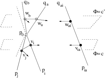
Consider ${\mathfrak{h}}_{ia}$ , the annihilator of the 2-dimensional subspace of ${\mathfrak{g}}^{*}$ generated by $\alpha_{p_{0}p_{i}}$ and $\alpha_{p_{0}q_{a}}$ ; the connected component of $\Gamma_{{\mathfrak{h}}_{ia}}$ that contains $p_{0},p_{i}$ and $q_{a}$ will contain exactly one edge $e_{ia}=(p_{ia},q_{ia})$ that crosses both the $c$ -level and the $c^{\prime}$ -level. To this edge will correspond a neighbor $v_{ia}$ of $v_{i}$ in $\Gamma_{c}$ and a neighbor $w_{ai}$ of $w_{a}$ in $\Gamma_{c^{\prime}}$ .

Let $\mu>0$ and for all $i=1,..,r$ , $a=r+1,..,d$ , define

	$\displaystyle n_{ia}$	$\displaystyle=$	$\displaystyle\mu\alpha_{p_{0}q_{a}}(\xi)>0$		(2.32)
	$\displaystyle n_{ai}$	$\displaystyle=$	$\displaystyle-\mu\alpha_{p_{0}p_{i}}(\xi)>0.$		(2.33)

Denote

\tau_{i}=-\frac{\alpha_{p_{0}p_{i}}}{\mu\alpha_{p_{0}p_{i}}(\xi)}=\frac{\alpha_{p_{0}p_{i}}}{n_{ai}}\quad\mbox{ and }\quad\tau_{a}=\frac{\alpha_{p_{0}q_{a}}}{\mu\alpha_{p_{0}q_{a}}(\xi)}=\frac{\alpha_{p_{0}q_{a}}}{n_{ia}}\;.

Then we have

$\displaystyle\alpha_{v_{i}v_{j}}^{c}$	$\displaystyle=$	$\displaystyle\alpha_{p_{0}p_{j}}-\frac{\alpha_{p_{0}p_{j}}(\xi)}{\alpha_{p_{0}p_{i}}(\xi)}\alpha_{p_{0}p_{i}}=n_{aj}(\tau_{j}-\tau_{i})$
$\displaystyle\alpha_{w_{a}w_{b}}^{c^{\prime}}$	$\displaystyle=$	$\displaystyle\alpha_{p_{0}q_{b}}-\frac{\alpha_{p_{0}q_{b}}(\xi)}{\alpha_{p_{0}q_{a}}(\xi)}\alpha_{p_{0}q_{a}}=n_{ib}(\tau_{b}-\tau_{a})$
$\displaystyle\alpha_{v_{i}v_{ia}}^{c}$	$\displaystyle=$	$\displaystyle\alpha_{p_{0}q_{a}}-\frac{\alpha_{p_{0}q_{a}}(\xi)}{\alpha_{p_{0}p_{i}}(\xi)}\alpha_{p_{0}p_{i}}=n_{ia}(\tau_{a}+\tau_{i})$
$\displaystyle\alpha_{w_{a}w_{ai}}^{c^{\prime}}$	$\displaystyle=$	$\displaystyle\alpha_{p_{0}p_{i}}-\frac{\alpha_{p_{0}p_{i}}(\xi)}{\alpha_{p_{0}q_{a}}(\xi)}\alpha_{p_{0}q_{a}}=n_{ai}(\tau_{i}+\tau_{a}).$

Let $\Gamma_{c}^{0}$ be the sub-skeleton of $\Gamma_{c}$ with vertices $\{v_{1},...,v_{r}\}$ . Along the edge $v_{i}v_{j}$ , the connection transports the edge $v_{i}v_{ia}$ to $v_{j}v_{ja}$ . Noting that $n_{ia}=n_{ja}$ and that

\alpha_{v_{j}v_{ja}}^{c}-\alpha_{v_{i}v_{ia}}^{c}=\frac{n_{ia}}{n_{ja}}\alpha_{v_{i}v_{j}}^{c},

i.e. that $\Gamma_{c}$ satisfies (2.22) on edges of $\Gamma_{c}$ normal to $\Gamma_{c}^{0}$ , we can define the blow-up $\Gamma_{c}^{\#}$ of $\Gamma_{c}$ along $\Gamma_{c}^{0}$ , by means of the positive numbers $n_{ia}$ , $i=1,..,r$ and $a=r+1,..,d$ .

The singular locus, $\Gamma_{0}^{\#}$ , is, as a graph, a product of two complete graphs, $\Gamma_{r}\times\Gamma_{s}$ ; each vertex $z_{ia}$ corresponds to a pair $(v_{i},w_{a})$ and the blow-down map $\beta:\Gamma_{0}^{\#}\to\Gamma_{0}^{c}$ sends $z_{ia}$ to $v_{i}$ .

There are edges connecting $z_{ia}$ with $v_{ia}$ , $z_{ia}$ with $z_{ib}$ and $z_{ia}$ with $z_{ja}$ , for all distinct $i,j=1,..,r$ and $a,b=r+1,..,d$ . The values of the axial function $\alpha^{\#}$ on these edges are

$\displaystyle\alpha_{z_{ia}v_{ia}}^{\#}$	$\displaystyle=$	$\displaystyle\frac{1}{n_{ia}}\alpha_{v_{i}v_{ia}}^{c}=\tau_{a}+\tau_{i}=-\frac{\mu}{n_{ia}n_{ai}}\iota_{\xi}(\alpha_{p_{0}p_{i}}\wedge\alpha_{p_{0}q_{a}})$
$\displaystyle\alpha_{z_{ia}z_{ib}}^{\#}$	$\displaystyle=$	$\displaystyle\alpha_{v_{i}v_{ib}}^{c}-\frac{n_{ib}}{n_{ia}}\alpha_{v_{i}v_{ia}}^{c}=n_{ib}(\tau_{b}-\tau_{a})=$
	$\displaystyle=$	$\displaystyle\frac{\mu}{n_{ai}}\iota_{\xi}(\alpha_{p_{0}q_{a}}\wedge\alpha_{p_{0}q_{b}})$
$\displaystyle\alpha_{z_{ia}z_{ja}}^{\#}$	$\displaystyle=$	$\displaystyle\alpha_{v_{i}v_{j}}^{c}=n_{aj}(\tau_{j}-\tau_{i})=-\frac{\mu}{n_{ai}}\iota_{\xi}(\alpha_{p_{0}p_{i}}\wedge\alpha_{p_{0}p_{j}})$

While $\alpha_{z_{ia}v_{ia}}^{\#}$ and $\alpha_{z_{ia}z_{ib}}^{\#}$ are not collinear (since $\tau_{a},\tau_{b}$ and $\tau_{i}$ are independent), and neither are $\alpha_{z_{ia}v_{ia}}^{\#}$ and $\alpha_{z_{ia}z_{ja}}^{\#}$ , it may happen that $\alpha_{z_{ia}z_{ib}}^{\#}$ and $\alpha_{z_{ia}z_{ja}}^{\#}$ are collinear. We can, however, circumvent this problem by means of the following lemma (which we will leave as an easy exercise).

Lemma 2.2.

Let $\omega_{1},\omega_{2},\omega_{3},\omega_{4}\in{\mathfrak{g}}^{*}$ be 3-independent and suppose that for some $\xi\in{\mathfrak{g}}$ , $\iota_{\xi}(\omega_{1}\wedge\omega_{2})$ and $\iota_{\xi}(\omega_{3}\wedge\omega_{4})$ are collinear. Then the 2-planes generated by $\{\omega_{1},\omega_{2}\}$ and $\{\omega_{3},\omega_{4}\}$ intersect in a line. Moreover, if $\{\omega_{0}\}$ is a basis for this line then $\omega_{0}(\xi)=0$ .

Therefore $\alpha_{z_{ia}z_{ib}}^{\#}$ and $\alpha_{z_{ia}z_{ja}}^{\#}$ are collinear precisely when $\xi$ belongs to a pre-determined hyperplane; so we can insure 2-independence for $\Gamma_{c}^{\#}$ , by avoiding a finite number of such hyperplanes.

Definition 2.3.1.

An element $\xi\in{\mathfrak{g}}$ is called generic for the one-skeleton, $(\Gamma,\alpha)$ , if for every vertex, $p$ , and every quadruple of distinct edges $e_{1},e_{2},e_{3}$ and $e_{4}$ in $E_{p}$ , the vectors $\iota_{\xi}(\alpha_{e_{1}}\wedge\alpha_{e_{2}})$ and $\iota_{\xi}(\alpha_{e_{3}}\wedge\alpha_{e_{4}})$ are linearly independent.

If $\Gamma$ has valence 3 then every element is generic. In general, for every element, $\xi$ , of ${\mathcal{P}}$ and every neighborhood of $\xi$ in ${\mathcal{P}}$ , there exists a generic element, $\xi^{\prime}$ , in that neighborhood, such that the orientations $o_{\xi}$ and $o_{\xi^{\prime}}$ are the same, and the reduced skeleta corresponding to $\xi$ and $\xi^{\prime}$ have isomorphic underlying graphs.

We now return to the proof of Theorem 2.3.2. For a generic $\xi\in{\mathfrak{g}}$ , the blow-up $\Gamma_{c}^{\#}$ can still be defined. Note that

\frac{1}{n_{ia}}\alpha_{v_{i}v_{ia}}^{c}=\frac{1}{n_{ai}}\alpha_{w_{a}w_{ai}}^{c^{\prime}}\quad\mbox{ and that }\quad\alpha_{v_{i}v_{ib}}^{c}-\frac{n_{ib}}{n_{ia}}\alpha_{v_{i}v_{ia}}^{c}=\alpha_{w_{a}w_{b}}^{c^{\prime}}.

These relations imply that $\Gamma_{c}^{\#}$ is the same as the blow-up, $\Gamma_{c^{\prime}}^{\#}$ , of $\Gamma_{c^{\prime}}$ along $\Gamma_{c^{\prime}}^{0}$ using the $n_{ai}$ ’s. Therefore for generic $\xi$ , the passage from $\Gamma_{c}$ to $\Gamma_{c^{\prime}}$ is equivalent to a blow-up from $\Gamma_{c}$ to $\Gamma^{\#}=\Gamma_{c}^{\#}$ followed by a blow-down from $\Gamma^{\#}=\Gamma_{c^{\prime}}^{\#}$ to $\Gamma_{c^{\prime}}$ . ∎

2.3.3. The changes in cohomology

We will now describe how the cohomology changes as one passes from $\Gamma_{c}$ to $\Gamma_{c^{\prime}}$ . For this we will use a variant of Theorem 2.2.1. This theorem itself can’t be applied directly since the reduced one-skeleta might not be 3-independent. However, the proof of Lemma 2.1 is valid up to assertion (2.28) without this assumption and beyond this point it suffices to assume that $\xi$ is generic. Combining Theorems 2.2.1 and 2.1.1 we conclude

$\displaystyle\dim H^{2m}(\Gamma^{\#})$	$\displaystyle=$	$\displaystyle\dim H^{2m}(\Gamma_{c})+\sum_{k=1}^{s-1}\dim H^{2(m-k)}(\Gamma_{r})=$
	$\displaystyle=$	$\displaystyle\dim H^{2m}(\Gamma_{c})+\sum_{k=1}^{s-1}\sum_{l=0}^{r-1}\lambda_{m-k-l}=$
	$\displaystyle=$	$\displaystyle\dim H^{2m}(\Gamma_{c})+\sum_{k=1}^{s-1}\sum_{l=1}^{r-1}\lambda_{m-k-l}+\sum_{k=1}^{s-1}\lambda_{m-k}.$

Therefore

\dim H^{2m}(\Gamma^{\#})=\dim H^{2m}(\Gamma_{c})+\sum_{k=1}^{s-1}\sum_{l=1}^{r-1}\lambda_{m-k-l}+\sum_{k=1}^{s-1}\lambda_{m-k}

and

\dim H^{2m}(\Gamma^{\#})=\dim H^{2m}(\Gamma_{c^{\prime}})+\sum_{l=1}^{r-1}\sum_{k=1}^{s-1}\lambda_{m-k-l}+\sum_{l=1}^{r-1}\lambda_{m-l},

which imply that

\dim H^{2m}(\Gamma_{c^{\prime}})=\dim H^{2m}(\Gamma_{c})+\sum_{k=1}^{s-1}\lambda_{m-k}-\sum_{k=1}^{r-1}\lambda_{m-k}.

(2.34)

(N.B. All $\lambda_{j}$ ’s in the displays above are $\lambda_{j,n-1}$ ’s, since the dimension of ${\mathfrak{g}}_{\xi}^{*}$ is $n-1$ .) Since

\lambda_{a,n}=\sum_{j=0}^{a}\lambda_{j,n-1},

(2.35)

the equality (2.34) can be written as

\dim H^{2m}(\Gamma_{c^{\prime}})=\dim H^{2m}(\Gamma_{c})+\lambda_{m-r,n}-\lambda_{m-s,n}.

(2.36)

2.4. The additive structure of $H(\Gamma,\alpha)$

2.4.1. Symplectic cutting

In this section we will use the results above to draw some conclusions about $H(\Gamma,\alpha)$ itself. This we will do by mimicking, in our graph theoretic setting, the symplectic cutting operation of E. Lerman ([Le]).

Let $L$ be the “edge” graph, with two vertices labeled 0 and 1 and one edge connecting them. Consider $L^{+}=(L,\alpha^{+})$ , with the axial function given by $\alpha_{01}^{+}={\bf 1},\alpha_{10}^{+}=-{\bf 1}$ and $L^{-}=(L,\alpha^{-})$ , with the axial function $\alpha_{01}^{-}=-{\bf 1},\alpha_{10}^{-}={\bf 1}$ . Here $\alpha^{\pm}:E_{L}\to{\mathbb{R}}^{*}\simeq{\mathbb{R}}$ . For ${\mathbb{R}}$ we have the basis $\{1\}$ and for its dual ${\mathbb{R}}^{*}$ the basis $\{{\bf 1}\}$ . For both these axial functions, $1\in{\mathbb{R}}$ is polarizing. Finally, let $\phi_{0}^{\pm}:V_{L}\to{\mathbb{R}}$ be given by $\phi_{0}^{\pm}(0)=0,\phi_{0}^{\pm}(1)=\pm 1$ . Then $\phi_{0}^{\pm}$ is $o_{1}$ -compatible for $\alpha^{\pm}$ .

Let $(\Gamma,\alpha)$ be a one-skeleton which is 3-independent and non-cyclic in the sense of Definition 2.1.3. Let $\phi:V_{\Gamma}\to{\mathbb{R}}$ be $\xi$ -compatible for some $\xi\in{\mathcal{P}}$ and choose $a>\phi_{max}-\phi_{min}>0$ . For $c\in(\phi_{min},\phi_{max})$ let $(\Gamma_{c},\alpha^{c})$ be the reduced one-skeleton of $\Gamma$ at $c$ .

Consider the product one-skeleton $(\Gamma\times L^{+},\alpha\times\alpha^{+})$ , with

\alpha\times\alpha^{+}:E_{\Gamma\times L}\to{\mathfrak{g}}^{*}\oplus{\mathbb{R}}^{*}\simeq({\mathfrak{g}}\oplus{\mathbb{R}})^{*}.

This one-skeleton is also 3-independent and non-cyclic, and the function

\Phi^{+}(p,t)=\phi(p)+a\phi_{0}^{+}(t)=\phi(p)+at

is $(\xi,1)$ -compatible.

Define $\Gamma_{\phi\leq c}$ to be the reduced one-skeleton of $(\Gamma\times L^{+},\alpha\times\alpha^{+})$ at $\Phi^{+}=c$ . The vertices of $\Gamma_{\phi\leq c}$ correspond to two types of edges of $\Gamma\times L^{+}$ :

(1)

$((p_{i},0),(p_{j},0))$ , with $\phi(p_{i})<c<\phi(p_{j})$
(2)

$((p_{i},0),(p_{i},1))$ with $\phi(p_{i})<c$

Let $v_{ij}$ be the vertex of $\Gamma_{\phi\leq c}$ corresponding to an edge $((p_{i},0),(p_{j},0))$ and $w_{i}$ the vertex corresponding to an edge $((p_{i},0),(p_{i},1))$ .

The neighbors of $w_{i}$ are of two types:

(1)

$w_{k}$ , if $(p_{i},p_{k})$ is an edge of $\Gamma$ and $\phi(p_{k})<c$ ;
(2)

$v_{ij}$ , if $(p_{i},p_{j})$ is an edge of $\Gamma$ and $\phi(p_{j})>c$ .

As for neighbors of $v_{ij}$ , apart from $w_{i}$ , they are precisely the neighbors of $v_{ij}$ in the reduced one-skeleton $\Gamma_{c}$ . This $\Gamma_{c}$ sits inside $\Gamma_{\phi\leq c}$ as the subgraph with vertices $v_{ij}$ .

Using (2.30) we deduce that the axial function of $\Gamma_{\phi\leq c}$ , which we will denote by $\beta^{+}$ , is given by:

$\displaystyle\beta_{w_{i}w_{k}}^{+}$	$\displaystyle=$	$\displaystyle\alpha_{p_{i}p_{k}}-\alpha_{p_{i}p_{k}}(\xi)\cdot{\bf 1}$
$\displaystyle\beta_{v_{ij}w_{i}}^{+}$	$\displaystyle=$	$\displaystyle-\frac{1}{\alpha_{p_{j}p_{i}}(\xi)}\alpha_{p_{j}p_{i}}+{\bf 1}$
$\displaystyle\beta_{v_{ij}v_{hr}}^{+}$	$\displaystyle=$	$\displaystyle\alpha_{p_{j}p_{a}}-\frac{\alpha_{p_{j}p_{a}}(\xi)}{\alpha_{p_{j}p_{i}}(\xi)}\alpha_{p_{j}p_{i}}=\alpha_{v_{ij}v_{hr}}^{c}$

The axial function $\beta^{+}$ takes values in $({\mathfrak{g}}\oplus{\mathbb{R}})_{(\xi,1)}^{*}\subset{\mathfrak{g}}^{*}\oplus{\mathbb{R}}^{*}$ . However, there is a natural isomorphism ${\mathfrak{g}}^{*}\rightarrow({\mathfrak{g}}\oplus{\mathbb{R}})_{(\xi,1)}^{*}$ , given by

\sigma\longrightarrow(\sigma,-\sigma(\xi)\cdot{\bf 1}),

(2.37)

so we can regard $\beta^{+}$ as taking values in ${\mathfrak{g}}^{*}$ , and, as such, it is given by:

$\displaystyle\beta_{w_{i}w_{k}}^{+}$	$\displaystyle=$	$\displaystyle\alpha_{p_{i}p_{k}}$
$\displaystyle\beta_{v_{ij}w_{i}}^{+}$	$\displaystyle=$	$\displaystyle-\frac{1}{\alpha_{p_{j}p_{i}}(\xi)}\alpha_{p_{j}p_{i}}$
$\displaystyle\beta_{v_{ij}v_{hr}}^{+}$	$\displaystyle=$	$\displaystyle\alpha_{v_{ij}v_{hr}}^{c}$

Similarly one can define $\Gamma_{\phi\geq c}$ as the reduced one-skeleton of $(\Gamma\times L^{-},\alpha\times\alpha^{-})$ at $\Phi^{-}=c$ , where

\Phi^{-}(p,t)=\phi(p)+a\phi_{0}^{-}(t)=\phi(p)-at

is $(\xi,1)$ -compatible. Note that if $\xi$ is generic then $(\xi,1)$ is generic as well.

2.4.2. The dimension of $H(\Gamma,\alpha)$

We will now apply (2.34) several times to suitable chosen one-skeleta to get the following result, which, in some sense, implies the main results of this article:

Theorem 2.4.1.

Let $(\Gamma,\alpha)$ be a $d$ -valent one-skeleton which is 3-independent and non-cyclic. Then

\dim H^{2m}(\Gamma,\alpha)=\sum_{k=0}^{d}b_{2k}(\Gamma)\lambda_{m-k,n}\;,

(2.38)

the $\lambda^{\prime}$ s being defined by (2.9).

Proof.

Let $\xi\in{\mathfrak{g}}$ be a generic element of ${\mathcal{P}}$ , let $\phi:V_{\Gamma}\to{\mathbb{R}}$ be $\xi$ -compatible and let $\Gamma_{\phi\leq c}$ be the one-skeleton defined in the previous section.

If there is only one vertex $(p,t)$ with $\Phi^{+}(p,t)<c_{0}$ , this one-skeleton is $\Gamma_{d+1}$ , the complete one-skeleton with $d+1$ vertices and if

\phi_{max}<c_{1}<a+\phi_{min}

this one-skeleton is just $(\Gamma,\alpha)$ . Therefore, by studying the change in the cohomology of $\Gamma_{\phi\leq c}$ as $c$ varies, we can determine the additive structure of $H(\Gamma,\alpha)$ from the additive structure of $H(\Gamma_{d+1})$ .

Let $c_{0}<a<b<c_{1}$ such that there is exactly one vertex $p\in V_{\Gamma}$ with $a<\Phi^{+}(p,t)<b$ . If the index of $p$ in $\Gamma$ is $\sigma(p)=r$ then the index of $(p,0)$ in $\Gamma\times L^{+}$ is also $r$ . Note that since the zeroth Betti number of $\Gamma$ is 1, $r$ can’t be 0. Also, in this case, $1\leq s=d+1-r<d+1$ . Thus we can apply (2.34) to obtain

\dim H^{2m}(\Gamma_{\phi\leq b})=\dim H^{2m}(\Gamma_{\phi\leq a})+\sum_{k=1}^{d-r}\lambda_{m-k}-\sum_{k=1}^{r-1}\lambda_{m-k}.

Adding together these changes we get

	$\displaystyle\dim H^{2m}(\Gamma,\alpha)$	$\displaystyle=$	$\displaystyle\dim H^{2m}(\Gamma_{d+1})+\sum_{\sigma(p)>0}\left(\sum_{k=1}^{d-\sigma(p)}\lambda_{m-k}-\sum_{k=1}^{\sigma(p)-1}\lambda_{m-k}\right)=$
		$\displaystyle=$	$\displaystyle\lambda_{m}+\sum_{\sigma(p)\geq 0}\left(\sum_{k=1}^{d-\sigma(p)}\lambda_{m-k}-\sum_{k=1}^{\sigma(p)-1}\lambda_{m-k}\right)$

The minimum value for $k$ is 1 and the maximum is $d$ ; $\lambda_{m-k}$ appears in the first sum when $\sigma(p)\leq d-k$ and in the second one when $\sigma(p)\geq k+1$ . Therefore

\dim H^{2m}(\Gamma,\alpha)=\lambda_{m}+\sum_{k=1}^{d}\left(\sum_{l=0}^{d-k}b_{2l}(\Gamma)-\sum_{l=k+1}^{d}b_{2l}(\Gamma)\right)\lambda_{m-k}.

Because of the relations $b_{2d-2l}(\Gamma)=b_{2l}(\Gamma)$ (see (1.8)) the expression in bracket reduces to $b_{2k}(\Gamma)$ and therefore

\dim H^{2m}(\Gamma,\alpha)=\sum_{k=0}^{d}b_{2k}(\Gamma)\lambda_{m-k,n}\;.

∎

2.4.3. Generators for $H(\Gamma,\alpha)$

We can sharpen the result above by constructing a set of generators for $H(\Gamma,\alpha)$ with nice support conditions. Let $\phi:V_{\Gamma}\to{\mathbb{R}}$ be $\xi$ -compatible for $\xi\in{\mathcal{P}}$ . For $p\in V_{\Gamma}$ , let $F_{p}$ be the flow-out of $p$ , that is the set of vertices of the oriented graph $(\Gamma,o_{\xi})$ that can be reached by a positively oriented path starting from $p$ .

Theorem 2.4.2.

If $p\in V_{\Gamma}$ is a vertex of index $r$ , then there exists an element $\tau_{p}\in H^{2r}(\Gamma,\alpha)$ , with the following properties:

(1)

$\tau_{p}$ is supported on $F_{p}$
(2)

$\tau_{p}(p)=\prod\alpha_{e}$ , the product over edges $e\in E_{p}$ with $\alpha_{e}(\xi)<0$ .

Proof.

We first recall a construction used in [GZ, sec. 2.9]. For every regular value $c\in{\mathbb{R}}$ , let $H_{c}(\Gamma,\alpha)$ be the subring of those maps $f\in H(\Gamma,\alpha)$ that are supported on the set $\phi\geq c$ . Now consider regular values $c,c^{\prime}$ such that there is exactly one vertex, $p$ , satisfying $c<\phi(p)<c^{\prime}$ . Let $r=\sigma(p)$ be the index of $p$ and let $\alpha_{1},..,\alpha_{r}$ be the values of the axial function on the edges pointing down from $p$ . Consider the restriction map

H_{c}^{2m}(\Gamma,\alpha)\to{\mathbb{S}}^{m}({\mathfrak{g}}^{*}),\quad f\to f(p).

The image of this map is contained in $\alpha_{1}\cdots\alpha_{r}{\mathbb{S}}^{m-r}({\mathfrak{g}}^{*})$ , and the kernel is $H_{c^{\prime}}^{2m}(\Gamma,\alpha)$ , so we have an exact sequence

0\to H_{c^{\prime}}^{2m}(\Gamma,\alpha)\to H_{c}^{2m}(\Gamma,\alpha)\to\alpha_{1}\cdots\alpha_{r}{\mathbb{S}}^{m-r}({\mathfrak{g}}^{*}).

(2.39)

Therefore

\dim H_{c}^{2m}(\Gamma,\alpha)-\dim H_{c^{\prime}}^{2m}(\Gamma,\alpha)\leq\lambda_{m-r}.

(2.40)

So when we go from $c<\phi_{min}$ to $c^{\prime}>\phi_{max}$ and add together the inequalities (2.40), we get the inequality

\dim H^{2m}(\Gamma,\alpha)\leq\sum_{r=0}^{d}b_{2r}(\Gamma)\lambda_{m-r}.

(2.41)

But we proved that (2.41) is actually an equality, so all the inequalities (2.40) are equalities, which means that the right arrow in (2.39) is surjective. In particular, when $m=r(=\sigma(p))$ , there exists an element $\tau_{p}^{\prime}\in H_{c}^{2\sigma(p)}(\Gamma,\alpha)$ with

\tau_{p}^{\prime}(p)=\alpha_{1}\cdots\alpha_{r}=\prod_{e\in E_{p},\alpha_{e}(\xi)<0}\alpha_{e},

verifying the second condition. However, to get $\tau_{p}^{\prime}$ to be supported on $F_{p}$ we will need to modify it, and this we will do inductively, as follows:

If $p$ is the vertex where $\phi$ takes its maximum, $F_{p}=\{p\}$ and the first condition is automatically verified. Assume now that we have constructed an element $\tau_{q}$ satisfying both conditions for all vertices, $q$ , above $p$ . We will show that a $\tau_{p}$ exists for $p$ as well. Suppose such an element doesn’t exist and let $p_{1}$ be the highest possible first vertex not in $F_{p}$ where $\tau_{p}^{\prime}$ is non zero, for all choices of $\tau_{p}^{\prime}$ . At all the neighbors of $p_{1}$ below $p_{1}$ , the value of $\tau_{p}^{\prime}$ is zero and therefore $\tau_{p}^{\prime}(p_{1})$ can be written as

\tau_{p}^{\prime}(p_{1})=g\prod_{e\in E_{p_{1}},\alpha_{e}(\xi)<0}\alpha_{e},

for some $g$ . If $\sigma(p_{1})>\sigma(p)=\deg{\tau_{p}^{\prime}}$ then this is possible if and only if $\tau_{p}^{\prime}(p_{1})=0$ , which contradicts the choice of $p_{1}$ . So we must have $\sigma(p_{1})\leq\sigma(p)$ . From the induction hypotheses we know that there exists a $\tau_{p_{1}}$ with the required properties. If we replace $\tau_{p}^{\prime}$ with $\tau_{p}^{\prime\prime}=\tau_{p}^{\prime}-g\tau_{p_{1}}$ then this new element will still satisfy the second condition, will be zero at all vertices not in $F_{p}$ that are below $p_{1}$ but will also be 0 at $p_{1}$ , which contradicts the “maximality” of $\tau_{p}^{\prime}$ .

Therefore an element $\tau_{p}$ must exists for $p$ as well. ∎

The method of proof above also gives us the following uniqueness result.

Theorem 2.4.3.

Suppose that for every point $q\in F_{p}$ , different from $p$ , the index of $q$ is strictly greater than the index of $p$ . Then the class, $\tau_{p}$ , is unique.

We will show that these classes generate $H(\Gamma,\alpha)$ as a module over ${\mathbb{S}}({\mathfrak{g}}^{*})$ .

Theorem 2.4.4.

If $\{\tau_{p}\}_{p\in V_{\Gamma}}$ satisfy the hypotheses of Theorem 2.4.2 then

H^{2m}(\Gamma,\alpha)=\bigoplus_{\sigma(p)\leq m}{\mathbb{S}}^{m-\sigma(p)}({\mathfrak{g}}^{*})\tau_{p}.

In particular, $H(\Gamma,\alpha)$ is a free ${\mathbb{S}}({\mathfrak{g}}^{*})$ -module with the $\tau_{p}$ ’s as generators.

Proof.

We will show that every element $f\in H^{2m}(\Gamma,\alpha)$ can be written uniquely as

f=\sum_{\sigma(p)\leq m}h_{p}\tau_{p},

(2.42)

where $h_{p}\in{\mathbb{S}}^{m-\sigma(p)}({\mathfrak{g}}^{*})$ .

Let $p_{0},p_{1},..,p_{N}$ be the vertices of $\Gamma$ , ordered so that

\phi(p_{0})<\phi(p_{1})<...<\phi(p_{N}).

Then $\tau_{p_{0}}(p_{0})=1$ and, if we let $h_{p_{0}}=f(p_{0})$ ,

f_{0}=f-h_{p_{0}}\tau_{p_{0}},

vanishes at $p_{0}$ . Now, suppose

f_{k}=f-\sum_{\stackrel{{\scriptstyle\scriptstyle i<k}}{{\sigma(p_{i})\leq m}}}h_{p_{i}}\tau_{p_{i}}\in H^{2m}(\Gamma,\alpha),

is supported on $\{p_{k},..,p_{N}\}$ . Then

f_{k}(p_{k})=h\prod_{\alpha_{p_{k},e}(\xi)<0}\alpha_{p_{k},e}.

If $\sigma(p_{k})>m$ , then $f_{k}(p_{k})=0$ and if $\sigma(p_{k})\leq m$ let

f_{k+1}=f_{k}-h_{p_{k}}\tau_{p_{k}}\in H^{2m}(\Gamma,\alpha).

Then $f_{k+1}$ is supported on $\{p_{k+1},..,p_{N}\}$ . Proceeding inductively we conclude that

f_{N}=f-\sum_{\sigma(p)\leq m}h_{p}\tau_{p}

is zero at all vertices, that is, that (2.42) holds. ∎

2.5. The Kirwan map

2.5.1. The Kirwan map

Let $(\Gamma,\alpha)$ be as in Theorem 2.4.1 a one-skeleton which is 3-independent and non-cyclic and let $\phi:V_{\Gamma}\to{\mathbb{R}}$ be an injective function which is $\xi$ -compatible for some $\xi\in{\mathcal{P}}$ . Assume that the conditions of Theorem 2.4.1 are satisfied.

Let ${\mathcal{F}}^{2k}(\Gamma_{c},\alpha^{c})$ be the set of all maps

f:V_{\Gamma_{c}}\to{\mathbb{S}}^{k}({\mathfrak{g}}^{*}_{\xi})\,.

The sum

{\mathcal{F}}(\Gamma_{c},\alpha^{c})=\bigoplus{\mathcal{F}}^{2k}(\Gamma_{c},\alpha^{c})

is a graded ring under point-wise multiplication and by Theorem 1.8.3 one gets a map

{\mathcal{K}}_{c}:H(\Gamma,\alpha)\to{\mathcal{F}}(\Gamma_{c},\alpha^{c}).

Theorem 2.5.1.

${\mathcal{K}}_{c}$ maps $H(\Gamma,\alpha)$ to $H(\Gamma_{c},\alpha^{c})$ .

Proof.

All we need to show is that the image of the map, ${\mathcal{K}}_{c}$ , is indeed in $H(\Gamma_{c},\alpha^{c})$ , that is that ${\mathcal{K}}_{c}(f)$ satisfies the compatibility conditions (1.16) for the reduced one-skeleton.

Let $\{x,y_{1},...,y_{n-1}\}$ be a basis of ${\mathfrak{g}}^{*}$ such that $x(\xi)=1$ and $\{y_{1},...,y_{n-1}\}$ is a basis of ${\mathfrak{g}}_{\xi}^{*}$ . Let $\alpha=\alpha(\xi)(x-\beta(y))\in{\mathfrak{g}}^{*}$ such that $\alpha(\xi)\neq 0$ . Then the map

\rho_{\alpha}:{\mathbb{S}}({\mathfrak{g}}^{*})\rightarrow{\mathbb{S}}({\mathfrak{g}}_{\xi}^{*})

given by the identification ${\mathfrak{g}}_{\xi}^{*}\simeq{\mathfrak{g}}^{*}/{\mathbb{R}}\alpha$ will send $x$ to $x-\alpha/\alpha(\xi)\in{\mathfrak{g}}_{\xi}^{*}$ and $y_{j}$ to $y_{j}$ . Therefore $\rho_{\alpha}$ will send a polynomial $P(x,y)\in{\mathbb{S}}({\mathfrak{g}}^{*})$ to the polynomial $P(x-\alpha/\alpha(\xi),y)=P(\beta(y),y)\in{\mathbb{S}}({\mathfrak{g}}_{\xi}^{*})$ .

Now let $f\in H(\Gamma,\alpha)$ . With the notations in Figure 5 we will show that ${\mathcal{K}}_{c}(f)$ satisfies (1.16) for the edge $v_{i}v_{ia}$ :

{\mathcal{K}}_{c}(f)(v_{ia})-{\mathcal{K}}_{c}(f)(v_{i})\equiv 0\pmod{\alpha_{v_{i}v_{ia}}^{c}}\quad\mbox{ in }{\mathbb{S}}({\mathfrak{g}}_{\xi}^{*}).

(2.43)

For each $j$ we have

\rho_{\alpha_{t_{j}t_{j+1}}}(f_{t_{j}})=f_{t_{j}}(x-\alpha_{t_{j}t_{j+1}}/\alpha_{t_{j}t_{j+1}}(\xi),y)

and therefore the difference

\rho_{\alpha_{t_{j}t_{j+1}}}(f_{t_{j}})-\rho_{\alpha_{t_{j}t_{j-1}}}(f_{t_{j}})

is the same as

f_{t_{j}}(x-\frac{\alpha_{t_{j}t_{j+1}}}{\alpha_{t_{j}t_{j+1}}(\xi)},y)-f_{t_{j}}(x-\frac{\alpha_{t_{j}t_{j-1}}}{\alpha_{t_{j}t_{j-1}}(\xi)},y),

which is a multiple (in $S({\mathfrak{g}}_{\xi}^{*})$ ) of

(x-\frac{\alpha_{t_{j}t_{j+1}}}{\alpha_{t_{j}t_{j+1}}(\xi)})-(x-\frac{\alpha_{t_{j}t_{j-1}}}{\alpha_{t_{j}t_{j-1}}(\xi)})

and, thus, of $\alpha_{v_{i}v_{ia}}^{c}$ . Hence (2.43) follows from the fact that

{\mathcal{K}}_{c}(f)(v_{ia})-{\mathcal{K}}_{c}(f)(v_{i})=\sum_{j=1}^{k}\left(\rho_{\alpha_{t_{j}t_{j+1}}}(f_{t_{j}})-\rho_{\alpha_{t_{j}t_{j-1}}}(f_{t_{j}})\right).

∎

2.5.2. The kernel of the Kirwan map

The following theorem, which describes the kernel of the map above, is the combinatorial analogue of a result of Tolman and Weitsman ([TW1]).

Theorem 2.5.2.

The kernel of the map ${\mathcal{K}}_{c}:H(\Gamma,\alpha)\to H(\Gamma_{c},\alpha^{c})$ consists of those elements $f\in H(\Gamma,\alpha)$ which can be written as a sum $f=h_{+}+h_{-},$ with $h_{\pm}\in H(\Gamma,\alpha)$ such that $h_{+}$ is supported on $\phi>c$ and $h_{-}$ is supported on $\phi<c$ .

Proof.

If $f$ is in the kernel of ${\mathcal{K}}_{c}$ then ${\mathcal{K}}_{c}(f)(v)=0$ for every edge $(p,q)$ with $\phi(p)<c<\phi(q)$ , where $v\in V_{\Gamma}$ is the vertex that corresponds to this edge of $\Gamma$ . Since

0={\mathcal{K}}_{c}(f)(v)=\rho_{\alpha_{pq}}(f_{p})\;\;,

it follows that $f_{p}$ is divisible by $\alpha_{pq}$ . Similarly $f_{q}$ is divisible by $\alpha_{pq}$ .

Consider now the maps, $h_{\pm}$ , of $V_{\Gamma}$ into ${\mathbb{S}}({\mathfrak{g}}^{*}))$ defined by

h_{-}(p)=\left\{\begin{array}[]{ccc}f(p),&\mbox{ if }&\phi(p)<c\\ 0,&\mbox{ if }&\phi(p)>c\end{array}\right.,\qquad h_{+}(q)=\left\{\begin{array}[]{ccc}0,&\mbox{ if }&\phi(q)<c\\ f(q),&\mbox{ if }&\phi(q)>c\end{array}\right.\;.

It is clear that $f=h_{+}+h_{-}$ and that $h_{\pm}\in H(\Gamma,\alpha)$ . ∎

By a slight modification of the proof of Theorem 2.4.4, one can prove the following:

Corollary 2.5.1.

The dimension of $ker\{{\mathcal{K}}_{c}:H^{2m}(\Gamma)\to H^{2m}(\Gamma_{c})\}$ is

\dim{H_{c^{+}}^{2m}(\Gamma)}+\dim{H_{c^{-}}^{2m}(\Gamma)}=\sum_{\phi(q)>c}\lambda_{m-\sigma(q),n}+\sum_{\phi(p)<c}\lambda_{m-d+\sigma(p),n}\;,

where

H_{c^{+}}(\Gamma)=\{h\in H(\Gamma,\alpha);h\mbox{ is supported on }\phi>c\}

and

H_{c^{-}}(\Gamma)=\{h\in H(\Gamma,\alpha);h\mbox{ is supported on }\phi<c\}.

2.5.3. The surjectivity of the Kirwan map

We will finally prove the graph theoretic analogue of Theorem 1.8.1.

Theorem 2.5.3.

For generic $\xi\in{\mathcal{P}}$ , the Kirwan map ${\mathcal{K}}_{c}$ is surjective.

Proof.

We will show that ${\mathcal{K}}_{c}:H(\Gamma,\alpha)\to H(\Gamma_{c},\alpha^{c})$ is surjective by a dimension count, using induction on the number of vertices $p\in V_{\Gamma}$ that lie under the level $\phi=c$ .

To start, assume there is only one such vertex, $p$ . Then $p$ is minimum of $\phi$ and the reduced space $\Gamma_{c}$ is a complete one-skeleton with $d$ vertices, $v_{1},..,v_{d}$ , one for each edge $e_{i}$ issuing from $p$ . Let $f\in H^{2m}(\Gamma_{c},\alpha^{c})$ . Then, by (2.12), there exists $f_{0}\in{\mathbb{S}}({\mathfrak{g}}^{*})\subset H(\Gamma,\alpha)$ such that $\rho_{\alpha_{e_{i}}}(f_{0})=f(v_{i})$ for all $i$ ’s. Hence ${\mathcal{K}}_{c}(f_{0})=f.$

Let’s assume now that the map, ${\mathcal{K}}_{c}$ , is surjective at the level $a$ and choose a regular value $b>a$ such that there is exactly one vertex, $p$ , with $a<\phi(p)<b$ . Let $r=\sigma(p)$ and $s=d-r$ . We have two exact sequences

0\to ker({\mathcal{K}}_{a})\to H^{2m}(\Gamma,\alpha)\stackrel{{\scriptstyle{\mathcal{K}}_{a}}}{{\longrightarrow}}H^{2m}(\Gamma_{a},\alpha^{a})\to 0,

(2.44)

and

0\to ker({\mathcal{K}}_{b})\to H^{2m}(\Gamma,\alpha)\stackrel{{\scriptstyle{\mathcal{K}}_{b}}}{{\longrightarrow}}H^{2m}(\Gamma_{b},\alpha^{b}).

The last arrow in (2.44) is surjective because of our inductive assumption.

By Corollary 2.5.1

\dim{ker({\mathcal{K}}_{b})}-\dim{ker({\mathcal{K}}_{a})}=\lambda_{m-s,n}-\lambda_{m-r,n}

(2.45)

and by (2.45) and (2.36)

\dim{ker({\mathcal{K}}_{b})}+\dim{H^{2m}(\Gamma_{b})}=\dim{ker({\mathcal{K}}_{a})}+\dim{H^{2m}(\Gamma_{a})}\\ +(\lambda_{m-s,n}-\lambda_{m-r,n})+(\lambda_{m-r,n}-\lambda_{m-s,n})=\dim H^{2m}(\Gamma,\alpha).

This proves that

\dim({im({\mathcal{K}}_{b})})=\dim{H^{2m}(\Gamma)}-\dim{ker({\mathcal{K}}_{b})}=\dim{H^{2m}(\Gamma_{b})},

hence that ${\mathcal{K}}_{b}$ is surjective. ∎

3. Applications

3.1. The realization theorem

Recall that an abstract one-skeleton, $(\Gamma,\alpha)$ , is an abstract GKM one-skeleton if $\alpha$ satisfies (2.5) and (2.6) and the constants $c_{i,e}$ in (2.6) are integers. In this section we will prove that all such abstract one-skeleta can be realized as the GKM-skeleta of GKM spaces.

Theorem 3.1.1.

If $(\Gamma,\alpha)$ is an abstract GKM one-skeleton, there exists a complex manifold $M$ and a GKM action of $G$ on $M$ for which $(\Gamma,\alpha)$ is its GKM one-skeleton.

Remarks:

(1)

The manifold $M$ which we will construct below is not compact, and there does not appear to be a canonical compactification of it. For some interesting non-canonical compactifications of it see [GKT].
(2)

The manifold $M$ is also not equivariantly formal, but it does have the property that the canonical map of $H_{G}(M)$ into $H(\Gamma,\alpha)$ is surjective.

Proof.

Our construction of $M$ will involve three steps: first we will construct the ${\mathbb{C}}P^{1}$ ’s corresponding to the edges of $\Gamma$ ; then, for each of these ${\mathbb{C}}P^{1}$ ’s, we will construct a tubular neighborhood of it in $M$ . Then we will construct $M$ itself by gluing these tubular neighborhoods together.

Let $\rho_{\alpha}$ be the one dimensional representation of $G$ with weight $\alpha$ and let $V_{\alpha}\simeq{\mathbb{C}}$ be the vector space on which this representation lives. Let $G$ act on $V_{\alpha}\oplus{\mathbb{C}}$ by acting by $\rho_{\alpha}$ on the first factor and by the trivial representation on the second factor. This action induces an action of $G$ on the projectivization

X_{\alpha}={\mathbb{C}}P^{1}={\mathbb{P}}(V_{\alpha}\oplus{\mathbb{C}}).

(3.1)

The points $q=[1:0]$ and $p=[0:1]$ are the two fixed points of this action and there are equivariant bijective maps

V_{\alpha}\to X_{\alpha}-\{q\},\qquad c\to[c:1],

(3.2)

and

V_{-\alpha}\to X_{\alpha}-\{p\},\qquad c\to[1:c].

(3.3)

(The equivariance of (3.3) follows from the fact that , for $\xi\in{\mathfrak{g}}$ ,

[e^{i\alpha(\xi)}:c]=[1:e^{-i\alpha(\xi)}c].)

We will denote by ${\mathbb{L}}_{\alpha}$ the tautological line bundle over $X_{\alpha}$ . By definition, the fiber of ${\mathbb{L}}_{\alpha}$ over $[c_{1}:c_{2}]$ is the one dimensional subspace of $V_{\alpha}\oplus{\mathbb{C}}$ spanned by $(c_{1},c_{2})$ ; so from the action of $G$ on $V_{\alpha}\oplus{\mathbb{C}}$ one gets an action of $G$ on ${\mathbb{L}}_{\alpha}$ lifting the action of $G$ on $X_{\alpha}$ . The fiber of ${\mathbb{L}}_{\alpha}$ over $q$ is $V_{\alpha}$ , so, in particular, the following is true:

Lemma 3.1.

The weight of the isotropy action of $G$ on $({\mathbb{L}}_{\alpha})_{p}$ is zero and on $({\mathbb{L}}_{\alpha})_{q}$ is $\alpha$ .

The mapping

[c:1]\to(c,1)

(3.4)

defines a holomorphic section of ${\mathbb{L}}_{\alpha}$ over $X_{\alpha}-\{q\}$ , and hence a holomorphic trivialization of the restriction of ${\mathbb{L}}_{\alpha}$ to $X_{\alpha}-\{q\}$ .

The vector space $V_{\alpha}\oplus{\mathbb{C}}\simeq{\mathbb{C}}^{2}$ can be equipped with the $G$ -invariant Hermitian form

|z|^{2}=|z_{1}|^{2}+|z_{2}|^{2}

(3.5)

and since the restriction of this form to each subspace of ${\mathbb{C}}^{2}$ defines a Hermitian form on this subspace, we get from this form a $G$ -invariant Hermitian structure on ${\mathbb{L}}_{\alpha}$ .

Now let $\alpha_{i}$ and $\alpha_{i}^{\prime}$ be weights of $G$ with $\alpha_{i}^{\prime}-\alpha_{i}=m\alpha,$ $m$ being an integer, and let ${\mathbb{L}}_{i}$ be the line bundle

{\mathbb{L}}_{i}={\mathbb{L}}_{\alpha}^{m}\otimes V_{\alpha_{i}}.

(3.6)

From the action of $G$ on ${\mathbb{L}}_{\alpha}$ and on $V_{\alpha_{i}}$ one gets an action of $G$ on this line bundle lifting the action of $G$ on $X_{\alpha}$ . The following is a corollary of Lemma 3.1 and of the existence of the Hermitian structure (3.5) on ${\mathbb{L}}_{\alpha}$ and of the trivialization (3.4) of ${\mathbb{L}}_{\alpha}$ over $X_{\alpha}-\{q\}$ .

Lemma 3.2.

The weight of the isotropy representation of $G$ on $({\mathbb{L}}_{i})_{p}$ is $\alpha_{i}$ and on $({\mathbb{L}}_{i})_{q}$ is $\alpha_{i}^{\prime}$ . In addition, ${\mathbb{L}}_{i}$ has a $G$ -invariant Hermitian structure and a non-vanishing holomorphic section, $s_{i}:X_{\alpha}-\{q\}\to{\mathbb{L}}_{i}$ , which transforms under the action of $G$ according to the weight $\alpha_{i}$ . In particular, the restriction of ${\mathbb{L}}_{i}$ to $X_{\alpha}-\{q\}$ is isomorphic to the trivial bundle over $X_{\alpha}-\{q\}$ with fiber $V_{\alpha_{i}}$ .

Let’s now return to the problem of constructing a manifold $M$ with $(\Gamma,\alpha)$ as its GKM one-skeleton. Let $e$ be an oriented edge of $\Gamma$ and let $p,p^{\prime},e_{i}$ and $e_{i}^{\prime}$ be as in (2.6) with $e_{d}=e$ and $e_{d}^{\prime}=\bar{e}$ . Let $X_{e}=X_{\alpha}$ , with $\alpha=\alpha_{e}$ , and let ${\mathbb{L}}_{i}$ be the line bundle constructed above with $\alpha_{i}=\alpha_{e_{i}}$ and $\alpha_{i}^{\prime}=\alpha_{e_{i}^{\prime}}$ . The $X_{e}$ ’s will be our candidates for the $G$ -invariant ${\mathbb{C}}P^{1}$ ’s in $M$ and the vector bundle

N_{e}=\bigoplus_{i=1}^{d-1}{\mathbb{L}}_{i}

(3.7)

will be our candidate for the normal bundle of $X_{e}$ in $M$ . Thus, a candidate for a tubular neighborhood of $X_{e}$ in $M$ will be a convex neighborhood of the zero section in $N_{e}$ , for example, the disk bundle

{\mathcal{U}}_{e}^{\epsilon}=\{(x,v_{1},..,v_{d-1});x\in X_{e},v_{i}\in({\mathbb{L}}_{i})_{x},|v_{1}|<\epsilon\}.

(3.8)

We will construct $M$ by starting with the disjoint union

\coprod{\mathcal{U}}_{e}^{\epsilon}

(3.9)

over all edges $e$ of $\Gamma$ , and making the following obvious identifications: Let $N_{e,p}$ be the restriction of the bundle $N_{e}$ to $X_{e}-\{q\}$ . By Lemma 3.2 and by (3.2) one gets a $G$ -equivariant bijective map

N_{e,p}\stackrel{{\scriptstyle\gamma_{e}}}{{\longrightarrow}}T_{p}M

(3.10)

where $T_{p}M$ is by definition the sum

\bigoplus_{i=1}^{d}V_{\alpha_{i}}.

(3.11)

If $e$ and $e^{\prime}$ are edges of $\Gamma$ meeting at $p$ we will identify the points $u\in{\mathcal{U}}_{e,p}^{\epsilon}$ and $u^{\prime}\in{\mathcal{U}}_{e^{\prime},p}^{\epsilon}$ in the set (3.9) if

\gamma_{e}(u)=\gamma_{e^{\prime}}(u^{\prime}).

It is easy to check that if we quotient (3.9) by the equivalence relation defined by these identifications (with $\epsilon$ small), we get a manifold $M$ with the properties listed in theorem. ∎

3.2. A deformation problem

We return to the example of section 1.10: the one-skeleton, $\Gamma$ , of an edge-reflecting $d$ -valent convex polytope $\Delta$ embedded into an $n$ -dimensional space ${\mathfrak{g}}^{*}$ by $\Phi:\Delta\to{\mathfrak{g}}^{*}$ , the axial function, $\alpha$ , of $\Gamma$ being given by

\alpha_{pq}=\Phi(q)-\Phi(p).

Fix a vector $\xi\in{\mathcal{P}}$ and let $\phi:V_{\Gamma}\to{\mathbb{R}}$ be given by

\phi(p)=\langle\Phi(p),\xi\rangle\;\quad\mbox{ for all }p\in V_{\Gamma}.

(3.12)

Then $\phi$ is $\xi$ -compatible and the zeroth Betti number of $\Gamma$ is 1; and since every 2-face of $\Delta$ is convex, $\Gamma$ is non-cyclic. Moreover, $\Gamma$ is 3-independent if $\dim{\mathfrak{g}}^{*}\geq 3$ (see the comments at the end of section 1.10).

Assume that there exists a lattice ${\mathbb{Z}}_{G}^{*}$ in ${\mathfrak{g}}^{*}$ such that the edges of $\Delta$ are scalar multiples of rational vectors. If we try to deform $\Delta$ by changing its vertices such that the above property is preserved, we are led to the following definition:

Definition 3.2.1.

A function $f:V_{\Gamma}\to{\mathfrak{g}}^{*}$ is called a rational deformation of $\Phi$ if there exists $\epsilon>0$ such that for every $t\in[0,\epsilon)$ , the map $\Phi_{t}:V_{\Gamma}\to{\mathfrak{g}}^{*}$ given by

\Phi_{t}(p)=\Phi(p)+tf(p)\;,\forall p\in V_{\Gamma}\;,

is an embedding of $V_{\Gamma}$ into ${\mathfrak{g}}^{*}$ and, for every edge $e=(p,q)$ of $\Gamma$ , $\Phi_{t}(q)-\Phi_{t}(p)$ is a positive multiple of $\alpha_{p,e}$ .

Theorem 3.2.1.

For a given embedding $\Phi$ , the space of rational deformations is $H^{2}(\Gamma,\alpha)$ .

Proof.

Let $f$ be a rational deformation. Then

\Phi_{t}(q)-\Phi_{t}(p)=\Phi(q)-\Phi(p)+t(f(q)-f(p));

(3.13)

since $\alpha_{pq}$ divides both $\Phi_{t}(q)-\Phi_{t}(p)$ and $\Phi(q)-\Phi(p)$ , it follows that it divides $f(q)-f(p)$ as well, which means that $f\in H^{2}(\Gamma,\alpha)$ .

Conversely, if $f\in H^{2}(\Gamma,\alpha)$ then (3.13) implies that $\Phi_{t}(q)-\Phi_{t}(p)$ is a multiple of $\alpha_{pq}$ and, since $\Phi(q)-\Phi(p)=\alpha_{pq}$ , for $t$ small enough, it is a positive multiple. We can choose $\epsilon$ small enough for all edges, which proves that $f$ is a rational deformation. ∎

By (2.38)

\dim H^{2}(\Gamma,\alpha)=b_{2}(\Gamma)\lambda_{0}+b_{0}(\Gamma)\lambda_{1}=b_{2}(\Gamma)+n.

(3.14)

Every translation is a rational deformation and the “ $n$ ” in (3.14) is the contribution of these “trivial” deformations to the space of deformations of $\Gamma$ . Hence the non-trivial rational deformations are those corresponding to $b_{2}(\Gamma)$ . By Theorem 2.4.4, these deformations are linear combinations of Thom classes, $\tau_{p}$ , for $p$ of index 1.

Example 3.2.1.

Consider an octahedron embedded in ${\mathbb{R}}^{3}$ ; then $b_{2}(\Gamma)=1$ . All rational deformations are obtained by composing translations with the homothety $p\in V_{\Gamma}\to(1-t)p$ . In Figure 8 the numbers next to vertices indicate the index with respect to the height function. The condition on 2-planes amounts to saying that 04, 22 and 13 intersect in a point.

3.3. Schubert polynomials

For the Grassmannians, the classes $\tau_{p}$ of Theorem 2.4.2 have an alternative description in terms of Schubert polynomials (see [BGG], [LS], [Dem], [KK], [Mac], [BH], [Fu1] et al.). This description involves the Hecke algebra of divided difference operators, an algebra which is intrinsically associated to every compact semisimple Lie group $K$ : Let $G$ be the Cartan subgroup of $K$ and $W=N(G)/G$ the Weyl group. As a group of transformations of ${\mathfrak{g}}$ , $W$ is generated by simple reflections. Moreover, to each reflection $\sigma\in W$ corresponds a unique positive root $\alpha=\alpha_{\sigma}\in{\mathfrak{g}}^{*}$ with $\alpha(\sigma\xi)=-\alpha(\xi)$ for all $\xi\in{\mathfrak{g}}$ . In particular, $\sigma$ leaves fixed the hyperplane $\alpha(\xi)=0$ . The divided difference operator

D_{\sigma}:{\mathbb{S}}({\mathfrak{g}}^{*})\to{\mathbb{S}}({\mathfrak{g}}^{*})

is the operator defined by

D_{\sigma}(f)=\frac{f-\sigma f}{\alpha_{\sigma}}.

(3.15)

(Notice that since $\sigma f(\xi)=f(\sigma(\xi))=f(\xi)$ for $\xi$ on the hyperplane $\alpha(\xi)=0$ , the left hand side of (3.15) is an element of ${\mathbb{S}}({\mathfrak{g}}^{*})$ , that is, a polynomial function on ${\mathfrak{g}}$ .)

The Hecke algebra of divided difference operators ${\mathcal{D}}$ is the algebra generated by the $D_{\sigma}$ ’s and the operators “multiplication by $f$ ” for $f\in{\mathbb{S}}({\mathfrak{g}}^{*})$ . We note that if $g\in{\mathbb{S}}({\mathfrak{g}}^{*})^{W}$ then

D_{\sigma}(gf)=\frac{gf-\sigma(gf)}{\alpha_{\sigma}}=g\frac{f-\sigma f}{\alpha_{\sigma}}=gD_{\sigma}f,

hence, if $D\in{\mathcal{D}}$ , then

D(gf)=gDf,

(3.16)

so the algebra ${\mathcal{D}}$ acts on ${\mathbb{S}}({\mathfrak{g}}^{*})$ as morphisms of $S({\mathfrak{g}}^{*})^{W}$ -modules. More generally, if ${\mathcal{M}}_{0}$ is an $S({\mathfrak{g}}^{*})^{W}$ -module and

{\mathcal{M}}={\mathcal{M}}_{0}\otimes_{S({\mathfrak{g}}^{*})^{W}}{\mathbb{S}}({\mathfrak{g}}^{*})

(3.17)

then one can make ${\mathcal{M}}$ into a ${\mathcal{D}}$ -module by setting

D(m\otimes f)=m\otimes(Df).

(3.18)

(In view of (3.16) this is a well-defined operator on ${\mathcal{M}}$ .)

Now let $M$ be a $K$ -manifold. From the constant map $M\to pt$ one gets a map in cohomology

H_{K}(pt)\to H_{K}(M)

and since

H_{K}(pt)={\mathbb{S}}({\mathfrak{k}}^{*})^{K}={\mathbb{S}}({\mathfrak{g}}^{*})^{W},

this map makes $H_{K}(M)$ into a module over ${\mathbb{S}}({\mathfrak{g}}^{*})^{W}$ . For the following result see, for instance, [GS3, Ch. 6]:

Theorem 3.3.1.

The $G$ -equivariant cohomology ring of $M$ is related to the $K$ -equivariant cohomology ring of $M$ by the following ring-theoretic identity:

H_{G}(M)=H_{K}(M)\otimes_{{\mathbb{S}}({\mathfrak{g}}^{*})^{W}}{\mathbb{S}}({\mathfrak{g}}^{*}).

(3.19)

Therefore, by (3.17) and (3.18) we conclude:

Theorem 3.3.2.

The $G$ -equivariant cohomology ring $H_{G}(M)$ is canonically a module over ${\mathcal{D}}$ .

Suppose now that $M$ is a GKM manifold and is equivariantly formal. Then, by Theorem 1.7.3,

H_{G}(M)\simeq H(\Gamma,\alpha);

so, we can transport this ${\mathcal{D}}$ -module structure to $H(\Gamma,\alpha)$ . In particular, we get an action of the divided difference operator $D_{\sigma}$ on $H(\Gamma,\alpha)$ .

Theorem 3.3.3.

Let $f:V_{\Gamma}\to{\mathbb{S}}({\mathfrak{g}}^{*})$ be a map which satisfies the compatibility conditions (1.16) (in other words, which belongs to $H(\Gamma,\alpha)$ ). Then, for $p\in V_{\Gamma}$ ,

(D_{\sigma}f)(p)=\frac{f(p)-\sigma(f(\sigma^{-1}p))}{\alpha_{\sigma}}.

(3.20)

Remarks:

(1)

Since $W$ is by definition $N(G)/G$ , it acts on the fixed point set $M^{G}$ . Since $M^{G}=V_{\Gamma}$ , the expression $\sigma^{-1}p$ on the left hand side is unambiguously defined.
(2)

Since $W$ acts on ${\mathbb{S}}({\mathfrak{g}}^{*})$ by ring automorphisms, the ring automorphism $\sigma$ , applied to the element $f(\sigma^{-1}p)\in{\mathbb{S}}({\mathfrak{g}}^{*})$ on the left hand side is also unambiguously defined.
(3)

For a proof of Theorem 3.3.3 see [GHZ].

We now return to section 1.11 and the Bruhat structure of the Johnson graph. Let $\phi$ be the Morse function (1.39) and let $p\in V_{\Gamma}$ be a vertex of $\Gamma$ of index $r$ . Let $p_{0}$ be the unique maximum of $\phi$ , that is

p_{0}=p_{S}\quad,\quad S=\{l+1,..,n\}

with $l=n-k$ and let

\Delta=\prod_{e\in E_{p_{0}}}\alpha_{e}=\prod_{i\leq k<j}(\alpha_{i}-\alpha_{j}).

(3.21)

By Theorem 2.4.2, the Thom class $\tau_{p_{0}}$ is the map

\tau_{p_{0}}:V_{\Gamma}\to{\mathbb{S}}({\mathfrak{g}}^{*})

which takes the value $\Delta$ at $p_{0}$ and 0 everywhere else. Now let $\sigma_{i_{1}},...,\sigma_{i_{s}}$ ( $s=kl-r$ ) be the elementary reflections with the properties described in Theorem 1.11.6. By applying the operator

D_{\sigma_{i_{1}}}\circ...\circ D_{\sigma_{i_{s}}}

to $\tau_{p_{0}}$ one gets a cohomology class $\tau_{p}^{\prime}$ , which is of degree $r=kl-s$ and which, by (1.44), (1.45) and (3.20), is supported on $F_{p}$ . Moreover, it is easy to see that

\tau_{p}(p)=\prod\alpha_{e},

the product being over the down-ward pointing edges $e\in E_{p}$ . Thus, by Theorem 2.4.3 and (1.39), $\tau_{p}=\tau_{p}^{\prime}$ .

Remark.

One can regard the $\tau_{p}$ ’s as being a doubly indexed family of polynomials $f_{p,q}=\tau_{p}(q)$ , indexed by pairs $(p,q)$ of vertices of $\Gamma$ with $p\prec q$ . These polynomials, which are called double Schubert polynomials, have been studied extensively by Billey, Haiman, Stanley, Fomin, Kirillov, Jockusch and others. (For a succinct and engrossing account of what is known about these polynomials we recommend, as collateral reading, the beautiful monograph “ Young Tableaux” by William Fulton, which has just been published by Cambridge University Press.)

References

[AB1] M. F. Atiyah and R. Bott, The moment map and equivariant cohomology, Topology 23 (1984), no. 1, 1-28.
[At] M. F. Atiyah, Convexity and commuting Hamiltonians, Bull.London Math.Soc. 14 (1982), no. 1, 1-15.
[BB] A. Bialynicki-Birula, Some theorems on actions of algebraic groups, Ann. of Math. (2) 98 (1973), 480-497.
[BCN] A.E. Brouwer, A.M. Cohen and A. Neumaier, Distance-regular graphs, Results in Mathematics and Related Areas (3), 18, Springer-Verlag, Berlin - New York, 1989.
[BGG] I.N. Bernstein, I.M. Gelfand and S.I. Gelfand, Schubert cells and cohomology of the spaces $G/P$ , Russian Math. Surveys 28:3 (1973), 1-26.
[BH] S. Billey and M. Haiman, Schubert polynomials for the classical group, J. Amer.Math.Soc. 8 (1995), no. 2, 443-482.
[Bi] S. Billey, Kostant polynomials and the cohomology ring for $G/B$ , Duke Math. J. 96 (1999), no. 1, 205-224.
[Bo] A. Borel, Seminar on transformation groups, Ann. of Math. Studies 46, Princeton Univ. Press, Princeton, NJ 1960.
[BP] M. Brion and C. Procesi, Action d’un tore dans une variété projective, Progr.Math. 92, Birkhäuser, Boston, MA 1990.
[BV] N. Berline and M. Vergne, Classes caractéristiques équivariantes. Formule de localisation en cohomologie équivariante, C.R. Acad. Sci.Sér I Math 295 (1982), no. 9, 539-541.
[CW] H. Crapo and W. Whiteley, Spaces of stresses, projections, and parallel drawings for spherical polyhedra, Beitraege zur Algebra und Geometrie / Contributions to Algebra and Geometry 35 (1994), 259-281.
[Del] T. Delzant, Hamiltoniens périodiques et image convexe de l’application moment, Bull.Soc.Math.France 116 (1988), no. 3, 315-339.
[Dem] M. Demazure, Désingularization des variétés de Schubert généralisées, Ann.Sci.École Norm. Sup.(4) 7 (1974), no. 4, 53-88.
[Fu1] W. Fulton, Flags, Schubert polynomials, degeneracy loci, and determinantal formulas, Duke Math. J. 65 (1992), no. 3, 381-420.
[Fu2] W. Fulton, Young Tableaux.With applications to representation theory and geometry, London Math.Soc.Stud. Texts 35, Cambridge Univ. Press, Cambridge 1997.
[GKM] M. Goresky, R. Kottwitz and R. MacPherson, Equivariant cohomology, Koszul duality, and the localization theorem, Invent. Math. 131 (1998),no. 1, 25-83.
[GKT] V. Ginzburg, Y. Karshon and S. Tolman, in preparation.
[GHZ] V. Guillemin, T. Holm and C. Zara, GKM-theory on homogeneous manifolds, in preparation
[Go] L. Godinho, Circle actions on symplectic manifolds, Thesis, SUNY Stony Brook 1999.
[GS1] V. Guillemin and S. Sternberg, Convexity properties of the moment mapping, Invent. Math. 67 (1982), no. 3, 491-513.
[GS2] V. Guillemin and S. Sternberg, Birational equivalence in the symplectic category, Invent. Math. 97 (1989), no. 3, 485-522.
[GS3] V. Guillemin and S. Sternberg, Supersymmetry and equivariant de Rham theory, Springer Verlag, Berlin 1999.
[GZ] V. Guillemin and C. Zara, Equivariant de Rham theory and graphs, Asian J. of Math., 3 (1999), no. 1, 44-76.
[Hu] J. Humphreys, Reflection groups and Coxeter groups, Cambridge Stud. in Adv. Math. 29, Cambridge Univ. Press, Cambridge 1990.
[Ja] N. Jacobson, Cayley numbers and normal simple Lie algebras of type $G$ , Duke Math. J. 5 (1939), 775-783.
[Ki] F. Kirwan, Cohomology of quotients in symplectic and algebraic geometry, Math. Notes 31, Princeton Univ. Press, Princeton, NJ 1984.
[Kl] A.A. Klyashko, Equivariant bundles on toric varieties, Math USSR Izvestiya 35 (1990) no. 2, 337-375
[KK] B. Kostant and S. Kumar, The nil Hecke ring and cohomology of $G/P$ for a Kac-Moody group $G$ , Adv. in Math. 62 (1986), no. 3, 187-237.
[KN] S. Kobayashi and K. Nomizu, Foundations of Differential Geometry, vol. II, Interscience Publishers, New York 1969.
[Le] E. Lerman, Symplectic cuts, Math. Res. Lett. 2 (1995), no. 3, 247-258.
[LS] A. Lascoux and M.P. Schützenberger, Schubert polynomials and the Littlewood-Richardson rule, Lett. Math. Phys. 10 (1985), no. 2-3, 111-124.
[LLY] B.H. Lian, K. Liu and S.T. Yau, Mirror symmetry, a survey, Current Developments in Math. 1998, International Press 1998.
[LT] E. Lerman and S. Tolman, Hamiltonian torus actions on symplectic orbifolds and toric varieties, Trans. AMS 349 (1997), 4201-4230.
[Mac] I.G. Macdonald, Schubert polynomials, Surveys in Combinatorics, London Math.Soc.Lect.Note Ser. 166, 73-99, Cambridge Univ. Press, (1991b), Cambridge 1991.
[McD] D. McDuff, Examples of simply-connected symplectic non-Kählerian manifolds, J. Diff. Geom. 20 (1984), no. 1, 267-277.
[Me] E. Meinrenken, Symplectic surgery and the $Spin^{c}$ -Dirac operator, Adv. in Math. 134 (1998), no. 2, 240-277
[St] R. Stanley, Combinatorics and commutative algebra, Progr. in Math. 41, Birkhäuser, Boston, MA 1983.
[TW1] S. Tolman, J. Weitsman, The cohomology rings of abelian symplectic quotients, math.DG/9807173.
[TW2] S. Tolman, J. Weitsman, On the cohomology rings of Hamiltonian T-spaces, math.DG/9812006