跳到论文正文
W Papers独立论文阅读器 arXiv:math/9902151 论文正文 计算阅读时间 · 0%
引用这篇论文根据当前论文元数据生成,正式投稿前建议核对。


License: Assumed arXiv.org perpetual non-exclusive license
arXiv:math/9902151v5 [math.CT] 27 Feb 2000

Homotopy invariants of higher dimensional categories and concurrency in computer science

Philippe Gaucher Affiliation: Institut de Recherche Mathématique Avancée Affiliation: U.L.P. et C.N.R.S. Affiliation: 7 rue René Descartes Affiliation: 67084 Strasbourg Cedex Affiliation: France Affiliation: email : gaucher@irma.u-strasbg.fr
December 1999
Abstract

The strict globular ω\omega-categories formalize the execution paths of a parallel automaton and the homotopies between them. One associates to such (and any) ω\omega-category 𝒞\mathcal{C} three homology theories. The first one is called the globular homology. It contains the oriented loops of 𝒞\mathcal{C}. The two other ones are called the negative (resp. positive ) corner homology. They contain in a certain manner the branching areas of execution paths or negative corners (resp. the merging areas of execution paths or positive corners) of 𝒞\mathcal{C}. Two natural linear maps called the negative (resp. the positive ) Hurewicz morphism from the globular homology to the negative (resp. positive) corner homology are constructed. We explain the reason why these constructions allow the reinterpretation of some geometric problems coming from computer science.

1 Introduction

The use of geometric notions to describe the behaviour of concurrent machines is certainly not new since progress graphs [Dij68], HDA [Pra91][vG91] and simplicial models of [HS94] [HR94]. The purpose of this article is to provide a new setting for the homotopy of execution paths in concurrent automata, in order to improve the homological approach of [Gou95]. We can point out that some other approaches of this question already exist. With partially ordered topological spaces in [FGR98a]. And with partial posets in [Sok99]. Pratt already noticed that a good structure to deal with execution paths and homotopies between them is the structure of globular ω\omega-category [Pra91]. The aim of this paper is threefold. First the use of the concept of globular ω\omega-category to describe concurrent machines is justified on some well-known examples and in a very informal way. Secondly we associate to every globular ω\omega-category three homology theories and two natural maps between them. We explain why their content is interesting for some geometric problems coming from computer science. Thirdly, as in algebraic topology, a notion of homotopic ω\omega-categories is proposed and we prove that the preceding homology theories are invariant with respect to it (only in a particular case for the corner homologies).

Now here is the organization of the paper. In Section 2, we make precise the notion of paths and homotopies between paths, homotopies between homotopies, etc… The notion of globular ω\omega-category is recalled. The link between the usual formalization of concurrent automata using cubical sets and the new formalization by globular ω\omega-categories is explained. We give in a very informal way the geometric and computer science meaning of the homology theories which will be constructed in this paper. In Section 3, the globular homology of a globular ω\omega-category is defined. Some examples of globular cycles are given and the globular complex is related to a derived functor. Section 4 is devoted to the construction of the negative and positive corner homologies of an ω\omega-category. Afterwards we introduce in Section 5 a technical tool to fill shells in the cubical singular nerve of an ω\omega-category. Next in Section 6, this notion of filling of shell is used to construct two families of connections on the cubical singular nerve of an ω\omega-category. It allows us to prove that the corner homologies are the homologies associated to two new simplicial nerves. Afterwards we construct in Section 7 the two natural maps from the globular homology to the negative and positive corner homologies. In Section 8, a notion of homotopy equivalence of ω\omega-categories is proposed. We will prove the following property : Let ff and gg be two non 11-contracting ω\omega-functors from 𝒞\mathcal{C} to 𝒟\mathcal{D}. If ff and gg are homotopic, then for any natural number nn, Hng​l​(f)=Hng​l​(g)H_{n}^{gl}(f)=H_{n}^{gl}(g) (Theorem 8.6). In a very particular case, it is also possible to relate the homotopy of paths in ω\omega-categories to the corner homology theories Hn−H_{n}^{-} and Hn+H_{n}^{+} (Theorem 8.7). In Section 9, some conjectures and perspectives both in mathematics and computer science are exposed. In Section 10, we prove that the cubical singular nerve of the free ω\omega-category generated by a cubical set KK is nothing else but the free cubical ω\omega-category generated by KK. It allows us to propose a direct construction of the globular homology and of the corner homologies of a cubical set without using any globular ω\omega-category.

2 Presentation of the geometric ideas of this work

2.1 Execution paths and homotopies between them in a very informal way

A sequential machine (i.e. without concurrency) is a set of states, also called 00-transitions, and a set of 11-transitions from a given state to another one. A concurrent machine, like the previous one, consists of a set of states and a set of 11-transitions but has also the capability of carrying out several 11-transitions at the same time.

In Figure 1, if we work in cartesian coordinates in such a way that A=[0,1]×[0,1]A=[0,1]\times[0,1] with α=(0,0)\alpha=(0,0) and δ=(1,1)\delta=(1,1), the set of continuous maps (c1,c2)(c_{1},c_{2}) from [0,1][0,1] to AA such that c1​(0)=c2​(0)=0c_{1}(0)=c_{2}(0)=0, c1​(1)=c2​(1)=1c_{1}(1)=c_{2}(1)=1 and t⩽t′t\leqslant t^{\prime} implies c1​(t)⩽c1​(t′)c_{1}(t)\leqslant c_{1}(t^{\prime}) and c2​(t)⩽c2​(t′)c_{2}(t)\leqslant c_{2}(t^{\prime}) represents all the simultaneous possible executions of uu and vv. Coordinates represent the evolution of uu and vv, that means the local time taken to execute uu or vv. If (c1,c2)​(]0,1[)(c_{1},c_{2})(]0,1[) is entirely included in the interior of AA, it is a “true parallelism”. If (c1,c2)​(]0,1[)(c_{1},c_{2})(]0,1[) is entirely included in the edge of the square, that means that uu and vv are sequentially carried out by the automaton. More generally, the concurrent execution of nn 11-transitions can be represented by a nn-cube. This is already noticed for example in [Pra91] and [Gou95].

Definition 2.1.

A cubical set consists of a family of sets (Kn)n⩾0(K_{n})_{n\geqslant 0}, of a family of face maps Kn\textstyle{K_{n}\ignorespaces\ignorespaces\ignorespaces\ignorespaces}∂iα\scriptstyle{\partial_{i}^{\alpha}}Kn−1\textstyle{K_{n-1}} for α∈{−,+}\alpha\in\{-,+\} and of a family of degeneracy maps Kn−1\textstyle{K_{n-1}\ignorespaces\ignorespaces\ignorespaces\ignorespaces}ϵi\scriptstyle{\epsilon_{i}}Kn\textstyle{K_{n}} with 1⩽i⩽n1\leqslant i\leqslant n which satisfy the following relations

  1. 1.

    ∂iα∂jβ=∂j−1β∂iα\partial_{i}^{\alpha}\partial_{j}^{\beta}=\partial_{j-1}^{\beta}\partial_{i}^{\alpha} for all i<j⩽ni<j\leqslant n and α,β∈{−,+}\alpha,\beta\in\{-,+\}

  2. 2.

    ϵi​ϵj=ϵj+1​ϵi\epsilon_{i}\epsilon_{j}=\epsilon_{j+1}\epsilon_{i} for all i⩽j⩽ni\leqslant j\leqslant n

  3. 3.

    ∂iαϵj=ϵj−1∂iα\partial_{i}^{\alpha}\epsilon_{j}=\epsilon_{j-1}\partial_{i}^{\alpha} for i<j⩽ni<j\leqslant n and α∈{−,+}\alpha\in\{-,+\}

  4. 4.

    ∂iαϵj=ϵj∂i−1α\partial_{i}^{\alpha}\epsilon_{j}=\epsilon_{j}\partial_{i-1}^{\alpha} for i>j⩽ni>j\leqslant n and α∈{−,+}\alpha\in\{-,+\}

  5. 5.

    ∂iαϵi=I​d\partial_{i}^{\alpha}\epsilon_{i}=Id

The corresponding category of cubical sets, with an obvious definition of its morphisms, is isomorphic to the category of presheaves S​e​t​s□o​pSets^{\square^{op}} over a small category □\square. This latter can be described in a nice way as follows [Cra95]. The objects of □\square are the sets n¯={1,…,n}\underline{n}=\{1,...,n\} where nn is a natural number greater or equal than 11 and an arrow ff from n¯\underline{n} to m¯\underline{m} is a function f∗f^{*} from m¯\underline{m} to n¯∪{−,+}\underline{n}\cup\{-,+\} such that f∗​(k)⩽f∗​(k′)∈n¯f^{*}(k)\leqslant f^{*}(k^{\prime})\in\underline{n} implies k⩽k′k\leqslant k^{\prime} and f∗​(k)=f∗​(k′)∈n¯f^{*}(k)=f^{*}(k^{\prime})\in\underline{n} implies k=k′k=k^{\prime}.

Let XX be a topological space. Let [0,1][0,1] denote the interval between 00 and 11. Set Kn=C0​([0,1]n,X)K_{n}=C^{0}([0,1]^{n},X) the set of continuous maps from the nn-box [0,1]n[0,1]^{n} to XX. Set

∂i−(f)​(x1,…,xp)=f⁡(x1,…,[0]i,…,xp)\displaystyle\partial_{i}^{-}(f)(x_{1},\dots,x_{p})=f(x_{1},\dots,[0]_{i},\dots,x_{p})
∂i+(f)​(x1,…,xp)=f⁡(x1,…,[1]i,…,xp)\displaystyle\partial_{i}^{+}(f)(x_{1},\dots,x_{p})=f(x_{1},\dots,[1]_{i},\dots,x_{p})
ϵi​(f)​(x1,…,xp)=f⁡(x1,…,xi^,…,xp)\displaystyle\epsilon_{i}(f)(x_{1},\dots,x_{p})=f(x_{1},\dots,\widehat{x_{i}},\dots,x_{p})

Then we obtain a cubical set KK which is called the cubical singular nerve of the topological space XX.

In Figure 1, we call AA an homotopy between the two 11-paths u​v′uv^{\prime} and v​u′vu^{\prime}. We call 22-path an homotopy between two 11-paths and by induction on n⩾2n\geqslant 2, we call nn-path an homotopy between two (n−1)(n-1)-paths. This notion of homotopy is different from the classical one in the sense that only the 11-paths u​v′uv^{\prime} and v​u′vu^{\prime} are homotopic and because the 11-paths are oriented. For example, still in Figure 1, uu is homotopic neither with u′u^{\prime} nor with vv or v′v^{\prime}.

β\textstyle{{\beta}\ignorespaces\ignorespaces\ignorespaces\ignorespaces}v′\scriptstyle{v^{\prime}}δ\textstyle{{\delta}}α\textstyle{{\alpha}\ignorespaces\ignorespaces\ignorespaces\ignorespaces\ignorespaces\ignorespaces\ignorespaces\ignorespaces}u\scriptstyle{u}v\scriptstyle{v}γ\textstyle{{\gamma}\ignorespaces\ignorespaces\ignorespaces\ignorespaces\ignorespaces\ignorespaces\ignorespaces\ignorespaces}A\scriptstyle{A}u′\scriptstyle{u^{\prime}}
Figure 1: A 22-transition

In Figure 2, there are an initial state α\alpha, a final state β\beta, two 11-transitions uu and vv and two 22-transitions or homotopies AA and BB between uu and vv. Choosing an orientation for AA and BB, for example s1​A=s1​B=us_{1}A=s_{1}B=u and t1​A=t1​B=vt_{1}A=t_{1}B=v (ss for source and tt for target), we see that s0​s1​A=s0​t1​A=αs_{0}s_{1}A=s_{0}t_{1}A=\alpha and t0​s1​A=t0​t1​A=βt_{0}s_{1}A=t_{0}t_{1}A=\beta. These are precisely the globular equations which appear in the axioms of globular ω\omega-categories.

Figure 2: A 33-dimensional hole

The concatenation yields an associative composition law on the set of 11-transitions of an ω\omega-category. It turns out that there is also a natural composition law on the set of 22-transitions. In Figure 3, with the convention of orientation t1​A=s1​Bt_{1}A=s_{1}B, we can compose AA and BB. Denote this composition by A∗1BA*_{1}B. We see that s1​(A∗1B)=s1​As_{1}(A*_{1}B)=s_{1}A, t1​(A∗1B)=t1​Bt_{1}(A*_{1}B)=t_{1}B. The composition of higher dimensional morphisms must be associative because it corresponds to the concatenation of the real execution paths contained in AA and BB.

α\textstyle{{\alpha}\ignorespaces\ignorespaces\ignorespaces\ignorespaces\ignorespaces\ignorespaces\ignorespaces\ignorespaces}A\textstyle{\scriptstyle A}B\textstyle{\scriptstyle B}β\textstyle{{\beta}}
Figure 3: Composition of two 22-morphims

Thus the geometric properties of transitions of concurrent machines can be encoded in a structure of cubical set. And their associated set of execution paths and homotopies between them have a natural structure of globular ω\omega-category. All these ideas already appear in [Pra91]. Pratt uses the term of nn-complex which is in fact nothing else but a small nn-category. We use the notations of [Ste91] and [Str87] for the following definition. The following definition already appears in [BH81a]

Definition 2.2.

An ω\omega-category is a set AA endowed with two families of maps (sn=dn−)n⩾0(s_{n}=d_{n}^{-})_{n\geqslant 0} and (tn=dn+)n⩾0(t_{n}=d_{n}^{+})_{n\geqslant 0} from AA to AA and with a family of partially defined 2-ary operations (∗n)n⩾0(*_{n})_{n\geqslant 0} where for any n⩾0n\geqslant 0, ∗n*_{n} is a map from {(a,b)∈A×A,tn​(a)=sn​(b)}\{(a,b)\in A\times A,t_{n}(a)=s_{n}(b)\} to AA ((a,b)(a,b) being carried over a∗nba*_{n}b) which satisfies the following axioms for all α\alpha and β\beta in {−,+}\{-,+\} :

  1. 1.

    dmβdnαx={dmβ​x​ if m<ndnα​x​ if m⩾nd_{m}^{\beta}d_{n}^{\alpha}x=\left\{\begin{CD}d_{m}^{\beta}x\hbox{ if $m<n$}\\ d_{n}^{\alpha}x\hbox{ if $m\geqslant n$}\end{CD}\right.

  2. 2.

    sn​x∗nx=x∗ntn​x=xs_{n}x*_{n}x=x*_{n}t_{n}x=x

  3. 3.

    if x∗nyx*_{n}y is well-defined, then sn​(x∗ny)=sn​xs_{n}(x*_{n}y)=s_{n}x, tn​(x∗ny)=tn​yt_{n}(x*_{n}y)=t_{n}y and for m≠nm\neq n, dmα​(x∗ny)=dmα​x∗ndmα​yd_{m}^{\alpha}(x*_{n}y)=d_{m}^{\alpha}x*_{n}d_{m}^{\alpha}y

  4. 4.

    as soon as the two members of the following equality exist, then (x∗ny)∗nz=x∗n(y∗nz)(x*_{n}y)*_{n}z=x*_{n}(y*_{n}z)

  5. 5.

    if m≠nm\neq n and if the two members of the equality make sense, then (x∗ny)∗m(z∗nw)=(x∗mz)∗n(y∗mw)(x*_{n}y)*_{m}(z*_{n}w)=(x*_{m}z)*_{n}(y*_{m}w)

  6. 6.

    for any xx in AA, there exists a natural number nn such that sn​x=tn​x=xs_{n}x=t_{n}x=x (the smallest of these numbers is called the dimension of xx and is denoted by d​i​m​(x)dim(x)).

We will sometimes use the notations dn−:=snd^{-}_{n}:=s_{n} and dn+=tnd^{+}_{n}=t_{n}. If xx is a morphism of an ω\omega-category 𝒞\mathcal{C}, we call sn​(x)s_{n}(x) the nn-source of xx and tn​(x)t_{n}(x) the nn-target of xx. The category of all ω\omega-categories (with the obvious morphisms) is denoted by ω​C​a​t\omega Cat. The corresponding morphisms are called ω\omega-functors.

If SS is a set, the free abelian group generated by SS is denoted by ℤ​S\mathbb{Z}S. By definition, an element of ℤ​S\mathbb{Z}S is a formal linear combination of elements of SS.

Definition 2.3.

Let 𝒞\mathcal{C} be an ω\omega-category. Let 𝒞n\mathcal{C}_{n} be the set of nn-dimensional morphisms of 𝒞\mathcal{C}. Two nn-morphisms xx and yy are homotopic if there exists z∈ℤ​𝒞n+1z\in\mathbb{Z}\mathcal{C}_{n+1} such that sn​z−tn​z=x−ys_{n}z-t_{n}z=x-y. This property is denoted by x∼yx\sim y.

If x∼yx\sim y, then the pair (x,y)(x,y) belongs to the reflexive, symmetric and transitive closure of the binary relation generated by all pairs (sn​(u),tn​(u))(s_{n}(u),t_{n}(u)) where uu runs over 𝒞n+1\mathcal{C}_{n+1}.

γ1=u∗0v∗0w∗0x∗0y∗0z\displaystyle\gamma_{1}=u*_{0}v*_{0}w*_{0}x*_{0}y*_{0}z
γ2=u∗0a∗0b∗0x∗0c∗0d\displaystyle\gamma_{2}=u*_{0}a*_{0}b*_{0}x*_{0}c*_{0}d
γ3=u∗0v∗0w∗0x∗0c∗0d\displaystyle\gamma_{3}=u*_{0}v*_{0}w*_{0}x*_{0}c*_{0}d
γ4=e∗0f∗0g∗0h∗0i∗0d\displaystyle\gamma_{4}=e*_{0}f*_{0}g*_{0}h*_{0}i*_{0}d
Figure 4: Example of distributed database

Figure 4 is a very simple example of a distributed database. The hole in the middle corresponds to a mutual exclusion. See [FGR98b] for a complete treatment. The two 11-paths γ1\gamma_{1} and γ2\gamma_{2} are homotopic because there exists a 22-morphism between γ1\gamma_{1} and γ3\gamma_{3} and another one between γ2\gamma_{2} and γ3\gamma_{3}. On the other hand none of the previous three 11-paths is homotopic to γ4\gamma_{4} because of the oriented hole in the middle.

2.2 The free ω\omega-category generated by a cubical set

How may we mathematically associate to every cubical set KK its corresponding set of execution paths and higher dimensional homotopies ? The link between the two formalizations is as follows. We need to describe precisely the free ω\omega-category associated to each nn-cube of KK. In a very informal way, it consists of seeing the faces of a nn-cube as words of length nn in the alphabet {−,0,+}\{-,0,+\}. The term 0n0_{n} means 00 nn times, i.e. the interior of the nn-cube. And we say that the face k1​…​knk_{1}\dots k_{n} is at the source of xx if ki≠0k_{i}\neq 0 implies ki=(−1)ik_{i}=(-1)^{i} and we say that k1​…​knk_{1}\dots k_{n} is at the target of xx if ki≠0k_{i}\neq 0 implies ki=(−1)i+1k_{i}=(-1)^{i+1}. We will make precise the construction of InI^{n} in Section 4.1. Once this is done, it suffices to paste the ω\omega-categories associated to every nn-cube of KK in the same way that they are pasted in KK. More concretely, every cubical set KK is in a canonical way the direct limit of the elementary nn-cubes included in it. This is due to the fact that any functor from a small category to the category S​e​t​sSets of sets is a canonical direct limit of representable functors, the set of those functors being dense in the set of all set-valued functors. More precisely, we have K=∫n¯∈□Kn.□⁡(−,n¯)K=\int^{\underline{n}\in\square}K_{n}.\square(-,\underline{n}) where the integral sign is the coend construction [ML71] and Kn.□⁡(−,n¯)K_{n}.\square(-,\underline{n}) means the sum of “cardinal of KnK_{n}” copies of □⁡(−,n¯)\square(-,\underline{n}). So F⁡(K)=∫n¯∈□Kn.InF(K)=\int^{\underline{n}\in\square}K_{n}.I^{n} is a ω\omega-category containing as 11-morphisms all arrows of KK and all possible compositions of these arrows, as 22-morphisms all homotopies between the execution paths, etc…

Consider for example the 22-cube of Figure 5. The 22-face 0000 is oriented from the side {−0,0+}\{-0,0+\} to the side {0−,+0}\{0-,+0\}. The corresponding ω\omega-category I2I^{2} contains all possible compositions of faces of the 22-cube. Therefore, as set, we have

I2={−−,−+,+−,++,−0,0−,+0,0+,−0∗00+,0−∗0+0,00}.I^{2}=\{--,-+,+-,++,-0,0-,+0,0+,-0*_{0}0+,0-*_{0}+0,00\}.

In Figure 6, the three 22-morphisms AA, BB and CC are not drawn and are supposed to be oriented to the north west. The composition of the three squares AA, BB and CC is equal to

(A∗0w∗0x)∗1(v′∗0((u′∗0C)∗1(B∗0w′)))(A*_{0}w*_{0}x)*_{1}(v^{\prime}*_{0}((u^{\prime}*_{0}C)*_{1}(B*_{0}w^{\prime})))

in the free ω\omega-category generated by this cubical set.

+⁣−\textstyle{{+-}\ignorespaces\ignorespaces\ignorespaces\ignorespaces}+0\scriptstyle{+0}+⁣+\textstyle{{++}}−⁣−\textstyle{{--}\ignorespaces\ignorespaces\ignorespaces\ignorespaces\ignorespaces\ignorespaces\ignorespaces\ignorespaces}0−\scriptstyle{0-}−0\scriptstyle{-0}−⁣+\textstyle{{-+}\ignorespaces\ignorespaces\ignorespaces\ignorespaces\ignorespaces\ignorespaces\ignorespaces\ignorespaces}00\scriptstyle{00}0+\scriptstyle{0+}
Figure 5: The ω\omega-category I2I^{2}
(A∗0w∗0x)∗1(v′∗0((u′∗0C)∗1(B∗0w′)))(A*_{0}w*_{0}x)*_{1}(v^{\prime}*_{0}((u^{\prime}*_{0}C)*_{1}(B*_{0}w^{\prime})))
Figure 6: Composition of three squares

The map FF induces a functor from the category of cubical sets to the category of ω\omega-categories. Indeed this is the left Kan extension of the functor QQ from □\square to ω​C​a​t\omega Cat defined as follows [ML71]. It maps n¯\underline{n} to InI^{n}. Let ϵi\epsilon_{i} be the surjective morphism from n¯\underline{n} to n−1¯\underline{n-1} for 1⩽i⩽n1\leqslant i\leqslant n defined by (ϵi)∗​(l)=l(\epsilon_{i})^{*}(l)=l if l<il<i and (ϵi)∗​(l)=l+1(\epsilon_{i})^{*}(l)=l+1. Let ∂iα\partial_{i}^{\alpha} be the injective morphism from n−1¯\underline{n-1} to n¯\underline{n} for 1⩽i⩽n1\leqslant i\leqslant n and for α=±\alpha=\pm defined by (∂iα)∗(l)=l(\partial_{i}^{\alpha})^{*}(l)=l if l<il<i, (∂iα)∗(l)=α(\partial_{i}^{\alpha})^{*}(l)=\alpha for l=il=i and (∂iα)∗(l)=l−1(\partial_{i}^{\alpha})^{*}(l)=l-1 for l>il>i. Then any morphism of □\square is a composition of ϵi\epsilon_{i} and of ∂iα\partial_{i}^{\alpha}. And QQ is the unique functor which maps ϵi\epsilon_{i} to ϵi\epsilon_{i} and ∂iα\partial_{i}^{\alpha} to ∂iα\partial_{i}^{\alpha} [Cra95]. This way, the notion of ω\omega-category can be understood as a generalization of the notion of cubical set. Every cubical set can be seen as an ω\omega-category. The converse is false. We will see in Section 8 why this categoric setting is very well adapted for the development of an analogue of algebraic topology in the computer science framework.

2.3 ω\omega-categories up to homotopy

Now we want to give, in a very informal way, examples of ω\omega-categories which have the same set of execution paths up to homotopy and to explain the potential interest of this notion. We will propose a definition of homotopic ω\omega-categories in Definition 8.1 and 8.2.

Up to path homotopy, the ω\omega-category of Figure 4 must be the same as the ω\omega-category of Figure 7 because there are only two execution paths up to homotopy in each case.

A\scriptstyle{A}B\scriptstyle{B}
Figure 7: The oriented globe G1G_{1}
Figure 8: The Swiss Flag

In Figure 8, the left side is the Swiss Flag example. It is again an example of cubical set appearing in the theory of distributed databases as explained in [FGR98b]. The globular ω\omega-category on the right side should be homotopic to the left one.

Our claim is that the most interesting computer-scientific properties of two concurrent machines are the same if the corresponding globular ω\omega-categories are homotopy equivalent. In Figure 8, the state γ\gamma corresponds to a deadlock of the corresponding concurrent machine. The deadlock appears also on the right. Compare the number of possible execution paths on the left and the only four execution paths on the right which are essentially the same ! This means that an algorithm which could be able to take in account this notion of ω\omega-category up to homotopy would be more efficient that any other algorithm.

Instead of dealing directly with ω\omega-category up to homotopy, a more fruitful approach consists of building some functors from ω\omega-categories to, for example, abelian groups, invariant up to homotopy. These functors contain, at least theoretically, a relevant geometric information because of their invariance up to homotopy in the above sense. A usual way to construct such invariants consists of constructing functors from the category of ω\omega-categories to the category C​o​m​p​(A​b)Comp(Ab) of chain complexes of groups and to consider the associated homology groups.

Definition 2.4.

A chain complex of groups is a family of abelian groups (Cn)n⩾0(C_{n})_{n\geqslant 0} together with a family of linear maps ∂n:Cn+1⟶Cn\partial_{n}:C_{n+1}\longrightarrow C_{n} such that ∂n∘∂n+1=0\partial_{n}\circ\partial_{n+1}=0 for any n⩾0n\geqslant 0.

Since the image of ∂n+1\partial_{n+1} is included in the kernel of ∂n\partial_{n}, the quotient group

Hn(C∗,∂∗)=Ker(∂n)/Im(∂n+1)H_{n}(C_{*},\partial_{*})=Ker(\partial_{n})/Im(\partial_{n+1})

is well defined. It is called the nn-th homology group of the group complex (Cn)n⩾0(C_{n})_{n\geqslant 0}. The map HnH_{n} yields a functor from C​o​m​p​(A​b)Comp(Ab) to the category A​bAb of abelian groups. See for example [Rot79] or [Wei94] for an introduction to the theory of these mathematical objects.

The first homology theory will be the globular homology H∗g​l​(𝒞)H_{*}^{gl}(\mathcal{C}) (Definition 3.1). An example of globular cycle of dimension 11 is γ1−γ4\gamma_{1}-\gamma_{4} of Figure 4. We call it an oriented 11-dimensional loop. An example of globular cycle of dimension 22 is A−BA-B of Figure 2.

The two other homology theories will be called the negative and positive corner homologies H∗±​(𝒞)H_{*}^{\pm}(\mathcal{C}) (Definition 4.3). The cycles of the negative one correspond to the branching areas of execution paths (or negative corner) and the positive one to the merging areas of execution paths (or positive corner). In the case of γ1−γ4\gamma_{1}-\gamma_{4} of Figure 4, there is one branching area on the left and one merging area on the right. Idem for Figure 2.

The idea afterwards is to associate to any oriented loop of any dimension its corresponding negative or positive corners. This is the underlying geometric meaning of the morphisms h∗±h_{*}^{\pm} from H∗g​l​(𝒞)H_{*}^{gl}(\mathcal{C}) to H∗±​(𝒞)H_{*}^{\pm}(\mathcal{C}) (Proposition 7.5 and 7.7). We can immediately see an application of these maps. Looking back to the Swiss Flag example of Figure 8, it is clear that the cokernel of h1−h_{1}^{-} is not empty, because of the deadlock and the forbidden area. A negative corner which yields a non trivial element in this cokernel is drawn in Figure 9. In the same way, the cokernel of h1+h_{1}^{+} in the Swiss Flag example is still not empty, because of the unreachable state and the unreachable area. A positive corner which yields a non zero element of this cokernel is represented in Figure 9.

These geometric remarks ensure that the homology groups that we are going to construct contain relevant information about the geometry of concurrency.

Figure 9: Unsafe area and unreachable area in a concurrent machine with semaphores

3 Globular homology of ω\omega-category

3.1 Definition

The starting point is an ω\omega-category 𝒞\mathcal{C}.

Definition 3.1.

Let (C∗g​l(𝒞),∂g​l)(C_{*}^{gl}(\mathcal{C}),\partial^{gl}) be the chain complex defined as follows : C0g​l​(𝒞)=ℤ​𝒞0⊕ℤ​𝒞0C_{0}^{gl}(\mathcal{C})=\mathbb{Z}\mathcal{C}_{0}\oplus\mathbb{Z}\mathcal{C}_{0}, and for n⩾1n\geqslant 1, Cng​l​(𝒞)=ℤ​𝒞nC_{n}^{gl}(\mathcal{C})=\mathbb{Z}\mathcal{C}_{n}, ∂g​l(x)=(s0​x,t0​x)\partial^{gl}(x)=(s_{0}x,t_{0}x) if x∈ℤ​𝒞1x\in\mathbb{Z}\mathcal{C}_{1} and for n⩾1n\geqslant 1, x∈ℤ​𝒞n+1x\in\mathbb{Z}\mathcal{C}_{n+1} implies ∂g​l(x)=sn​x−tn​x\partial^{gl}(x)=s_{n}x-t_{n}x. This complex is called the globular complex of 𝒞\mathcal{C} and its corresponding homology the globular homology.

There is a difference between the 11-dimensional case and the other cases. A loop as in Figure 10 where γ\gamma is a 11-morphism such that s0​γ=t0​γ=αs_{0}\gamma=t_{0}\gamma=\alpha does not yield a globular 11-cycle. However a loop as in Figure 11 where AA is a nn-morphism with n⩾2n\geqslant 2 and such that sn−1​A=tn−1​A=γs_{n-1}A=t_{n-1}A=\gamma yields a globular nn-cycle.

Figure 10: A loop which does not give rise to a globular cycle
Figure 11: Example of globular cycle in higher dimension

3.2 Functorial property of the globular homology

Now an important technical definition for the sequel.

Definition 3.2.

Let ff be an ω\omega-functor from 𝒞\mathcal{C} to 𝒟\mathcal{D}. The morphism ff is non 11-contracting if for any 11-dimensional x∈𝒞x\in\mathcal{C}, the morphism f⁡(x)f(x) is a 11-dimensional morphism of 𝒟\mathcal{D}.

The category of ω\omega-categories with the non 11-contracting ω\omega-functors is denoted by ω​C​a​t1\omega Cat_{1}. The category of cubical sets equipped with the non 11-contracting morphisms is denoted by S​e​t​s1□o​pSets_{1}^{\square^{op}}.

If ff is a non 11-contracting ω\omega-functor from 𝒞\mathcal{C} to 𝒟\mathcal{D}, then for any morphism x∈𝒞x\in\mathcal{C} of dimension greater than 11, f⁡(x)f(x) is of dimension greater than one as well. This is due to the equality f⁡(s1​x)=s1​f​(x)f(s_{1}x)=s_{1}f(x).

Let ff be an ω\omega-functor from 𝒞\mathcal{C} to 𝒟\mathcal{D}. Then ff induces for all n≥0n\geq 0 a linear morphism f∗f_{*} from ℤ​𝒞n\mathbb{Z}\mathcal{C}_{n} to ℤ​𝒟n\mathbb{Z}\mathcal{D}_{n} by setting f∗​(x)=f⁡(x)​ mod ​𝒟⩽n−1f_{*}(x)=f(x)\hbox{ mod }\mathcal{D}_{\leqslant n-1} : this notation meaning that f∗​(x)=f​(x)f_{*}(x)=f(x) if f⁡(x)f(x) is nn-dimensional and f∗​(x)=0f_{*}(x)=0 otherwise. For n≥2n\geq 2, f∗​(sn−1−tn−1)​(x)=(sn−1−tn−1)​f∗​(x)f_{*}(s_{n-1}-t_{n-1})(x)=(s_{n-1}-t_{n-1})f_{*}(x), therefore f∗​∂g​l(x)=∂g​lf∗​(x)f_{*}\partial^{gl}(x)=\partial^{gl}f_{*}(x). The latter equality is not anymore true if xx is 11-dimensional because an ω\omega-functor can contract 11-morphisms and because ∂g​l(x)=(s0​(x),t0​(x))\partial^{gl}(x)=(s_{0}(x),t_{0}(x)). So the globular homology does not yield a functor from ω​C​a​t\omega Cat to A​bAb but only a functor from ω​C​a​t1\omega Cat_{1} to A​bAb.

3.3 Homological property

Now we give a homological property of the globular complex to justify this construction. The starting point is the small category G​l​o​bGlob defined as follows : the objects are all natural numbers and the arrows are generated by ss and tt in G​l​o​b​(m,m−1)Glob(m,m-1) for any m>0m>0 and quotiented by the relations s​s=s​tss=st, t​s=t​tts=tt. We can depict G​l​o​bGlob like this :

s\scriptstyle{s}t\scriptstyle{t}3\textstyle{3\ignorespaces\ignorespaces\ignorespaces\ignorespaces\ignorespaces\ignorespaces\ignorespaces\ignorespaces}s\scriptstyle{s}t\scriptstyle{t}2\textstyle{2\ignorespaces\ignorespaces\ignorespaces\ignorespaces\ignorespaces\ignorespaces\ignorespaces\ignorespaces}s\scriptstyle{s}t\scriptstyle{t}1\textstyle{1\ignorespaces\ignorespaces\ignorespaces\ignorespaces\ignorespaces\ignorespaces\ignorespaces\ignorespaces}s\scriptstyle{s}t\scriptstyle{t}0\textstyle{0}
Definition 3.3.

A globular set is a covariant functor from G​l​o​bGlob to S​e​t​sSets. The corresponding category is denoted by [G​l​o​b,S​e​t​s][Glob,Sets]. A globular group is a covariant functor from G​l​o​bGlob to the category A​bAb of abelian groups. The corresponding category is denoted by [G​l​o​b,A​b][Glob,Ab].

The notion of globular set already appears in many works and is certainly not new [Str98][Pen99][Bat98].

If 𝒞\mathcal{C} is an ω\omega-category, we denote by 𝒞n\mathcal{C}_{n} the set of nn-dimensional morphisms of 𝒞\mathcal{C} with n⩾0n\geqslant 0.

Definition 3.4.

Let G​lGl be the map from ω\omega-categories to globular groups defined as follows. If n⩾0n\geqslant 0, set G​l​(𝒞)n=ℤ​𝒞nGl(\mathcal{C})_{n}=\mathbb{Z}\mathcal{C}_{n}. For any s,t∈G​l​o​b​(n+1,n)s,t\in Glob(n+1,n), set G​l​(s)​(x)=sn​(x)Gl(s)(x)=s_{n}(x) and G​l​(t)​(x)=tn​(x)Gl(t)(x)=t_{n}(x).

Unfortunately, G​l​(−)Gl(-) is not a functor because an ω\omega-functor might be nn-contracting for n⩾2n\geqslant 2. That is, suppose that ff is an ω\omega-functor from 𝒞\mathcal{C} to 𝒟\mathcal{D} such that for a 22-morphism xx of 𝒞\mathcal{C}, f⁡(x)f(x) is 11-dimensional. Then G​l​(f)​(x)=0∈G​l​(𝒟)2Gl(f)(x)=0\in Gl(\mathcal{D})_{2} and s1​G​l​(f)​(x)=0s_{1}Gl(f)(x)=0 but G​l​(f)​(s1​(x))=f⁡(s1​(x))∈G​l​(𝒟)1Gl(f)(s_{1}(x))=f(s_{1}(x))\in Gl(\mathcal{D})_{1} and f​(s1​(x))≠0f(s_{1}(x))\neq 0.

If MM is a globular group, let H⁡(M)H(M) be the cokernel of the additive map from M1M_{1} to M0⊕M0M_{0}\oplus M_{0} which maps xx to (s⁡(x),t⁡(x))(s(x),t(x)). The map HH induces a right exact additive functor from [G​l​o​b,A​b][Glob,Ab] to A​bAb. Since [G​l​o​b,A​b][Glob,Ab] has enough projectives, we can deal with the left derived functors Ln​(H)L_{n}(H) of HH (see [Wei94] or [Rot79] for the definition of projective object and right exact functor).

Proposition 3.1.

For any ω\omega-category 𝒞\mathcal{C}, we have H∗g​l​(𝒞)≅L∗​(H)​(G​l​(𝒞))H_{*}^{gl}(\mathcal{C})\cong L_{*}(H)(Gl(\mathcal{C})).

Before proving this theorem, we need to recall standard facts about category of diagrams. We are going to solve exercice (2.3.13) of [Wei94] because in the sequel we need a precise description of a family of projective globular groups which allows to resolve any globular group.

Let e​vkev_{k} be the functor from [G​l​o​b,A​b][Glob,Ab] to A​bAb such that e​vk​(M)=M⁡(k)ev_{k}(M)=M(k), kk being a natural number. This functor is exact and by the special adjoint functor theorem has a left adjoint denoted by k!k_{!}. We need to explicit k!k_{!} for the sequel.

Proposition 3.2.

If MM is an abelian group, set

k!(M)(l)=⨁h∈G​l​o​b​(k,l)Mhk_{!}(M)(l)=\bigoplus_{h\in Glob(k,l)}M_{h}

where MhM_{h} is a copy of MM. If x∈Mx\in M, let h.xh.x be the corresponding element of k!(M)(l)k_{!}(M)(l). If f:l⟶l′f:l\longrightarrow l^{\prime} is an arrow of II, then we set k!(M)(f)(h.x)=(fh).xk_{!}(M)(f)(h.x)=(fh).x. Then k!k_{!} is a globular group and this is the left adjoint of e​vkev_{k}.

Proof.

Let N{N} be a globular group. We introduce the map

F:    [Glob,Ab](k!(M),N)          A​b​(M,N⁡(k))    F:\lx@xy@svg{\hbox{\raise 2.5pt\hbox{\kern 45.25418pt\hbox{\ignorespaces\ignorespaces\ignorespaces\hbox{\vtop{\halign{\entry@#!@&&\entry@@#!@\cr&\crcr}}}\ignorespaces{\hbox{\kern-45.25418pt\raise 0.0pt\hbox{\hbox{\kern 0.0pt\raise 0.0pt\hbox{\hbox{\kern 1.0pt\raise-2.5pt\hbox{$\textstyle{{[Glob,Ab]\left(k_{!}(M),{N}\right)}\ignorespaces\ignorespaces\ignorespaces\ignorespaces}$}}}}}}}\ignorespaces\ignorespaces\ignorespaces\ignorespaces{}{\hbox{\lx@xy@droprule}}\ignorespaces\ignorespaces{\hbox{\kern 45.87883pt\raise 0.0pt\hbox{{}\hbox{\kern 0.0pt\raise 0.0pt\hbox{\hbox{\kern 3.0pt\hbox{\hbox{\kern 0.0pt\raise 0.0pt\hbox{$\scriptstyle{}$}}}\kern 3.0pt}}}}}}\ignorespaces{\hbox{\kern 69.25418pt\raise 0.0pt\hbox{\hbox{\kern 0.0pt\raise 0.0pt\hbox{\lx@xy@tip{1}\lx@xy@tip{-1}}}}}}{\hbox{\lx@xy@droprule}}{\hbox{\lx@xy@droprule}}{\hbox{\kern 69.25418pt\raise 0.0pt\hbox{\hbox{\kern 0.0pt\raise 0.0pt\hbox{\hbox{\kern 1.0pt\raise-2.5pt\hbox{$\textstyle{Ab\left(M,{N}(k)\right)}$}}}}}}}\ignorespaces}}}}\ignorespaces

defined by F(u)(x)=u(Idk.x)F(u)(x)=u(Id_{k}.x) and the map

G:A​b​(M,N⁡(k))\textstyle{G:Ab(M,{N}(k))\ignorespaces\ignorespaces\ignorespaces\ignorespaces}[Glob,Ab](k!(M),N)\textstyle{[Glob,Ab]\left(k_{!}(M),{N}\right)}

defined by G(v)(f.x)=N(f)(v(x))G(v)(f.x)={N}(f)(v(x)). The arrow G⁡(v)G(v) is certainly a morphism of globular groups from k!(M)k_{!}(M) to N{N}. In fact, if l\textstyle{l\ignorespaces\ignorespaces\ignorespaces\ignorespaces}f\scriptstyle{f}l′\textstyle{l^{\prime}} is an arrow of G​l​o​bGlob and if h.xh.x is an element of k!(M)(l)k_{!}(M)(l), then G(v)(fh.x)=N(fh)(v(x))=N(f)(G(v)(h.x))G(v)(fh.x)={N}(fh)(v(x))={N}(f)(G(v)(h.x)). Therefore the diagram

k!(M)(l)\textstyle{{k_{!}(M)(l)}\ignorespaces\ignorespaces\ignorespaces\ignorespaces\ignorespaces\ignorespaces\ignorespaces\ignorespaces\ignorespaces}G⁡(v)\scriptstyle{G(v)}k!(M)(f)\scriptstyle{k_{!}(M)(f)}N⁡(l)\textstyle{{{N}(l)}\ignorespaces\ignorespaces\ignorespaces\ignorespaces\ignorespaces}N⁡(f)\scriptstyle{{N}(f)}k!(M)(l′)\textstyle{{k_{!}(M)(l^{\prime})}\ignorespaces\ignorespaces\ignorespaces\ignorespaces}G⁡(v)\scriptstyle{G(v)}N⁡(l′)\textstyle{{N}(l^{\prime})}

commutes. Now we have to verify that FF and GG are inverse of each other. Indeed,

F(G(v))(x)=G(v)(Idk.x)=N(Id)(v(x))F(G(v))(x)=G(v)(Id_{k}.x)={N}(Id)(v(x))

therefore F⁡(G⁡(v))=vF(G(v))=v. Conversely,

G(F(u))(h.x)=N(h)(F(u)(x))=N(h)(u(Idk.x))=u(k!(M)(h)(Idk.x))=u(h.x)G(F(u))(h.x)={N}(h)(F(u)(x))={N}(h)(u(Id_{k}.x))=u(k_{!}(M)(h)(Id_{k}.x))=u(h.x)

therefore G⁡(F⁡(u))=uG(F(u))=u. ∎

Now we set

ℱ={⨁k∈ℕk!(L)/L free module}\mathcal{F}=\left\{\bigoplus_{k\in\mathbb{N}}k_{!}(L)/L\hbox{ free module}\right\}

And we can state the proposition

Proposition 3.3.

All elements of ℱ\mathcal{F} are projective globular groups. Any globular group can be resolved by elements of ℱ\mathcal{F}.

Proof.

Let X{X} be a globular group. For any k∈ℕk\in\mathbb{N}, let LkL_{k} be a free abelian group and Lk↠X⁡(k)L_{k}\twoheadrightarrow{X}(k) an epimorphism of abelian groups. Then the epimorphisms Lk\textstyle{L_{k}\ignorespaces\ignorespaces\ignorespaces\ignorespaces}X⁡(k)\textstyle{{X}(k)} for all kk induce a natural transformation ⨁k∈ℕk!(Lk)\textstyle{\bigoplus_{k\in\mathbb{N}}k_{!}(L_{k})\ignorespaces\ignorespaces\ignorespaces\ignorespaces}X\textstyle{X} which is certainly itself an epimorphism. Left adjoint functors and coproduct preserve projective objects [Bor94]. Hence the conclusion. ∎

We are in position to prove the proposition :

Proposition 3.4.

For any ω\omega-category 𝒞\mathcal{C}, the equality H∗g​l​(𝒞)≅L∗​(H)​(G​l​(𝒞))H_{*}^{gl}(\mathcal{C})\cong L_{*}(H)(Gl(\mathcal{C})) holds.

Proof.

If MM is a globular group, we introduce the complex of abelian groups (C∗g​l(M),∂g​l)(C^{gl}_{*}(M),\partial^{gl}) defined as follows : C0g​l​(M)=M0⊕M0C^{gl}_{0}(M)=M_{0}\oplus M_{0} and for n⩾1n\geqslant 1, Cng​l​(M)=MnC^{gl}_{n}(M)=M_{n}, with the differential map ∂g​l(x)=(s⁡(x),t⁡(x))\partial^{gl}(x)=(s(x),t(x)) if x∈M1x\in M_{1} and ∂g​l(x)=s⁡(x)−t⁡(x)\partial^{gl}(x)=s(x)-t(x) if x∈Mnx\in M_{n} with n⩾2n\geqslant 2. We have H0(C∗g​l(M),∂)=H(M)H_{0}(C^{gl}_{*}(M),\partial)=H(M). Let kk be a natural number and let LL be a free abelian group. If p>0p>0, let us prove that Hp(C∗g​l(k!(L)))=0H_{p}(C^{gl}_{*}(k_{!}(L)))=0. Let X=xpX=x_{p} be a cycle of Cp(k!(L))C_{p}(k_{!}(L)). By construction, for all p>kp>k, one has k!(L)(p)=0k_{!}(L)(p)=0. Therefore if p>kp>k, then X=0X=0 hence Hp(C∗g​l(k!(L)))=0H_{p}(C^{gl}_{*}(k_{!}(L)))=0 whenever p>kp>k. Now let us see the case p⩽kp\leqslant k. We have 0=∂g​l(X)=sp−1​(xp)−tp−1​(xp)0=\partial^{gl}(X)=s_{p-1}(x_{p})-t_{p-1}(x_{p}). Then there exists xpsx_{p}^{s} and xptx_{p}^{t} such that xp=sk−p.xps+tk−p.xptx_{p}=s^{k-p}.x^{s}_{p}+t^{k-p}.x^{t}_{p}. The equality sp−1​(xp)=tp−1​(xp)s_{p-1}(x_{p})=t_{p-1}(x_{p}) implies sk−p+1.xps+sk−p+1.xpt=tk−p+1.xps+tk−p+1.xpts^{k-p+1}.x^{s}_{p}+s^{k-p+1}.x^{t}_{p}=t^{k-p+1}.x^{s}_{p}+t^{k-p+1}.x^{t}_{p}. Therefore xp=0x_{p}=0.

Now we deduce from Proposition 3.3 that for any projective globular group PP,

Hp(C∗g​l(P),∂)=0H_{p}(C^{gl}_{*}(P),\partial)=0

for all p>0p>0. It is thus easy to check that for any natural number pp, the equality Hp(C∗g​l(M),∂)=Lp(H)(M)H_{p}(C^{gl}_{*}(M),\partial)=L_{p}(H)(M) holds. Indeed, the case p=0p=0 is trivial and the commutative diagram

Hp+1(C∗g​l(P),∂)\textstyle{H_{p+1}(C^{gl}_{*}(P),\partial)\ignorespaces\ignorespaces\ignorespaces\ignorespaces\ignorespaces\ignorespaces\ignorespaces\ignorespaces\ignorespaces}Hp+1(C∗g​l(M),∂)\textstyle{H_{p+1}(C^{gl}_{*}(M),\partial)\ignorespaces\ignorespaces\ignorespaces\ignorespaces\ignorespaces\ignorespaces\ignorespaces\ignorespaces\ignorespaces}Hp(C∗g​l(K),∂)\textstyle{H_{p}(C^{gl}_{*}(K),\partial)\ignorespaces\ignorespaces\ignorespaces\ignorespaces\ignorespaces\ignorespaces\ignorespaces\ignorespaces\ignorespaces}Hp(C∗g​l(P),∂)\textstyle{H_{p}(C^{gl}_{*}(P),\partial)\ignorespaces\ignorespaces\ignorespaces\ignorespaces\ignorespaces}Lp+1​(H)​(P)\textstyle{L_{p+1}(H)(P)\ignorespaces\ignorespaces\ignorespaces\ignorespaces}Lp+1​(H)​(M)\textstyle{L_{p+1}(H)(M)\ignorespaces\ignorespaces\ignorespaces\ignorespaces}Lp​(H)​(K)\textstyle{L_{p}(H)(K)\ignorespaces\ignorespaces\ignorespaces\ignorespaces}Lp​(H)​(P)\textstyle{L_{p}(H)(P)}

with PP projective allows to make the induction on pp.

∎

4 Positive and negative corner homology of an ω\omega-category

4.1 The pasting scheme Λn\Lambda^{n} and the ω\omega-category InI^{n}

We need to describe precisely the ω\omega-category associated to the nn-cube.

Definition 4.1.

A pasting scheme is a triple (A,E,B)(A,E,B) where AA is a ℕ\mathbb{N}-graded set, and EjiE^{i}_{j} and BjiB^{i}_{j} two binary relations over Ai×AjA_{i}\times A_{j} with j⩽ij\leqslant i satisfying

  1. (1)

    the set EiiE^{i}_{i} is the diagonal of AiA_{i}

  2. (2)

    for k>0k>0, and for any x∈Akx\in A_{k}, there exists y∈Ak−1y\in A_{k-1} with x​Ek−1k​yxE^{k}_{k-1}y

  3. (3)

    for k<nk<n, w​Ekn​xwE^{n}_{k}x if and only if there exists uu and vv such that w​En−1n​u​Ekn−1​xwE^{n}_{n-1}uE^{n-1}_{k}x and w​En−1n​v​Bkn−1​xwE^{n}_{n-1}vB^{n-1}_{k}x

  4. (4)

    if w​En−1n​z​Ekn−1​xwE^{n}_{n-1}zE^{n-1}_{k}x, then either w​Ekn​xwE^{n}_{k}x or there exists vv such that w​Bn−1n​v​Ekn−1​xwB^{n}_{n-1}vE^{n-1}_{k}x

and such that (A,B,E)(A,B,E) satisfies the same properties. If x∈Aix\in A_{i}, we set d​i​m​(x)=idim(x)=i.

If xx is an element of the pasting scheme (A,E,B)(A,E,B), we denote by R⁡(x)R(x) the smallest pasting scheme of (A,E,B)(A,E,B) containing xx.

Intuitively, a pasting scheme is a pasting of faces of several dimensions together [Joh89]. Kapranov and Voedvosky have their own formalization using some particular chain complexes of abelian groups [KV91]. We can see Figure 3 as a pasting scheme (S,E,B)(S,E,B). It suffices to set S={α,β,s1​A,t1​A,t1​B,A,B}S=\{\alpha,\beta,s_{1}A,t_{1}A,t_{1}B,A,B\} endowed with the binary relations B12={(A,s1​A),(B,s1​B)}B^{2}_{1}=\{(A,s_{1}A),(B,s_{1}B)\}, E12={(A,t1​A),(B,t1​B)}E^{2}_{1}=\{(A,t_{1}A),(B,t_{1}B)\}, B02=E02={}B^{2}_{0}=E^{2}_{0}=\{\}, B01={(s1​A,α),(t1​A,α),(t1​B,α)}B^{1}_{0}=\{(s_{1}A,\alpha),(t_{1}A,\alpha),(t_{1}B,\alpha)\}, E01={(s1​A,β),(t1​A,β),(t1​B,β)}E^{1}_{0}=\{(s_{1}A,\beta),(t_{1}A,\beta),(t_{1}B,\beta)\}. Figure 12 shows another more complicated example of pasting scheme.

w\textstyle{\scriptstyle w\;\;}x\textstyle{\scriptstyle\;\;x}y\textstyle{\scriptstyle\;\;y}α\textstyle{\alpha\ignorespaces\ignorespaces\ignorespaces\ignorespaces}u\textstyle{\scriptstyle u}v\textstyle{\scriptstyle v}f\textstyle{\scriptstyle f\;}β\textstyle{\beta}g\textstyle{\scriptstyle g}h\textstyle{\scriptstyle h}
Figure 12: A pasting scheme

We only want here to recall the construction of the free ω\omega-category InI^{n} generated by the faces of the nn-cube. For more details see [Cra95], for an analogous construction for simplices see [Str87], and for some explicit calculations on InI^{n} see [Ait86].

Set n¯={1,…,n}\underline{n}=\{1,...,n\} and let Λn\Lambda^{n} be the set of maps from n¯\underline{n} to {−,0,+}\{-,0,+\}. We say that an element xx of Λn\Lambda^{n} is of dimension pp if x−1​(0)x^{-1}(0) is a set of pp elements. We can identify the elements of Λn\Lambda^{n} with the words of length nn in the alphabet {−,0,+}\{-,0,+\}. The set Λn\Lambda^{n} is supposed to be graded by the dimension of its elements. The set Λ0\Lambda^{0} is the set of maps from the empty set to {−,0,+}\{-,0,+\} and therefore it is a singleton.

Let y∈Λiy\in\Lambda^{i}. Let ryr_{y} be the map from (Λn)i(\Lambda^{n})_{i} to (Λn)d​i​m​(y)(\Lambda^{n})_{dim(y)} defined as follows (with x∈(Λn)ix\in(\Lambda^{n})_{i}) : for k∈n¯k\in\underline{n}, x⁡(k)≠0x(k)\neq 0 implies ry​(x)​(k)=x⁡(k)r_{y}(x)(k)=x(k) and if x⁡(k)x(k) is the ll-th zero of the sequence x⁡(1),…,x⁡(n)x(1),...,x(n), then ry​(x)​(k)=y⁡(ℓ)r_{y}(x)(k)=y(\ell). If for any ℓ\ell between 11 and ii, y⁡(ℓ)≠0y(\ell)\neq 0 implies y⁡(ℓ)=(−)ℓy(\ell)=(-)^{\ell}, then we set by​(x):=ry​(x)b_{y}(x):=r_{y}(x). If for any ℓ\ell between 11 and ii, y⁡(ℓ)≠0y(\ell)\neq 0 implies y⁡(ℓ)=(−)ℓ+1y(\ell)=(-)^{\ell+1}, then we set ey​(x):=ry​(x)e_{y}(x):=r_{y}(x). We thus introduce the following binary relations : the set BjiB^{i}_{j} of pairs (x,z)(x,z) in (Λn)i×(Λn)j(\Lambda^{n})_{i}\times(\Lambda^{n})_{j} such that there exists yy such that z=by​(x)z=b_{y}(x) and the set EjiE^{i}_{j} of pairs (x,z)(x,z) in (Λn)i×(Λn)j(\Lambda^{n})_{i}\times(\Lambda^{n})_{j} such that there exists yy such that z=ey​(x)z=e_{y}(x). Then Λn\Lambda^{n} is a pasting scheme. We have

Theorem 4.1.

If X⊂ΛnX\subset\Lambda^{n}, let R⁡(X)R(X) be the sub-pasting scheme of (Λn,Bji,Eji)(\Lambda^{n},B^{i}_{j},E^{i}_{j}) generated by XX. There is one and only one ω\omega-category InI^{n} such that

  1. 1.

    the underlying set of InI^{n} is included in the set of sub-pasting schemes of (Λn,Bji,Eji)(\Lambda^{n},B^{i}_{j},E^{i}_{j}) and it contains all pasting schemes like R⁡({x})R(\{x\}) where xx runs over Λn\Lambda^{n}

  2. 2.

    all elements of InI^{n} are a composition of R⁡({x})R(\{x\}) where xx runs over Λn\Lambda^{n}

  3. 3.

    for xx pp-dimensional with p⩾1p\geqslant 1, one has

    sp−1​(R⁡({x}))=R⁡({by​(x),d​i​m​(y)=p−1})\displaystyle s_{p-1}(R(\{x\}))=R\left(\{b_{y}(x),dim(y)=p-1\}\right)
    tp−1​(R⁡({x}))=R⁡({ey​(x),d​i​m​(y)=p−1})\displaystyle t_{p-1}(R(\{x\}))=R\left(\{e_{y}(x),dim(y)=p-1\}\right)
  4. 4.

    if R⁡(X)R(X) and R⁡(Y)R(Y) are two elements of InI^{n} such that tp​(R⁡(X))=sp​(R⁡(Y))t_{p}(R(X))=s_{p}(R(Y)) for some pp, then R⁡(X∪Y)∈InR(X\cup Y)\in I^{n} and R⁡(X∪Y)=R⁡(X)∗pR⁡(Y)R(X\cup Y)=R(X)*_{p}R(Y).

The oriented 22-cube is drawn in Figure 5. With the rules exposed in the above theorem, we can calculate s2​R​(00)s_{2}R(00). We have actually s2​R​(00)=R⁡({−0,0+})s_{2}R(00)=R(\{-0,0+\}). But t0R(−0)=R(−+)=s0R(0+)t_{0}R(-0)=R(-+)=s_{0}R(0+). Then s2​R​(00)=R⁡({−0}∪{0+})=R⁡(−0)∗0R⁡(0+)s_{2}R(00)=R(\{-0\}\cup\{0+\})=R(-0)*_{0}R(0+).

The ω\omega-category generated by a 33-cube is drawn in Figure 13. Let us give the example of the calculation of s2​R​(000)s_{2}R(000). We have

s2​R​(000)=R⁡({−00,0+0,00−})=R⁡({−00,0++}∪{−0−,0+0}∪{00−,0++})s_{2}R(000)=R(\{-00,0+0,00-\})=R(\{-00,0++\}\cup\{-0-,0+0\}\cup\{00-,0++\})

since 0++,−0−,0++∈R⁡({−00,0+0,00−})0++,-0-,0++\in R(\{-00,0+0,00-\}). We verify easily that t1​R​({−00,0++})=s1​R​({−0−,0+0})t_{1}R(\{-00,0++\})=s_{1}R(\{-0-,0+0\}) and t1​R​({−0−,0+0})=s1​R​({00−,0++})t_{1}R(\{-0-,0+0\})=s_{1}R(\{00-,0++\}). Therefore

s2R(000)=R({−00,0++})∗1R({−0−,0+0})∗1R({00−,0++}).s_{2}R(000)=R(\{-00,0++\})*_{1}R(\{-0-,0+0\})*_{1}R(\{00-,0++\}).

It is then easy to verify that R⁡({−00,0++})=R⁡(−00)∗0R⁡(0++)R(\{-00,0++\})=R(-00)*_{0}R(0++), R⁡({−0−,0+0})=R⁡(−0−)∗0R⁡(0+0)R(\{-0-,0+0\})=R(-0-)*_{0}R(0+0) and R⁡({00−,0++})=R⁡(00−)∗0R⁡(0++)R(\{00-,0++\})=R(00-)*_{0}R(0++).

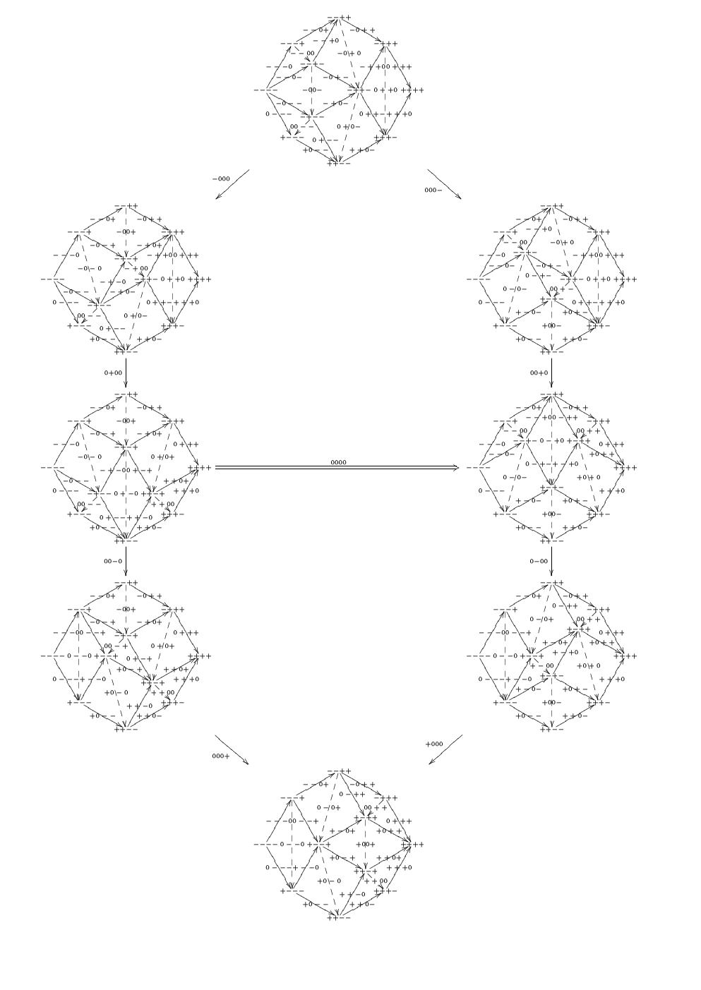
The oriented 44-cube is represented in Figure 14.

00−\scriptstyle{00-}000\scriptstyle{000}+00\scriptstyle{+00}−00\scriptstyle{-00}0+0\scriptstyle{0+0}0−0\scriptstyle{0-0}00+\scriptstyle{00+}
Figure 13: The ω\omega-category I3I^{3}
Refer to caption
Figure 14: The ω\omega-category I4I^{4}

4.2 The cubical singular nerve

The map which sends every ω\omega-category 𝒞\mathcal{C} to 𝒩□​(𝒞)∗=ω​C​a​t​(I∗,𝒞)\mathcal{N}^{\square}(\mathcal{C})_{*}=\omega Cat(I^{*},\mathcal{C}) induces a functor from ω​C​a​t\omega Cat to the category of cubical sets. If xx is an element of ω​C​a​t​(In,𝒞)\omega Cat(I^{n},\mathcal{C}), ϵi​(x)\epsilon_{i}(x) is the ω\omega-functor from In+1I^{n+1} to 𝒞\mathcal{C} defined by ϵi​(x)​(k1​…​kn+1)=x⁡(k1​…​ki^​…​kn+1)\epsilon_{i}(x)(k_{1}...k_{n+1})=x(k_{1}...\widehat{k_{i}}...k_{n+1}) for all ii between 11 and n+1n+1 and ∂iα(x)\partial_{i}^{\alpha}(x) is the ω\omega-functor from In−1I^{n-1} to 𝒞\mathcal{C} defined by ∂iα(x)​(k1​…​kn−1)=x⁡(k1​…​ki−1​α​ki​…​kn−1)\partial_{i}^{\alpha}(x)(k_{1}...k_{n-1})=x(k_{1}...k_{i-1}\alpha k_{i}...k_{n-1}) for all ii between 11 and nn.

The arrow ∂iα\partial_{i}^{\alpha} for a given ii such that 1⩽i⩽n1\leqslant i\leqslant n induces a natural transformation from ω​C​a​t​(In,−)\omega Cat(I^{n},-) to ω​C​a​t​(In−1,−)\omega Cat(I^{n-1},-) and therefore, by Yoneda, corresponds to an ω\omega-functor δiα\delta^{\alpha}_{i} from In−1I^{n-1} to InI^{n}. This functor is defined on the faces of In−1I^{n-1} by δiα​(k1​…​kn−1)=R⁡(k1​…​[α]i​…​kn−1)\delta^{\alpha}_{i}(k_{1}...k_{n-1})=R(k_{1}...[\alpha]_{i}...k_{n-1}). The notation […]i[...]_{i} means that the term inside the brackets are in the ii-th place.

Definition 4.2.

The cubical set ω​C​a​t​(I∗,𝒞)\omega Cat(I^{*},\mathcal{C}) is called the cubical singular nerve of the ω\omega-category 𝒞\mathcal{C}.

This functor is a right adjoint. Its left adjoint is the functor FF.

4.3 Construction of the corner homologies

The starting point is the cubical singular nerve ω​C​a​t​(I∗,𝒞)\omega Cat(I^{*},\mathcal{C}) of 𝒞\mathcal{C} which contains all nn-cubes included in 𝒞\mathcal{C}. The main idea to build the positive and negative corner homology of an ω\omega-category 𝒞\mathcal{C} is to separate the two differential maps ∂−=∑i(−1)i+1∂i−\partial^{-}=\sum_{i}(-1)^{i+1}\partial_{i}^{-} and ∂+=∑i(−1)i+1∂i+\partial^{+}=\sum_{i}(-1)^{i+1}\partial_{i}^{+} and to separately consider the chain complexes of groups (ℤωCat(I∗,𝒞),∂±)(\mathbb{Z}\omega Cat(I^{*},\mathcal{C}),\partial^{\pm}) (a bit as in [Gou95] where the author separates the horizontal and vertical differential maps of a bicomplex). However the following proposition holds :

Proposition 4.2.

Both chain complexes of groups (ℤωCat(I∗,𝒞),∂−)(\mathbb{Z}\omega Cat(I^{*},\mathcal{C}),\partial^{-}) and (ℤωCat(I∗,𝒞),∂+)(\mathbb{Z}\omega Cat(I^{*},\mathcal{C}),\linebreak\partial^{+}) are acyclic.

Proof.

It turns out that ϵ1\epsilon_{1} is a chain retraction of (ℤωCat(I∗,𝒞),∂−)(\mathbb{Z}\omega Cat(I^{*},\mathcal{C}),\partial^{-}). If x∈ℤ​ω​C​a​t​(I0,𝒞)x\in\mathbb{Z}\omega Cat(I^{0},\mathcal{C}), then ∂αϵ1​x=∂1αϵ1​x=x\partial^{\alpha}\epsilon_{1}x=\partial^{\alpha}_{1}\epsilon_{1}x=x. And for x∈ℤ​ω​C​a​t​(In,𝒞)x\in\mathbb{Z}\omega Cat(I^{n},\mathcal{C}), with n⩾1n\geqslant 1, we have actually :

∂α∘ϵ1(x)+ϵ1∘∂α(x)\displaystyle\partial^{\alpha}\circ\epsilon_{1}(x)+\epsilon_{1}\circ\partial^{\alpha}(x) =\displaystyle= ∑i=1i=n+1(−1)i+1​∂iαϵ1​(x)+∑i=1i=n(−1)i+1​ϵ1​∂iα(x)\displaystyle\sum_{i=1}^{i=n+1}(-1)^{i+1}\partial_{i}^{\alpha}\epsilon_{1}(x)+\sum_{i=1}^{i=n}(-1)^{i+1}\epsilon_{1}\partial_{i}^{\alpha}(x)
=\displaystyle= x+∑i=2i=n+1(−1)i+1​ϵ1​∂i−1α(x)+∑i=1i=n(−1)i+1​ϵ1​∂iα(x)\displaystyle x+\sum_{i=2}^{i=n+1}(-1)^{i+1}\epsilon_{1}\partial_{i-1}^{\alpha}(x)+\sum_{i=1}^{i=n}(-1)^{i+1}\epsilon_{1}\partial_{i}^{\alpha}(x)
=\displaystyle= x+∑i=1i=n(−1)i​ϵ1​∂iα(x)+∑i=1i=n(−1)i+1​ϵ1​∂iα(x)\displaystyle x+\sum_{i=1}^{i=n}(-1)^{i}\epsilon_{1}\partial_{i}^{\alpha}(x)+\sum_{i=1}^{i=n}(-1)^{i+1}\epsilon_{1}\partial_{i}^{\alpha}(x)
=\displaystyle= x\displaystyle x

∎

The previous proposition entails the following definition :

Definition 4.3.

Let 𝒞\mathcal{C} be an ω\omega-category and α∈{−,+}\alpha\in\{-,+\}. We denote by ω​C​a​t​(In,𝒞)α\omega Cat(I^{n},\mathcal{C})^{\alpha} the subset of elements xx of ω​C​a​t​(In,𝒞)\omega Cat(I^{n},\mathcal{C}) satisfying the following conditions :

  • •

    the element xx is a non degenerate element of the cubical nerve

  • •

    any element of the form ∂i1α…​∂ipα(x)\partial^{\alpha}_{i_{1}}...\partial^{\alpha}_{i_{p}}(x) is non degenerate in the cubical nerve.

Then ∂α(ℤ​ω​C​a​t​(I∗+1,𝒞)α)⊂ℤ​ω​C​a​t​(I∗,𝒞)α\partial^{\alpha}(\mathbb{Z}\omega Cat(I^{*+1},\mathcal{C})^{\alpha})\subset\mathbb{Z}\omega Cat(I^{*},\mathcal{C})^{\alpha} by construction. We thus set

H∗α(𝒞,ℤ)=H∗(ℤωCat(I∗,𝒞)α,∂α)H_{*}^{\alpha}(\mathcal{C},\mathbb{Z})=H_{*}(\mathbb{Z}\omega Cat(I^{*},\mathcal{C})^{\alpha},\partial^{\alpha})

and we call these homology theories the negative (or positive according to α\alpha) corner homology of 𝒞\mathcal{C}. The cycles are called the negative (or positive) corners of 𝒞\mathcal{C}. The maps H∗±H_{*}^{\pm} induce functors from ω​C​a​t1\omega Cat_{1} to A​bAb.

The second part of the definition is essential. Indeed if aa is a 11-dimensional morphism of 𝒞\mathcal{C}, then the following element of ω​C​a​t​(I2,𝒞)\omega Cat(I^{2},\mathcal{C}) is non degenerate although its image by ∂1−\partial_{1}^{-} and ∂2−\partial_{2}^{-} are degenerate elements of C​a​t​(I1,𝒞)Cat(I^{1},\mathcal{C}) :

s0​(a)\textstyle{s_{0}(a)\ignorespaces\ignorespaces\ignorespaces\ignorespaces\ignorespaces\ignorespaces\ignorespaces\ignorespaces}a\scriptstyle{a}a\scriptstyle{a}t0​(a)\textstyle{t_{0}(a)}s0​(a)\textstyle{s_{0}(a)\ignorespaces\ignorespaces\ignorespaces\ignorespaces\ignorespaces\ignorespaces\ignorespaces\ignorespaces}s0​(a)\scriptstyle{s_{0}(a)}s0​(a)\scriptstyle{s_{0}(a)}s0​(a)\textstyle{s_{0}(a)\ignorespaces\ignorespaces\ignorespaces\ignorespaces}a\scriptstyle{a}

The following proposition characterizes the elements of ω​C​a​t​(I∗,𝒞)α\omega Cat(I^{*},\mathcal{C})^{\alpha}

Proposition 4.3.

Assume that xx is an element of ω​C​a​t​(I∗,𝒞)\omega Cat(I^{*},\mathcal{C}). Then xx is in ω​C​a​t​(I∗,𝒞)α\omega Cat(I^{*},\mathcal{C})^{\alpha} if and only if all x⁡(α​…​0​…​α)x(\alpha...0...\alpha) (the notation α​…​0​…​α\alpha...0...\alpha meaning that 00 appears only once) are 11-dimensional morphisms of 𝒞\mathcal{C}.

Proof.

If xx is in ω​C​a​t​(In,𝒞)α\omega Cat(I^{n},\mathcal{C})^{\alpha}, then all ∂i1α…​∂ipα(x)\partial^{\alpha}_{i_{1}}...\partial^{\alpha}_{i_{p}}(x) are non degenerate in the cubical nerve. But y∈ω​C​a​t​(I1,𝒞)y\in\omega Cat(I^{1},\mathcal{C}) is non degenerate if and only if y⁡(R⁡(0))y(R(0)) is 11-dimensional. Hence the necessity of the condition. Conversely assume that x∉ω​C​a​t​(In,𝒞)αx\notin\omega Cat(I^{n},\mathcal{C})^{\alpha}. Then there exists ii between 11 and nn such that ∂i1α…​∂ipαx=ϵi​(z)\partial^{\alpha}_{i_{1}}...\partial^{\alpha}_{i_{p}}x=\epsilon_{i}(z) with p<np<n and some i1i_{1}, …, ipi_{p} and with z∈ω​C​a​t​(In−p−1,𝒞)z\in\omega Cat(I^{n-p-1},\mathcal{C}). Then

{x⁡(α​…​[−]i​…​α),x⁡(α​…​[0]i​…​α),x⁡(α​…​[+]i​…​α)}\{x(\alpha...[-]_{i}...\alpha),x(\alpha...[0]_{i}...\alpha),x(\alpha...[+]_{i}...\alpha)\}

is a singleton for some ii therefore x⁡(α​…​[0]i​…​α)x(\alpha...[0]_{i}...\alpha) is 00-dimensional. Hence the sufficiency of the condition. ∎

As the globular homology, the corner homologies do not yield functors from ω​C​a​t\omega Cat to A​bAb.

4.4 Examples of corners

Proposition 4.4.

Let 𝒞\mathcal{C} be an ω\omega-category. The group H0−​(𝒞)H_{0}^{-}(\mathcal{C}) is the free abelian group generated by the final states of 𝒞\mathcal{C}. The group H0+​(𝒞)H_{0}^{+}(\mathcal{C}) is the free abelian group generated by the initial states of 𝒞\mathcal{C}.

Proof.

Obvious. ∎

There is in Figure 15 a very simple example of 11-dimensional negative corner. It consists of two ω\omega-functors xx and yy from I1I^{1} to 𝒞\mathcal{C} such that x⁡(R⁡(−))=y⁡(R⁡(−))x(R(-))=y(R(-)) and such that x⁡(R⁡(0))x(R(0)) and y⁡(R⁡(0))y(R(0)) are 11-dimensional. Figure 16 shows an example of 22-dimensional negative corner. If we suppose AA and BB to be oriented such that s1​A=u∗0xs_{1}A=u*_{0}x, t1​A=v∗0yt_{1}A=v*_{0}y, s1​B=u∗0zs_{1}B=u*_{0}z and t1​B=v∗0tt_{1}B=v*_{0}t, then A−BA-B is a negative corner.

Figure 15: A 11-dimensional negative corner
Figure 16: A 22-dimensional negative corner

5 Filling of shells in the cubical singular nerve

Now here is a technical tool which will enable us to construct some operations on the cubical singular nerve of a globular ω\omega-category (Section 6 and Section 10) and to construct the two Hurewicz morphisms (Section 7). The notion of shell and of filling of (thin or not) shells already appears in [BH81b] in the framework of ω\omega-groupoids, in [AA89] in the framework of cubical ω\omega-categories (see Definition 10.1).

5.1 Recall about the freeness of InI^{n}

A key property of InI^{n} is its freeness. It means the following fact. Let pp be some natural number. Let us call a realization (Λp,fi)(\Lambda^{p},f_{i}) of (Λp,E,B)(\Lambda^{p},E,B) in an ω\omega-category 𝒞\mathcal{C} a family of maps fif_{i} from (Λp)i(\Lambda^{p})_{i} to τi​𝒞\tau_{i}\mathcal{C}, where τi​𝒞\tau_{i}\mathcal{C} is the ω\omega-category obtained by only keeping the cells of 𝒞\mathcal{C} of dimension lower or equal than ii. The realization (Λp,fi)(\Lambda^{p},f_{i}) is called nn-extendable if there exists only one functor ff from τn​Ip\tau_{n}I^{p} to 𝒞\mathcal{C} such that for any k⩽nk\leqslant n, the commutative diagram holds

τk​Ip\textstyle{\tau_{k}I^{p}\ignorespaces\ignorespaces\ignorespaces\ignorespaces}τn​Ip\textstyle{\tau_{n}I^{p}\ignorespaces\ignorespaces\ignorespaces\ignorespaces}f\scriptstyle{f}(Λp)k\textstyle{(\Lambda^{p})_{k}\ignorespaces\ignorespaces\ignorespaces\ignorespaces\ignorespaces\ignorespaces\ignorespaces\ignorespaces}R⁡()\scriptstyle{R()}fk\scriptstyle{f_{k}}𝒞\textstyle{{\mathcal{C}}}

By convention, any realization (Λp,fi)(\Lambda^{p},f_{i}) is 00-appropriate and is already 00-extendable since f0f_{0} is already a functor from (Ip)0(I^{p})_{0} to 𝒞\mathcal{C}. Suppose set up a notion of nn-appropriate realization. Then we have

(Λp)n+1\textstyle{(\Lambda^{p})_{n+1}\ignorespaces\ignorespaces\ignorespaces\ignorespaces\ignorespaces\ignorespaces\ignorespaces\ignorespaces}fn+1\scriptstyle{f_{n+1}}R⁡()\scriptstyle{R()}τn+1​Ip\textstyle{\tau_{n+1}I^{p}\ignorespaces\ignorespaces\ignorespaces\ignorespaces\ignorespaces\ignorespaces\ignorespaces\ignorespaces\ignorespaces\ignorespaces\ignorespaces\ignorespaces}tn\scriptstyle{t_{n}}sn\scriptstyle{s_{n}}𝒞\textstyle{{\mathcal{C}}\ignorespaces\ignorespaces\ignorespaces\ignorespaces\ignorespaces\ignorespaces\ignorespaces\ignorespaces}tn\scriptstyle{t_{n}}sn\scriptstyle{s_{n}}τn​Ip\textstyle{\tau_{n}I^{p}\ignorespaces\ignorespaces\ignorespaces\ignorespaces}f\scriptstyle{f}𝒞\textstyle{\mathcal{C}}

A realization (Λp,fi)(\Lambda^{p},f_{i}) is (n+1)(n+1)-appropriate if sn​fn+1=f​sn​Rs_{n}f_{n+1}=fs_{n}R and tn​fn+1=f​tn​Rt_{n}f_{n+1}=ft_{n}R, and in this case, (Λp,fi)(\Lambda^{p},f_{i}) is (n+1)(n+1)-extendable (cf [Joh89] page 224). Thus to construct an ω\omega-functor from InI^{n} for some natural number nn to an ω\omega-category 𝒞\mathcal{C}, it suffices to construct a realization which is appropriate in all dimensions.

5.2 Filling of shells using the freeness of InI^{n}

Definition 5.1.

An element x∈ω​C​a​t​(In,𝒞)x\in\omega Cat(I^{n},\mathcal{C}) is thin if x⁡(R⁡(0n))x(R(0_{n})) is of dimension strictly lower than nn. An element which is not thin is called thick.

Definition 5.2.

A nn-shell in the cubical singular nerve is a family of 2​(n+1)2(n+1) elements xi±x_{i}^{\pm} of ω​C​a​t​(In,𝒞)\omega Cat(I^{n},\mathcal{C}) such that ∂iαxjβ=∂j−1βxiα\partial_{i}^{\alpha}x_{j}^{\beta}=\partial_{j-1}^{\beta}x_{i}^{\alpha} for 1⩽i<j⩽n+11\leqslant i<j\leqslant n+1 and α,β∈{−,+}\alpha,\beta\in\{-,+\}.

Definition 5.3.

The nn-shell (xi±)(x_{i}^{\pm}) is fillable if

  1. 1.

    the sets {xi(−)i,1⩽i⩽n+1}\{x_{i}^{(-)^{i}},1\leqslant i\leqslant n+1\} and {xi(−)i+1,1⩽i⩽n+1}\{x_{i}^{(-)^{i+1}},1\leqslant i\leqslant n+1\} have each one exactly one thick element and if the other ones are thin.

  2. 2.

    if xi0(−)i0x_{i_{0}}^{(-)^{i_{0}}} and xi1(−)i1+1x_{i_{1}}^{(-)^{i_{1}+1}} are these two thick elements then there exists u∈𝒞u\in\mathcal{C} such that sn​(u)=xi0(−)i0​(0n)s_{n}(u)=x_{i_{0}}^{(-)^{i_{0}}}(0_{n}) and tn​(u)=xi1(−)i1+1​(0n)t_{n}(u)=x_{i_{1}}^{(-)^{i_{1}+1}}(0_{n}).

The main proposition of this section is the following one, which is an analogue of [AA89] Proposition 2.7.3.

Proposition 5.1.

Let (xi±)(x_{i}^{\pm}) be a fillable nn-shell with uu as above. Then there exists one and only one element xx of ω​C​a​t​(In+1,𝒞)\omega Cat(I^{n+1},\mathcal{C}) such that x⁡(0n+1)=ux(0_{n+1})=u, and for 1⩽i⩽n+11\leqslant i\leqslant n+1, and α∈{−,+}\alpha\in\{-,+\} such that ∂iαx=xiα\partial_{i}^{\alpha}x=x_{i}^{\alpha}.

Proof.

The underlying idea of the proof is as follows. If one wants to define an ω\omega-functor from In+1I^{n+1} to an ω\omega-category 𝒞\mathcal{C}, it suffices to construct 2​(n+1)2(n+1) ω\omega-functors from the 2​(n+1)2(n+1) nn-faces of In+1I^{n+1} to 𝒞\mathcal{C} which coincide on the intersection of their definition domains and to fill correctly the interior of In+1I^{n+1}.

We have necessarily x⁡(k1​…​[±]i​…​kn)=xi±​(k1​…​kn)x(k_{1}\dots[\pm]_{i}\dots k_{n})=x_{i}^{\pm}(k_{1}...k_{n}) and x⁡(0n+1)=ux(0_{n+1})=u. Therefore there is at most one such realization (Λn+1,xi)(\Lambda^{n+1},x_{i}). It suffices to show that xx is (n+1)(n+1)-extendable. It is certainly 00-appropriate therefore 00-extendable. Suppose we have proved that this realization is pp-appropriate and therefore pp-extendable for every p<n+1p<n+1. First suppose that p<np<n. We want to prove that (Λn+1,xi)(\Lambda^{n+1},x_{i}) is (p+1)(p+1)-appropriate, i.e. that sp​x​(k1​…​kn+1)=x​sp​R​(k1​…​kn+1)s_{p}x(k_{1}\dots k_{n+1})=xs_{p}R(k_{1}\dots k_{n+1}) and tp​x​(k1​…​kn+1)=x​tp​R​(k1​…​kn+1)t_{p}x(k_{1}\dots k_{n+1})=xt_{p}R(k_{1}\dots k_{n+1}) for k1​…​kn+1k_{1}\dots k_{n+1} of dimension p+1p+1.

Let us verify the first equality. We have

sp​x​(k1​…​kn+1)\displaystyle s_{p}x(k_{1}\dots k_{n+1}) =\displaystyle= sp​(∂ikix)​(k1​…​ki^​…​kn+1)​ since p+1<n+1\displaystyle s_{p}(\partial_{i}^{k_{i}}x)(k_{1}\dots\widehat{k_{i}}\dots k_{n+1})\hbox{ since $p+1<n+1$}
=\displaystyle= sp​xiki​(k1​…​ki^​…​kn+1)\displaystyle s_{p}x_{i}^{k_{i}}(k_{1}\dots\widehat{k_{i}}\dots k_{n+1})
=\displaystyle= xiki​sp​R​(k1​…​ki^​…​kn+1)​ since the xiα are ω-functors\displaystyle x_{i}^{k_{i}}s_{p}R(k_{1}\dots\widehat{k_{i}}\dots k_{n+1})\hbox{ since the $x_{i}^{\alpha}$ are $\omega$-functors}

But sp​R​(k1​…​ki^​…​kn+1)=Ψ⁡(R⁡(X1),…,R⁡(Xs))s_{p}R(k_{1}\dots\widehat{k_{i}}\dots k_{n+1})=\Psi(R(X_{1}),...,R(X_{s})) where Ψ\Psi consists only of compositions of XhX_{h} of dimension lower than pp. Then

sp​x​(k1​…​kn+1)\displaystyle s_{p}x(k_{1}\dots k_{n+1}) =\displaystyle= Ψ⁡(xiki​R​(X1),…,xiki​R​(Xs))\displaystyle\Psi(x_{i}^{k_{i}}R(X_{1}),...,x_{i}^{k_{i}}R(X_{s}))
=\displaystyle= Ψ⁡((∂ikix)​R​(X1),…,(∂ikix)​R​(Xs))\displaystyle\Psi((\partial_{i}^{k_{i}}x)R(X_{1}),...,(\partial_{i}^{k_{i}}x)R(X_{s}))
=\displaystyle= x​Ψ​(δiki​R​(X1),…,δiki​R​(Xs))​ since x is p-extendable\displaystyle x\Psi(\delta_{i}^{k_{i}}R(X_{1}),...,\delta_{i}^{k_{i}}R(X_{s}))\hbox{ since $x$ is $p$-extendable}
=\displaystyle= x​sp​R​(k1​…​kn+1)​ since δiki is an ω-functor\displaystyle xs_{p}R(k_{1}\dots k_{n+1})\hbox{ since $\delta_{i}^{k_{i}}$ is an $\omega$-functor}

It remains to prove that xx is (n+1)(n+1)-extendable. We have to prove that sn​x​(0n+1)=x​sn​R​(0n+1)s_{n}x(0_{n+1})=xs_{n}R(0_{n+1}) and tn​x​(0n+1)=x​tn​R​(0n+1)t_{n}x(0_{n+1})=xt_{n}R(0_{n+1}). Let us verify the first equality. We have sn​R​(0n+1)=Ψ′​(δi0(−)i0​(0n),Y1,…,Ys)s_{n}R(0_{n+1})=\Psi^{\prime}(\delta_{i_{0}}^{(-)^{i_{0}}}(0_{n}),Y_{1},\dots,Y_{s}) where Ψ′\Psi^{\prime} is a function containing only composition maps and where Y1,…,YsY_{1},\dots,Y_{s} are elements of In+1I^{n+1} of the form R⁡({x})R(\{x\}) where xx is a face of the (n+1)(n+1)-cube. Then

x​sn​R​(0n+1)\displaystyle xs_{n}R(0_{n+1}) =\displaystyle= x​Ψ′​(δi0(−)i0​(0n),Y1,…,Ys)\displaystyle x\Psi^{\prime}(\delta_{i_{0}}^{(-)^{i_{0}}}(0_{n}),Y_{1},\dots,Y_{s})
=\displaystyle= Ψ′​(x⁡(δi0(−)i0​(0n)),x⁡(Y1),…,x⁡(Ys))​ since x is n-extendable\displaystyle\Psi^{\prime}(x(\delta_{i_{0}}^{(-)^{i_{0}}}(0_{n})),x(Y_{1}),\dots,x(Y_{s}))\hbox{ since $x$ is $n$-extendable}
=\displaystyle= x⁡(δi0(−)i0​(0n))​ since d​i​m​(x⁡(Y1)),…,d​i​m​(x⁡(Ys))<n\displaystyle x(\delta_{i_{0}}^{(-)^{i_{0}}}(0_{n}))\hbox{ since $dim(x(Y_{1})),\dots,dim(x(Y_{s}))<n$}
=\displaystyle= xi0(−)i0​(0n)\displaystyle x_{i_{0}}^{(-)^{i_{0}}}(0_{n})
=\displaystyle= sn​(u)​ by definition of u\displaystyle s_{n}(u)\hbox{ by definition of $u$}
=\displaystyle= sn​x​(0n+1)​ by definition of x\displaystyle s_{n}x(0_{n+1})\hbox{ by definition of $x$}

∎

6 Two new simplicial nerves

As an immediate application of Section 5 , we construct two families of connections on the cubical singular nerve of any ω\omega-category. They will be useful in the sequel.

6.1 Cubical set with connections

Definition 6.1.

[AA89] A cubical set with connections consists of a cubical set

((Kn)n⩾0,∂iα,ϵi)((K_{n})_{n\geqslant 0},\partial_{i}^{\alpha},\epsilon_{i})

together with two additional families of degeneracy maps

Γiα:    Kn          Kn+1    \Gamma_{i}^{\alpha}:\lx@xy@svg{\hbox{\raise 2.55554pt\hbox{\kern 10.32582pt\hbox{\ignorespaces\ignorespaces\ignorespaces\hbox{\vtop{\halign{\entry@#!@&&\entry@@#!@\cr&\crcr}}}\ignorespaces{\hbox{\kern-10.32582pt\raise 0.0pt\hbox{\hbox{\kern 0.0pt\raise 0.0pt\hbox{\hbox{\kern 3.0pt\raise-2.55554pt\hbox{$\textstyle{K_{n}\ignorespaces\ignorespaces\ignorespaces\ignorespaces}$}}}}}}}\ignorespaces\ignorespaces\ignorespaces\ignorespaces{}{\hbox{\lx@xy@droprule}}\ignorespaces\ignorespaces{\hbox{\kern 21.85709pt\raise 0.0pt\hbox{{}\hbox{\kern 0.0pt\raise 0.0pt\hbox{\hbox{\kern 3.0pt\hbox{\hbox{\kern 0.0pt\raise 0.0pt\hbox{$\scriptstyle{}$}}}\kern 3.0pt}}}}}}\ignorespaces{\hbox{\kern 34.32582pt\raise 0.0pt\hbox{\hbox{\kern 0.0pt\raise 0.0pt\hbox{\lx@xy@tip{1}\lx@xy@tip{-1}}}}}}{\hbox{\lx@xy@droprule}}{\hbox{\lx@xy@droprule}}{\hbox{\kern 34.32582pt\raise 0.0pt\hbox{\hbox{\kern 0.0pt\raise 0.0pt\hbox{\hbox{\kern 3.0pt\raise-2.55554pt\hbox{$\textstyle{K_{n+1}}$}}}}}}}\ignorespaces}}}}\ignorespaces

with α∈{−,+}\alpha\in\{-,+\}, n⩾1n\geqslant 1 and 1⩽i⩽n1\leqslant i\leqslant n and satisfying the following axioms :

  1. 1.

    ∂iαΓjβ=Γβj−1∂iα\partial_{i}^{\alpha}\Gamma_{j}^{\beta}=\Gamma^{\beta}_{j-1}\partial_{i}^{\alpha} for all i<ji<j and all α,β∈{−,+}\alpha,\beta\in\{-,+\}

  2. 2.

    ∂iαΓjβ=Γβj∂i−1α\partial_{i}^{\alpha}\Gamma_{j}^{\beta}=\Gamma^{\beta}_{j}\partial_{i-1}^{\alpha} for all i>j+1i>j+1 and all α,β∈{−,+}\alpha,\beta\in\{-,+\}

  3. 3.

    ∂j±Γj±=∂j+1±Γj±=I​d\partial_{j}^{\pm}\Gamma_{j}^{\pm}=\partial_{j+1}^{\pm}\Gamma_{j}^{\pm}=Id

  4. 4.

    ∂j±Γj∓=∂j+1±Γj∓=ϵj∂j±\partial_{j}^{\pm}\Gamma_{j}^{\mp}=\partial_{j+1}^{\pm}\Gamma_{j}^{\mp}=\epsilon_{j}\partial_{j}^{\pm}

  5. 5.

    Γi±​Γj±=Γj+1±​Γi±\Gamma_{i}^{\pm}\Gamma_{j}^{\pm}=\Gamma_{j+1}^{\pm}\Gamma_{i}^{\pm} if i⩽ji\leqslant j

  6. 6.

    Γi±​Γj∓=Γj+1∓​Γi±\Gamma_{i}^{\pm}\Gamma_{j}^{\mp}=\Gamma_{j+1}^{\mp}\Gamma_{i}^{\pm} if i<ji<j

  7. 7.

    Γi±​Γj∓=Γj∓​Γi−1±\Gamma_{i}^{\pm}\Gamma_{j}^{\mp}=\Gamma_{j}^{\mp}\Gamma_{i-1}^{\pm} if i>j+1i>j+1

  8. 8.

    Γi±​ϵj=ϵj+1​Γi±\Gamma_{i}^{\pm}\epsilon_{j}=\epsilon_{j+1}\Gamma_{i}^{\pm} if i<ji<j

  9. 9.

    Γi±​ϵj=ϵi​ϵi\Gamma_{i}^{\pm}\epsilon_{j}=\epsilon_{i}\epsilon_{i} if i=ji=j

  10. 10.

    Γi±​ϵj=ϵj​Γi−1±\Gamma_{i}^{\pm}\epsilon_{j}=\epsilon_{j}\Gamma_{i-1}^{\pm} if i>ji>j

There is an obviously defined small category Γ\Gamma, such that the category of cubical sets with connections is exactly the category of presheaves over Γ\Gamma. Hence the category of cubical set with connections is denoted by S​e​t​sΓo​pSets^{\Gamma^{op}}.

The category of cubical sets with connections equipped with the non 11-contracting morphisms is denoted by S​e​t​s1Γo​pSets_{1}^{\Gamma^{op}}.

Looking back to the cubical singular nerve of a topological space, we can endow it with connections as follows :

Γi−​(f)​(x1,…,xp)=f⁡(x1,…,m​a​x​(xi,xi+1),…,xp)\displaystyle\Gamma_{i}^{-}(f)(x_{1},\dots,x_{p})=f(x_{1},\dots,max(x_{i},x_{i+1}),\dots,x_{p})
Γi+​(f)​(x1,…,xp)=f⁡(x1,…,m​i​n​(xi,xi+1),…,xp)\displaystyle\Gamma_{i}^{+}(f)(x_{1},\dots,x_{p})=f(x_{1},\dots,min(x_{i},x_{i+1}),\dots,x_{p})

By keeping in a cubical set with connections only the morphisms Γi−\Gamma_{i}^{-}, or by exchanging the role of the face maps ∂i+\partial_{i}^{+} and ∂i−\partial_{i}^{-} and by keeping only the morphisms Γi+\Gamma_{i}^{+}, we obtain exactly a cubical set with connections in the sense of Brown-Higgins.

6.2 Construction of connections on the cubical singular nerve

Theorem 6.1.

Let 𝒞\mathcal{C} be an ω\omega-category and let nn be a natural number greater or equal than 11. For any xx in ω​C​a​t​(In,𝒞)\omega Cat(I^{n},\mathcal{C}) and for any ii between 11 and nn, we introduce two realizations Γi−​(x)\Gamma_{i}^{-}(x) and Γi+​(x)\Gamma_{i}^{+}(x) from Λn+1\Lambda^{n+1} to 𝒞\mathcal{C} by setting

Γi−​(x)​(k1​…​kn+1)=x⁡(k1​…​m​a​x​(ki,ki+1)​…​kn+1)\displaystyle\Gamma_{i}^{-}(x)(k_{1}...k_{n+1})=x(k_{1}...max(k_{i},k_{i+1})...k_{n+1})
Γi+​(x)​(k1​…​kn+1)=x⁡(k1​…​m​i​n​(ki,ki+1)​…​kn+1)\displaystyle\Gamma_{i}^{+}(x)(k_{1}...k_{n+1})=x(k_{1}...min(k_{i},k_{i+1})...k_{n+1})

where the set {−,0,+}\{-,0,+\} is ordered by −<0<+-<0<+. Then Γi−​(x)\Gamma_{i}^{-}(x) and Γi+​(x)\Gamma_{i}^{+}(x) yield ω\omega-functors from In+1I^{n+1} to 𝒞\mathcal{C}, meaning two elements of ω​C​a​t​(In+1,𝒞)\omega Cat(I^{n+1},\mathcal{C}). Moreover, in this way, the cubical nerve of 𝒞\mathcal{C} is equipped with a structure of cubical complex with connections.

Proof.

The construction of Γi±\Gamma_{i}^{\pm} is exactly the same as the one of connections on the cubical singular nerve of a topological space. Thus there is nothing to verify in the axioms of cubical complex with connections except the relations mixing the two families of degeneracies Γi+\Gamma_{i}^{+} and Γi−\Gamma_{i}^{-} : all other axioms are already verified in [BH81b]. Therefore it remains to verify that Γi±​Γj∓=Γj+1∓​Γi±\Gamma_{i}^{\pm}\Gamma_{j}^{\mp}=\Gamma_{j+1}^{\mp}\Gamma_{i}^{\pm} if i<ji<j, and Γi±​Γj∓=Γj∓​Γi−1±\Gamma_{i}^{\pm}\Gamma_{j}^{\mp}=\Gamma_{j}^{\mp}\Gamma_{i-1}^{\pm} if i>j+1i>j+1, that can be done quickly. The only remaining point to be verified is that all realizations Γi±​(x)\Gamma_{i}^{\pm}(x) yield ω\omega-functors.

If xx is an element of ω​C​a​t​(I1,𝒞)\omega Cat(I^{1},\mathcal{C}), then we can depict Γ1−​(x)\Gamma_{1}^{-}(x) as in Figure 17 and Γ1+​(x)\Gamma_{1}^{+}(x) as in Figure 18. We see immediately that Γ1−​(x)\Gamma_{1}^{-}(x) and Γ1+​(x)\Gamma_{1}^{+}(x) yield two elements of ω​C​a​t​(I2,𝒞)\omega Cat(I^{2},\mathcal{C}).

x⁡(+)\textstyle{x(+)\ignorespaces\ignorespaces\ignorespaces\ignorespaces\ignorespaces\ignorespaces\ignorespaces\ignorespaces}x⁡(+)\scriptstyle{x(+)}x⁡(0)\scriptstyle{x(0)}x⁡(+)\textstyle{x(+)}x⁡(−)\textstyle{x(-)\ignorespaces\ignorespaces\ignorespaces\ignorespaces\ignorespaces\ignorespaces\ignorespaces\ignorespaces}x⁡(0)\scriptstyle{x(0)}x⁡(0)\scriptstyle{x(0)}x⁡(+)\textstyle{x(+)\ignorespaces\ignorespaces\ignorespaces\ignorespaces}x⁡(+)\scriptstyle{x(+)}
Figure 17: Γ1−​(x)\Gamma_{1}^{-}(x)
x⁡(−)\textstyle{x(-)\ignorespaces\ignorespaces\ignorespaces\ignorespaces\ignorespaces\ignorespaces\ignorespaces\ignorespaces}x⁡(0)\scriptstyle{x(0)}x⁡(0)\scriptstyle{x(0)}x⁡(+)\textstyle{x(+)}x⁡(−)\textstyle{x(-)\ignorespaces\ignorespaces\ignorespaces\ignorespaces\ignorespaces\ignorespaces\ignorespaces\ignorespaces}x⁡(−)\scriptstyle{x(-)}x⁡(−)\scriptstyle{x(-)}x⁡(−)\textstyle{x(-)\ignorespaces\ignorespaces\ignorespaces\ignorespaces}x⁡(0)\scriptstyle{x(0)}
Figure 18: Γ1+​(x)\Gamma_{1}^{+}(x)

Suppose we have proved that all realizations Γi±​(x)\Gamma_{i}^{\pm}(x) for 1⩽i⩽n1\leqslant i\leqslant n yield ω\omega-functors if x∈ω​C​a​t​(In,𝒞)x\in\omega Cat(I^{n},\mathcal{C}). Now we want to prove that all realizations Γi±​(y)\Gamma_{i}^{\pm}(y) for 1⩽i⩽n+11\leqslant i\leqslant n+1 yield ω\omega-functors if y∈ω​C​a​t​(In+1,𝒞)y\in\omega Cat(I^{n+1},\mathcal{C}).

Because of the axioms of cubical set with connections and because of the induction hypothesis, the (∂jαΓi±​(y))(\partial_{j}^{\alpha}\Gamma_{i}^{\pm}(y)) are ω\omega-functor from InI^{n} to 𝒞\mathcal{C}. The family (∂jαΓi±​(y))(\partial_{j}^{\alpha}\Gamma_{i}^{\pm}(y)) is also a nn-shell. We can fill it in a canonical way because the top dimensional elements are the same. ∎

We denote by S​e​t​sΔo​pSets^{\Delta^{op}} the category of simplicial sets [May67]. If AA is a simplicial set, the axioms of simplicial sets imply that C(A)=(ℤA∗,∂=∑(−1)i∂i)C(A)=(\mathbb{Z}A_{*},\partial=\sum(-1)^{i}\partial_{i}), where ℤ​An\mathbb{Z}A_{n} means the free abelian group generated by the set AnA_{n}, is a chain complex. It is called the unnormalized chain complex of AA. The normalized chain complex of AA is the quotient chain complex N⁡(A)=C⁡(A)/D⁡(A)N(A)=C(A)/D(A) where D⁡(A)D(A) is the sub-complex of C⁡(A)C(A) generated by the degenerate elements. It turns out that the canonical morphism of chain complex from C⁡(A)C(A) to N⁡(A)N(A) is a quasi-isomorphism [Wei94].

As a consequence of the previous construction, we obtain two new simplicial nerves.

Proposition 6.2.

Let 𝒞\mathcal{C} be an ω\omega-category and α∈{−,+}\alpha\in\{-,+\}. We set

𝒩nα​(𝒞)=ω​C​a​t​(In+1,𝒞)α\mathcal{N}^{\alpha}_{n}(\mathcal{C})=\omega Cat(I^{n+1},\mathcal{C})^{\alpha}

and for all n⩾0n\geqslant 0 and all 0⩽i⩽n0\leqslant i\leqslant n,

∂i:𝒩nα​(𝒞)\textstyle{{\partial_{i}:\mathcal{N}^{\alpha}_{n}(\mathcal{C})}\ignorespaces\ignorespaces\ignorespaces\ignorespaces}𝒩n−1α​(𝒞)\textstyle{\mathcal{N}^{\alpha}_{n-1}(\mathcal{C})}

is the arrow ∂i+1α\partial^{\alpha}_{i+1}, and

ϵi:𝒩nα​(𝒞)\textstyle{{\epsilon_{i}:\mathcal{N}^{\alpha}_{n}(\mathcal{C})}\ignorespaces\ignorespaces\ignorespaces\ignorespaces}𝒩n+1α​(𝒞)\textstyle{\mathcal{N}^{\alpha}_{n+1}(\mathcal{C})}

is the arrow Γi+1α\Gamma^{\alpha}_{i+1}. We obtain this way a simplicial set

(𝒩∗α(𝒞),∂i,ϵi)(\mathcal{N}^{\alpha}_{*}(\mathcal{C}),\partial_{i},\epsilon_{i})

called the negative (or positive according to α\alpha) corner simplicial nerve of 𝒞\mathcal{C}. The non normalized chain complex associated to it gives exactly the corner homology of 𝒞\mathcal{C} (in degree greater than or equal to 11). The maps 𝒩α\mathcal{N}^{\alpha} induces a functor from ω​C​a​t1\omega Cat_{1} to S​e​t​sΔo​pSets^{\Delta^{op}}.

Proof.

The axioms of simplicial sets are immediate consequences of the axioms of cubical set with connections. ∎

Notice that the indices are shifted by one. Intuitively, these simplicial nerves consist of cutting an oriented nn-hypercube by an hyperplane close to a corner (the negative one or the positive one) : the intersection we get is the oriented (n−1)(n-1)-simplex in sense of [Str87].

7 The oriented Hurewicz morphisms

In this section, we construct natural morphisms from the globular homology of a ω\omega-category 𝒞\mathcal{C} to its two corner homology theories. We call these maps the negative and positive oriented Hurewicz morphisms. Intuitively, they map any oriented loop with corners to its corresponding negative or positive corners (except for the 00-dimensional, see below).

7.1 The 00-dimensional case

The projection from ℤ​𝒞0×ℤ​𝒞0\mathbb{Z}\mathcal{C}_{0}\times\mathbb{Z}\mathcal{C}_{0} to ℤ​𝒞0\mathbb{Z}\mathcal{C}_{0} on the first (resp. the second) component yields a natural group morphism from H0g​l​(𝒞)H_{0}^{gl}(\mathcal{C}) to H0−​(𝒞)H_{0}^{-}(\mathcal{C}) (resp. H0+​(𝒞)H_{0}^{+}(\mathcal{C})). Indeed if

X=(s0​(x−y),t0​(x−y)),X=(s_{0}(x-y),t_{0}(x-y)),

then the first component (resp. the second one) of XX induces 00 on the corner homology. We obtain thus a natural morphism h0±h_{0}^{\pm} from H0g​l​(𝒞)H_{0}^{gl}(\mathcal{C}) to H0±​(𝒞)H_{0}^{\pm}(\mathcal{C}).

7.2 The 11-dimensional case

If xx is a 11-dimensional morphism of 𝒞\mathcal{C}, let □1​(x)\square_{1}(x) be the element of ω​C​a​t​(I1,𝒞)\omega Cat(I^{1},\mathcal{C}) defined by

□1​(x)​(R⁡(−))=s0​(x),□1​(x)​(R⁡(0))=x,□1​(x)​(R⁡(+))=t0​(x).\square_{1}(x)(R(-))=s_{0}(x),\square_{1}(x)(R(0))=x,\square_{1}(x)(R(+))=t_{0}(x).

We extend □1\square_{1} by linearity. If zz is a 22-dimensional morphism of 𝒞\mathcal{C}, let □2−​(z)\square^{-}_{2}(z) be the element of ω​C​a​t​(I2,𝒞)\omega Cat(I^{2},\mathcal{C}) defined by the diagram

t0​(z)\textstyle{t_{0}(z)\ignorespaces\ignorespaces\ignorespaces\ignorespaces\ignorespaces\ignorespaces\ignorespaces\ignorespaces}t0​(z)\scriptstyle{t_{0}(z)}z\scriptstyle{z}t0​(z)\textstyle{t_{0}(z)}s0​(z)\textstyle{s_{0}(z)\ignorespaces\ignorespaces\ignorespaces\ignorespaces\ignorespaces\ignorespaces\ignorespaces\ignorespaces}s1​(z)\scriptstyle{s_{1}(z)}t1​(z)\scriptstyle{t_{1}(z)}t0​(z)\textstyle{t_{0}(z)\ignorespaces\ignorespaces\ignorespaces\ignorespaces}t0​(z)\scriptstyle{t_{0}(z)}

and let □2+​(z)\square^{+}_{2}(z) be the element of ω​C​a​t​(I2,𝒞)\omega Cat(I^{2},\mathcal{C}) defined by

s0​(z)\textstyle{s_{0}(z)\ignorespaces\ignorespaces\ignorespaces\ignorespaces\ignorespaces\ignorespaces\ignorespaces\ignorespaces}s1​(z)\scriptstyle{s_{1}(z)}z\scriptstyle{z}t0​(z)\textstyle{t_{0}(z)}s0​(z)\textstyle{s_{0}(z)\ignorespaces\ignorespaces\ignorespaces\ignorespaces\ignorespaces\ignorespaces\ignorespaces\ignorespaces}s0​(z)\scriptstyle{s_{0}(z)}s0​(z)\scriptstyle{s_{0}(z)}s0​(z)\textstyle{s_{0}(z)\ignorespaces\ignorespaces\ignorespaces\ignorespaces}t1​(z)\scriptstyle{t_{1}(z)}

We extend □2−​()\square^{-}_{2}() and □2+​()\square^{+}_{2}() by linearity. We get thus the following proposition

Proposition 7.1.

The natural linear map h1±h_{1}^{\pm} from ℤ​𝒞1\mathbb{Z}\mathcal{C}_{1} to ℤ​ω​C​a​t​(I1,𝒞)±\mathbb{Z}\omega Cat(I^{1},\mathcal{C})^{\pm} which maps x1x_{1} to □1​(x1)\square_{1}(x_{1}) induces a natural map (still denoted by h1±h_{1}^{\pm}) from H1g​l​(𝒞)H_{1}^{gl}(\mathcal{C}) to H1±​(𝒞)H_{1}^{\pm}(\mathcal{C}). We call it the 11-dimensional oriented Hurewicz morphism.

Proof.

The proof is quite simple. If x1x_{1} is a 11-dimensional globular cycle, then

∂±□1​(x1)=□1​(x1)​(±)=0\partial^{\pm}\square_{1}(x_{1})=\square_{1}(x_{1})(\pm)=0

because of the definition of □1​(x1)\square_{1}(x_{1}). And a 11-dimensional globular boundary s1​(x2)−t1​(x2)s_{1}(x_{2})-t_{1}(x_{2}) is mapped to ∂±(□2−​(x2))\partial^{\pm}(\square_{2}^{-}(x_{2})). ∎

7.3 The higher dimensional case

Proposition 7.2.

For any natural number nn greater or equal than 22, there exists a unique natural map □n−\square_{n}^{-} from 𝒞n\mathcal{C}_{n} (the nn-dimensional cells of 𝒞\mathcal{C}) to ω​C​a​t​(In,𝒞)\omega Cat(I^{n},\mathcal{C}) such that

  1. 1.

    the equality □n−​(x)​(0n)=x\square_{n}^{-}(x)(0_{n})=x holds.

  2. 2.

    if n⩾3n\geqslant 3 and 1⩽i⩽n−21\leqslant i\leqslant n-2, then ∂i±□n−=Γn−2−​∂i±□n−1−​sn−1\partial_{i}^{\pm}\square_{n}^{-}=\Gamma_{n-2}^{-}\partial_{i}^{\pm}\square^{-}_{n-1}s_{n-1}.

  3. 3.

    if n⩾2n\geqslant 2 and n−1⩽i⩽nn-1\leqslant i\leqslant n, then ∂i−□n−=□n−1−​dn−1(−)i\partial_{i}^{-}\square_{n}^{-}=\square_{n-1}^{-}d_{n-1}^{(-)^{i}} and ∂i+□n−=ϵn−1​∂n−1+□n−1−​sn−1\partial_{i}^{+}\square_{n}^{-}=\epsilon_{n-1}\partial_{n-1}^{+}\square_{n-1}^{-}s_{n-1}.

Moreover for 1⩽i⩽n1\leqslant i\leqslant n, we have ∂i±□n−​sn​u=∂i±□n−​tn​u\partial_{i}^{\pm}\square_{n}^{-}s_{n}u=\partial_{i}^{\pm}\square_{n}^{-}t_{n}u for any (n+1)(n+1)-morphism uu.

Proof.

Let k1​…​kn−1∈Λn−1k_{1}\dots k_{n-1}\in\Lambda^{n-1}. Then the natural map e​vk1​…​kn−1​∂i±□n−ev_{k_{1}\dots k_{n-1}}\partial_{i}^{\pm}\square_{n}^{-} from 𝒞n\mathcal{C}_{n} to 𝒞n−1\mathcal{C}_{n-1} which sends x∈𝒞nx\in\mathcal{C}_{n} to (∂i±□n−​x)​(k1​…​kn−1)(\partial_{i}^{\pm}\square_{n}^{-}x)(k_{1}\dots k_{n-1}) corresponds by Yoneda to an ω\omega-functor fk1​…​kn−1f_{k_{1}\dots k_{n-1}} from 2n−12_{n-1} to 2n2_{n}, where 2n−12_{n-1} (resp. 2n2_{n}) is the free ω\omega-category generated by a (n−1)(n-1)-morphism AA (resp. a nn-morphism BB). Set

fk1​…​kn−1​(A)=dnk1​…​kn−1αk1​…​kn−1​(B)f_{k_{1}\dots k_{n-1}}(A)=d_{n_{k_{1}\dots k_{n-1}}}^{\alpha_{k_{1}\dots k_{n-1}}}(B)

with still the convention d−=sd^{-}=s and d+=td^{+}=t. Then fk1​…​kn−1=dnk1​…​kn−1αk1​…​kn−1f_{k_{1}\dots k_{n-1}}=d_{n_{k_{1}\dots k_{n-1}}}^{\alpha_{k_{1}\dots k_{n-1}}} because of the freeness of 2n−12_{n-1}. Moreover, the inequality nk1​…​kn−1⩽n−1n_{k_{1}\dots k_{n-1}}\leqslant n-1 holds. Therefore

(∂i±□n−​sn​u)​(k1​…​kn−1)\displaystyle(\partial_{i}^{\pm}\square_{n}^{-}s_{n}u)(k_{1}\dots k_{n-1}) =\displaystyle= dnk1​…​kn−1αk1​…​kn−1​sn​u\displaystyle d_{n_{k_{1}\dots k_{n-1}}}^{\alpha_{k_{1}\dots k_{n-1}}}s_{n}u
=\displaystyle= dnk1​…​kn−1αk1​…​kn−1​tn​u\displaystyle d_{n_{k_{1}\dots k_{n-1}}}^{\alpha_{k_{1}\dots k_{n-1}}}t_{n}u
=\displaystyle= (∂i±□n−​tn​u)​(k1​…​kn−1)\displaystyle(\partial_{i}^{\pm}\square_{n}^{-}t_{n}u)(k_{1}\dots k_{n-1})

Therefore for 1⩽i⩽n1\leqslant i\leqslant n, we have ∂i±□n−​sn​u=∂i±□n−​tn​u\partial_{i}^{\pm}\square_{n}^{-}s_{n}u=\partial_{i}^{\pm}\square_{n}^{-}t_{n}u for any (n+1)(n+1)-morphism uu.

Suppose the proposition proved for p<np<n with n⩾2n\geqslant 2 and take a nn-dimensional morphism xx. Set hi±=Γn−2−​∂i±□n−1−​sn−1​(x)h_{i}^{\pm}=\Gamma_{n-2}^{-}\partial_{i}^{\pm}\square^{-}_{n-1}{s_{n-1}(x)} for 1⩽i⩽n−21\leqslant i\leqslant n-2, and set hi−=□n−1−​dn−1(−)i​xh_{i}^{-}=\square^{-}_{n-1}{d_{n-1}^{(-)^{i}}x} and hi+=ϵn−1​∂n−1+□n−1−​sn−1​(x)h_{i}^{+}=\epsilon_{n-1}\partial_{n-1}^{+}\square^{-}_{n-1}{s_{n-1}(x)} for i⩾n−1i\geqslant n-1. We are going to verify that (hi±)(h_{i}^{\pm}) is a fillable (n−1)(n-1)-shell. It is sufficient to prove that for any ii and any jj between 11 and nn, and any α,β∈{−,+}\alpha,\beta\in\{-,+\}, the equality ∂iαhjβ=∂j−1βhiα\partial_{i}^{\alpha}h_{j}^{\beta}=\partial_{j-1}^{\beta}h_{i}^{\alpha} holds as soon as 1⩽i<j⩽n1\leqslant i<j\leqslant n.

First treat the case i<j⩽n−2i<j\leqslant n-2. We have

∂iαhjβ\displaystyle\partial_{i}^{\alpha}h_{j}^{\beta} =\displaystyle= ∂iαΓn−2−​∂jβ□n−1−​sn−1​(x)​ since j<n−1\displaystyle\partial_{i}^{\alpha}\Gamma_{n-2}^{-}\partial_{j}^{\beta}\square^{-}_{n-1}{s_{n-1}(x)}\hbox{ since $j<n-1$}
=\displaystyle= Γn−3−​∂iα∂jβ□n−1−​sn−1​(x)​ since i<n−2\displaystyle\Gamma_{n-3}^{-}\partial_{i}^{\alpha}\partial_{j}^{\beta}\square^{-}_{n-1}{s_{n-1}(x)}\hbox{ since $i<n-2$}
=\displaystyle= Γn−3−​∂j−1β∂iα□n−1−​sn−1​(x)\displaystyle\Gamma_{n-3}^{-}\partial_{j-1}^{\beta}\partial_{i}^{\alpha}\square^{-}_{n-1}{s_{n-1}(x)}
=\displaystyle= ∂j−1βhiα​ since i<n−1\displaystyle\partial_{j-1}^{\beta}h_{i}^{\alpha}\hbox{ since $i<n-1$}

Now treat the case i<j=n−1i<j=n-1. We have

∂i±hj−\displaystyle\partial_{i}^{\pm}h_{j}^{-} =\displaystyle= ∂i±□n−1−​dn−1(−)n−1​x\displaystyle\partial_{i}^{\pm}\square^{-}_{n-1}{d_{n-1}^{(-)^{n-1}}x}
=\displaystyle= ∂j−1−Γn−2−​∂i±□n−1−​dn−1(−)n−1​x\displaystyle\partial_{j-1}^{-}\Gamma_{n-2}^{-}\partial_{i}^{\pm}\square^{-}_{n-1}{d_{n-1}^{(-)^{n-1}}x}
=\displaystyle= ∂j−1−hi±\displaystyle\partial_{j-1}^{-}h_{i}^{\pm}

We have also

∂i±hn−1+\displaystyle\partial_{i}^{\pm}h_{n-1}^{+} =\displaystyle= ∂i±ϵn−1​∂n−1+□n−1−​sn−1​(x)\displaystyle\partial_{i}^{\pm}\epsilon_{n-1}\partial_{n-1}^{+}\square^{-}_{n-1}{s_{n-1}(x)}
=\displaystyle= ϵn−2​∂i±∂n−1+□n−1−​sn−1​(x)\displaystyle\epsilon_{n-2}\partial_{i}^{\pm}\partial_{n-1}^{+}\square^{-}_{n-1}{s_{n-1}(x)}
=\displaystyle= ϵn−2​∂n−2+∂i±□n−1−​sn−1​(x)\displaystyle\epsilon_{n-2}\partial_{n-2}^{+}\partial_{i}^{\pm}\square^{-}_{n-1}{s_{n-1}(x)}
=\displaystyle= ∂n−2+Γn−2−​∂i±□n−1−​sn−1​(x)\displaystyle\partial_{n-2}^{+}\Gamma_{n-2}^{-}\partial_{i}^{\pm}\square^{-}_{n-1}{s_{n-1}(x)}
=\displaystyle= ∂n−2+hi±\displaystyle\partial_{n-2}^{+}h_{i}^{\pm}

Now treat the case i<j=ni<j=n and i<n−1i<n-1. We have

∂i±hn−\displaystyle\partial_{i}^{\pm}h_{n}^{-} =\displaystyle= ∂i±□n−1−​dn−1(−)n−1​(x)\displaystyle\partial_{i}^{\pm}\square^{-}_{n-1}{d_{n-1}^{(-)^{n-1}}(x)}
=\displaystyle= ∂n−1−Γn−2−​∂i±□n−1−​dn−1(−)n−1​(x)\displaystyle\partial_{n-1}^{-}\Gamma_{n-2}^{-}\partial_{i}^{\pm}\square^{-}_{n-1}{d_{n-1}^{(-)^{n-1}}(x)}
=\displaystyle= ∂n−1−hi±\displaystyle\partial_{n-1}^{-}h_{i}^{\pm}

and

∂i±hn+\displaystyle\partial_{i}^{\pm}h_{n}^{+} =\displaystyle= ∂i±ϵn−1​∂n−1+□n−1−​sn−1​(x)\displaystyle\partial_{i}^{\pm}\epsilon_{n-1}\partial_{n-1}^{+}\square^{-}_{n-1}{s_{n-1}(x)}
=\displaystyle= ϵn−2​∂i±∂n−1+□n−1−​sn−1​(x)\displaystyle\epsilon_{n-2}\partial_{i}^{\pm}\partial_{n-1}^{+}\square^{-}_{n-1}{s_{n-1}(x)}
=\displaystyle= ϵn−2​∂n−2+∂i±□n−1−​sn−1​(x)\displaystyle\epsilon_{n-2}\partial_{n-2}^{+}\partial_{i}^{\pm}\square^{-}_{n-1}{s_{n-1}(x)}
=\displaystyle= ∂n−1+Γn−2−​∂i±□n−1−​sn−1​(x)\displaystyle\partial_{n-1}^{+}\Gamma_{n-2}^{-}\partial_{i}^{\pm}\square^{-}_{n-1}{s_{n-1}(x)}
=\displaystyle= ∂n−1+hi±\displaystyle\partial_{n-1}^{+}h_{i}^{\pm}

Finally treat the case i=n−1i=n-1 and j=nj=n. We have

∂n−1−hn−\displaystyle\partial_{n-1}^{-}h_{n}^{-} =\displaystyle= ∂n−1−□n−1−​dn−1(−)n​(x)\displaystyle\partial_{n-1}^{-}\square^{-}_{n-1}{d_{n-1}^{(-)^{n}}(x)}
=\displaystyle= ∂n−1−□n−1−​dn−1(−)n−1​(x)\displaystyle\partial_{n-1}^{-}\square^{-}_{n-1}{d_{n-1}^{(-)^{n-1}}(x)}
=\displaystyle= ∂n−1−hn−1−\displaystyle\partial_{n-1}^{-}h_{n-1}^{-}
∂n−1−hn+\displaystyle\partial_{n-1}^{-}h_{n}^{+} =\displaystyle= ∂n−1−ϵn−1​∂n−1+□n−1−​sn−1​(x)\displaystyle\partial_{n-1}^{-}\epsilon_{n-1}\partial_{n-1}^{+}\square^{-}_{n-1}{s_{n-1}(x)}
=\displaystyle= ∂n−1+□n−1−​sn−1​(x)\displaystyle\partial_{n-1}^{+}\square^{-}_{n-1}{s_{n-1}(x)}
=\displaystyle= ∂n−1+□n−1−​dn−1(−)n−1​(x)\displaystyle\partial_{n-1}^{+}\square^{-}_{n-1}{d_{n-1}^{(-)^{n-1}}(x)}
=\displaystyle= ∂n−1+hn−1−\displaystyle\partial_{n-1}^{+}h_{n-1}^{-}
∂n−1+hn−\displaystyle\partial_{n-1}^{+}h_{n}^{-} =\displaystyle= ∂n−1+□n−1−​dn−1(−)n​(x)\displaystyle\partial_{n-1}^{+}\square^{-}_{n-1}{d_{n-1}^{(-)^{n}}(x)}
=\displaystyle= ∂n−1−ϵn−1​∂n−1+□n−1−​sn−1​(x)\displaystyle\partial_{n-1}^{-}\epsilon_{n-1}\partial_{n-1}^{+}\square^{-}_{n-1}{s_{n-1}(x)}
=\displaystyle= ∂n−1−hn−1+\displaystyle\partial_{n-1}^{-}h_{n-1}^{+}
∂n−1+hn+\displaystyle\partial_{n-1}^{+}h_{n}^{+} =\displaystyle= ∂n−1+ϵn−1​∂n−1+□n−1−​sn−1​(x)\displaystyle\partial_{n-1}^{+}\epsilon_{n-1}\partial_{n-1}^{+}\square^{-}_{n-1}{s_{n-1}(x)}
=\displaystyle= ∂n−1+hn−1+\displaystyle\partial_{n-1}^{+}h_{n-1}^{+}

∎

Corollary 7.3.

Let 𝒞\mathcal{C} be an ω\omega-category and let n⩾1n\geqslant 1. Set 𝒞⩽n=𝒞1∪…∪𝒞n\mathcal{C}_{\leqslant n}=\mathcal{C}_{1}\cup\dots\cup\mathcal{C}_{n} There exists one and only one natural map □n−\square_{n}^{-} from 𝒞⩽n\mathcal{C}_{\leqslant n} to ω​C​a​t​(In,𝒞)−\omega Cat(I^{n},\mathcal{C})^{-} such that the following axioms hold :

  1. 1.

    if n⩾3n\geqslant 3 and 1⩽i⩽n−21\leqslant i\leqslant n-2, then ∂i±□n−=Γn−2−​∂i±□n−1−​sn−1\partial_{i}^{\pm}\square_{n}^{-}=\Gamma_{n-2}^{-}\partial_{i}^{\pm}\square^{-}_{n-1}s_{n-1}.

  2. 2.

    if n⩾2n\geqslant 2 and n−1⩽i⩽nn-1\leqslant i\leqslant n, then ∂i−□n−=□n−1−​dn−1(−)i\partial_{i}^{-}\square_{n}^{-}=\square_{n-1}^{-}d_{n-1}^{(-)^{i}} and ∂i+□n−=ϵn−1​∂n−1+□n−1−​sn−1\partial_{i}^{+}\square_{n}^{-}=\epsilon_{n-1}\partial_{n-1}^{+}\square_{n-1}^{-}s_{n-1}.

Moreover for 1⩽i⩽n1\leqslant i\leqslant n, we have ∂i±□n−​sn=∂i±□n−​tn\partial_{i}^{\pm}\square_{n}^{-}s_{n}=\partial_{i}^{\pm}\square_{n}^{-}t_{n}.

Let D∗−​(𝒞)D^{-}_{*}(\mathcal{C}) be the acyclic group complex generated by the degenerate elements of the negative simplicial nerve of 𝒞\mathcal{C} with the conventions Dn−​(𝒞)⊂ℤ​ω​C​a​t​(In,𝒞)D^{-}_{n}(\mathcal{C})\subset\mathbb{Z}\omega Cat(I^{n},\mathcal{C}) and D1−​(𝒞)=D0−​(𝒞)=0D^{-}_{1}(\mathcal{C})=D^{-}_{0}(\mathcal{C})=0. We get thus the following proposition :

Proposition 7.4.

The natural linear map hn−h_{n}^{-} from ℤ​𝒞n\mathbb{Z}\mathcal{C}_{n} to ℤ​ω​C​a​t​(In,𝒞)−\mathbb{Z}\omega Cat(I^{n},\mathcal{C})^{-} which sends xnx_{n} to □n−​xn\square^{-}_{n}x_{n} for n⩾1n\geqslant 1 and which associates (x0,y0)∈ℤ​𝒞0×ℤ​𝒞0(x_{0},y_{0})\in\mathbb{Z}\mathcal{C}_{0}\times\mathbb{Z}\mathcal{C}_{0} to x0∈ℤ​𝒞0x_{0}\in\mathbb{Z}\mathcal{C}_{0} induces a natural complex morphism

h−:    C∗g​l​(𝒞)          ℤ​ω​C​a​t​(I∗,𝒞)−/D∗−​(𝒞)    h^{-}:\lx@xy@svg{\hbox{\raise 2.55554pt\hbox{\kern 18.0422pt\hbox{\ignorespaces\ignorespaces\ignorespaces\hbox{\vtop{\halign{\entry@#!@&&\entry@@#!@\cr&\crcr}}}\ignorespaces{\hbox{\kern-18.0422pt\raise 0.0pt\hbox{\hbox{\kern 0.0pt\raise 0.0pt\hbox{\hbox{\kern 3.0pt\raise-2.55554pt\hbox{$\textstyle{{C^{gl}_{*}(\mathcal{C})}\ignorespaces\ignorespaces\ignorespaces\ignorespaces}$}}}}}}}\ignorespaces\ignorespaces\ignorespaces\ignorespaces{}{\hbox{\lx@xy@droprule}}\ignorespaces\ignorespaces{\hbox{\kern 43.32649pt\raise 0.0pt\hbox{{}\hbox{\kern 0.0pt\raise 0.0pt\hbox{\hbox{\kern 3.0pt\hbox{\hbox{\kern 0.0pt\raise 0.0pt\hbox{$\scriptstyle{}$}}}\kern 3.0pt}}}}}}\ignorespaces{\hbox{\kern 42.0422pt\raise 0.0pt\hbox{\hbox{\kern 0.0pt\raise 0.0pt\hbox{\lx@xy@tip{1}\lx@xy@tip{-1}}}}}}{\hbox{\lx@xy@droprule}}{\hbox{\lx@xy@droprule}}{\hbox{\kern 42.0422pt\raise 0.0pt\hbox{\hbox{\kern 0.0pt\raise 0.0pt\hbox{\hbox{\kern 3.0pt\raise-2.55554pt\hbox{$\textstyle{\mathbb{Z}\omega Cat(I^{*},\mathcal{C})^{-}/D^{-}_{*}(\mathcal{C})}$}}}}}}}\ignorespaces}}}}\ignorespaces
Proof.

Let n⩾2n\geqslant 2 and let xn∈ℤ​𝒞nx_{n}\in\mathbb{Z}\mathcal{C}_{n}. We have to compare ∑j=1j=n(−1)j+1​∂j−□n−​xn\sum_{j=1}^{j=n}(-1)^{j+1}\partial_{j}^{-}\square_{n}^{-}x_{n} and □n−1−​(sn−1​(xn)−tn−1​(xn))\square_{n-1}^{-}(s_{n-1}(x_{n})-t_{n-1}(x_{n})) modulo elements of D∗−​(𝒞)D^{-}_{*}(\mathcal{C}). We get

∑j=1j=n(−1)j+1​∂j−□n−​xn\displaystyle\sum_{j=1}^{j=n}(-1)^{j+1}\partial_{j}^{-}\square_{n}^{-}x_{n}
=∑j=1j=n−2(−1)j+1​Γn−2−​∂j−□n−1−​sn−1​xn+(−1)n​□n−1−​(dn−1(−)n−1​(xn)−dn−1(−)n​(xn))\displaystyle=\sum_{j=1}^{j=n-2}(-1)^{j+1}\Gamma_{n-2}^{-}\partial_{j}^{-}\square_{n-1}^{-}s_{n-1}x_{n}+(-1)^{n}\square_{n-1}^{-}(d^{(-)^{n-1}}_{n-1}(x_{n})-d^{(-)^{n}}_{n-1}(x_{n}))
=□n−1−​(sn−1​(xn)−tn−1​(xn))​ mod ​D∗−​(𝒞)\displaystyle=\square_{n-1}^{-}(s_{n-1}(x_{n})-t_{n-1}(x_{n}))\hbox{ mod }D^{-}_{*}(\mathcal{C})

Now let us treat the case n=1n=1. Let x1∈ℤ​𝒞1x_{1}\in\mathbb{Z}\mathcal{C}_{1}. We immediately see that h0−​(s0​(x1),t0​(x1))h_{0}^{-}(s_{0}(x_{1}),t_{0}(x_{1})) and ∂−(□1−​(x1))\partial^{-}(\square_{1}^{-}(x_{1})) are equal. ∎

Corollary 7.5.

The natural linear map hn−h_{n}^{-} from ℤ​𝒞n\mathbb{Z}\mathcal{C}_{n} to ℤ​ω​C​a​t​(In,𝒞)−\mathbb{Z}\omega Cat(I^{n},\mathcal{C})^{-} which sends xnx_{n} to □n−​xn\square^{-}_{n}x_{n} for n⩾1n\geqslant 1 and which associates (x0,y0)∈ℤ​𝒞0×ℤ​𝒞0(x_{0},y_{0})\in\mathbb{Z}\mathcal{C}_{0}\times\mathbb{Z}\mathcal{C}_{0} to x0∈ℤ​𝒞0x_{0}\in\mathbb{Z}\mathcal{C}_{0} induces a natural linear map from the globular homology to the negative corner homology of 𝒞\mathcal{C}.

Proof.

It is due to the fact that for n⩾2n\geqslant 2, the nn-th homology group of the quotient chain complex ℤ​ω​C​a​t​(I∗,𝒞)−/D∗−​(𝒞)\mathbb{Z}\omega Cat(I^{*},\mathcal{C})^{-}/D^{-}_{*}(\mathcal{C}) is the (n−1)(n-1)-th homology group of the normalized chain complex associated to the corner simplicial nerve of 𝒞\mathcal{C}. ∎

Now let us expose the construction of hn+h_{n}^{+} (without proof).

Proposition 7.6.

Let 𝒞\mathcal{C} be an ω\omega-category and let n⩾1n\geqslant 1. Set 𝒞⩽n=𝒞1∪…∪𝒞n\mathcal{C}_{\leqslant n}=\mathcal{C}_{1}\cup\dots\cup\mathcal{C}_{n} There exists one and only one natural map □n+\square_{n}^{+} from 𝒞⩽n\mathcal{C}_{\leqslant n} to ω​C​a​t​(In,𝒞)+\omega Cat(I^{n},\mathcal{C})^{+} such that the following axioms hold :

  1. 1.

    if n⩾3n\geqslant 3 and 1⩽i⩽n−21\leqslant i\leqslant n-2, then ∂i±□n+=Γn−2+​∂i±□n−1+​sn−1\partial_{i}^{\pm}\square_{n}^{+}=\Gamma_{n-2}^{+}\partial_{i}^{\pm}\square^{+}_{n-1}s_{n-1}.

  2. 2.

    if n⩾2n\geqslant 2 and n−1⩽i⩽nn-1\leqslant i\leqslant n, then ∂i+□n+=□n−1+​dn−1(−)i+1\partial_{i}^{+}\square_{n}^{+}=\square_{n-1}^{+}d_{n-1}^{(-)^{i+1}} and ∂i−□n+=ϵn−1​∂n−1+□n−1+​sn−1\partial_{i}^{-}\square_{n}^{+}=\epsilon_{n-1}\partial_{n-1}^{+}\square_{n-1}^{+}s_{n-1}.

Moreover for 1⩽i⩽n1\leqslant i\leqslant n, we have ∂i±□n+​sn=∂i±□n+​tn\partial_{i}^{\pm}\square_{n}^{+}s_{n}=\partial_{i}^{\pm}\square_{n}^{+}t_{n}.

Proposition 7.7.

The natural linear map hn+h_{n}^{+} from ℤ​𝒞n\mathbb{Z}\mathcal{C}_{n} to ℤ​ω​C​a​t​(In,𝒞)+\mathbb{Z}\omega Cat(I^{n},\mathcal{C})^{+} which sends xnx_{n} to □n+​xn\square_{n}^{+}x_{n} for n⩾1n\geqslant 1 and which sends (x0,y0)∈ℤ​𝒞0⊕ℤ​𝒞0(x_{0},y_{0})\in\mathbb{Z}\mathcal{C}_{0}\oplus\mathbb{Z}\mathcal{C}_{0} to y0y_{0} induces a natural complex morphism

h+:    C∗g​l​(𝒞)          ℤ​ω​C​a​t​(I∗,𝒞)+/D∗+​(𝒞)    h^{+}:\lx@xy@svg{\hbox{\raise 2.55554pt\hbox{\kern 18.0422pt\hbox{\ignorespaces\ignorespaces\ignorespaces\hbox{\vtop{\halign{\entry@#!@&&\entry@@#!@\cr&\crcr}}}\ignorespaces{\hbox{\kern-18.0422pt\raise 0.0pt\hbox{\hbox{\kern 0.0pt\raise 0.0pt\hbox{\hbox{\kern 3.0pt\raise-2.55554pt\hbox{$\textstyle{{C^{gl}_{*}(\mathcal{C})}\ignorespaces\ignorespaces\ignorespaces\ignorespaces}$}}}}}}}\ignorespaces\ignorespaces\ignorespaces\ignorespaces{}{\hbox{\lx@xy@droprule}}\ignorespaces\ignorespaces{\hbox{\kern 44.69803pt\raise 0.0pt\hbox{{}\hbox{\kern 0.0pt\raise 0.0pt\hbox{\hbox{\kern 3.0pt\hbox{\hbox{\kern 0.0pt\raise 0.0pt\hbox{$\scriptstyle{}$}}}\kern 3.0pt}}}}}}\ignorespaces{\hbox{\kern 42.0422pt\raise 0.0pt\hbox{\hbox{\kern 0.0pt\raise 0.0pt\hbox{\lx@xy@tip{1}\lx@xy@tip{-1}}}}}}{\hbox{\lx@xy@droprule}}{\hbox{\lx@xy@droprule}}{\hbox{\kern 42.0422pt\raise 0.0pt\hbox{\hbox{\kern 0.0pt\raise 0.0pt\hbox{\hbox{\kern 3.0pt\raise-2.55554pt\hbox{$\textstyle{\mathbb{Z}\omega Cat(I^{*},\mathcal{C})^{+}/D^{+}_{*}(\mathcal{C})}$}}}}}}}\ignorespaces}}}}\ignorespaces

where D∗+​(𝒞)D^{+}_{*}(\mathcal{C}) is the sub-complex of ℤ​ω​C​a​t​(I∗,𝒞)+\mathbb{Z}\omega Cat(I^{*},\mathcal{C})^{+} generated by the degenerate elements of the positive corner simplicial nerve. Therefore hn+h_{n}^{+} induces a natural linear map from Hng​l​(𝒞)H_{n}^{gl}(\mathcal{C}) to Hn+​(𝒞)H_{n}^{+}(\mathcal{C}).

8 Toward an “oriented algebraic topology”

8.1 Homotopic ω\omega-categories

Now we want to speculate about the notion of homotopic ω\omega-categories. We proceed like in algebraic topology by defining a notion of homotopy between non 11-contracting ω\omega-functors, and hence we deduce a notion of homotopy equivalence of ω\omega-category. We are obliged to work with non 11-contracting ω\omega-functors because of the globular and corner homologies.

Intuitively, we could say that two non 11-contracting ω\omega-functors ff and gg from 𝒞\mathcal{C} to 𝒟\mathcal{D} are homotopic if f⁡(𝒞)f(\mathcal{C}) and g⁡(𝒞)g(\mathcal{C}) have the same “oriented topology”. So a first attempt of definition could be : the ω\omega-functors ff and gg are homotopic if for any x∈𝒞x\in\mathcal{C}, f⁡(x)∼g⁡(x)f(x)\sim g(x). Unfortunatly, f⁡(x)f(x) and g⁡(x)g(x) do not have necessarily the same dimension. So this definition does not make sense, except if xx is 00-dimensional : in this case, f⁡(x)∼g⁡(x)f(x)\sim g(x) means f⁡(x)=g⁡(x)f(x)=g(x). It is plausible to think that if ff and gg were homotopic, then C∗g​l​(f)C_{*}^{gl}(f) and C∗g​l​(g)C_{*}^{gl}(g) would be two chain homotopic morphisms from C∗g​l​(𝒞)C_{*}^{gl}(\mathcal{C}) to C∗g​l​(𝒟)C_{*}^{gl}(\mathcal{D}). So we propose this definition :

Definition 8.1.

Let ff and gg be two non 11-contracting ω\omega-functors from an ω\omega-category 𝒞\mathcal{C} to an ω\omega-category 𝒟\mathcal{D}. The morphisms ff and gg are homotopic if the following conditions hold :

  1. 1.

    for any 00-dimensional xx of 𝒞\mathcal{C}, one has f⁡(x)=g⁡(x)f(x)=g(x).

  2. 2.

    there exists a linear map h1h_{1} from ℤ​𝒞1\mathbb{Z}\mathcal{C}_{1} to ℤ​𝒟2\mathbb{Z}\mathcal{D}_{2} such that (s1−t1)​h1​(x)=f⁡(x)−g⁡(x)(s_{1}-t_{1})h_{1}(x)=f(x)-g(x) for any 11-morphism xx of 𝒞\mathcal{C}.

  3. 3.

    for any n⩾2n\geqslant 2, there exists a linear map hnh_{n} from ℤ​𝒞n\mathbb{Z}\mathcal{C}_{n} to ℤ​𝒟n+1\mathbb{Z}\mathcal{D}_{n+1} such that for any nn-morphism xx of 𝒞\mathcal{C}, we have

    hn−1​(sn−1−tn−1)​(x)+(sn−tn)​hn​(x)=f⁡(x)−g⁡(x)​ mod ℤ​𝒟n−1h_{n-1}(s_{n-1}-t_{n-1})(x)+(s_{n}-t_{n})h_{n}(x)=f(x)-g(x)\hbox{ mod $\mathbb{Z}\mathcal{D}_{n-1}$}

We denote this property by f∼(h∗)gf\sim_{(h_{*})}g or more simply f∼gf\sim g whenever it is not necessary to precise the homotopy map.

Proposition 8.1.

The binary relation “is homotopic to” is an equivalence relation on the collection of non 11-contracting ω\omega-functors from a given ω\omega-category 𝒞\mathcal{C} to a given ω\omega-category 𝒟\mathcal{D}.

Proof.

One has f∼ff\sim f since f∼(0)ff\sim_{(0)}f. If f∼(h∗)gf\sim_{(h_{*})}g, then g∼(−h∗)fg\sim_{(-h_{*})}f. Now suppose that f∼(h∗1)gf\sim_{(h^{1}_{*})}g and g∼(h∗2)kg\sim_{(h^{2}_{*})}k. Then f∼(h∗1+h∗2)kf\sim_{(h^{1}_{*}+h^{2}_{*})}k. ∎

Proposition 8.2.

The homotopy equivalence of non 11-contracting ω\omega-functors is compatible with the composition of non 11-contracting ω\omega-functors in the following sense. Take a diagram in ω​C​a​t1\omega Cat_{1}

𝒞\textstyle{{\mathcal{C}}\ignorespaces\ignorespaces\ignorespaces\ignorespaces}f\scriptstyle{f}𝒟\textstyle{{\mathcal{D}}\ignorespaces\ignorespaces\ignorespaces\ignorespaces\ignorespaces\ignorespaces\ignorespaces\ignorespaces}g\scriptstyle{g}h\scriptstyle{h}ℰ\textstyle{{\mathcal{E}}\ignorespaces\ignorespaces\ignorespaces\ignorespaces}k\scriptstyle{k}ℱ\textstyle{\mathcal{F}}

If g∼hg\sim h, then g∘f∼h∘fg\circ f\sim h\circ f, k∘g∼k∘hk\circ g\sim k\circ h and k∘g∘f∼k∘h∘fk\circ g\circ f\sim k\circ h\circ f.

Proof.

Suppose that g∼H∗hg\sim_{H_{*}}h. Define HfH^{f} like this (n⩾1n\geqslant 1)

  1. 1.

    if x∈𝒞nx\in\mathcal{C}_{n} and if d​i​m​(f⁡(x))<ndim(f(x))<n, then Hnf​(x):=0H^{f}_{n}(x):=0

  2. 2.

    if x∈𝒞nx\in\mathcal{C}_{n} and if d​i​m​(f⁡(x))=ndim(f(x))=n, then Hnf​(x):=Hn​(f⁡(x))H^{f}_{n}(x):=H_{n}(f(x)).

If xx is 11-dimensional, then

g∘f⁡(x)−h∘f⁡(x)\displaystyle g\circ f(x)-h\circ f(x)
=(s1−t1)​H1​(f⁡(x))​ since f is non 1-contracting\displaystyle=(s_{1}-t_{1})H_{1}(f(x))\hbox{ since $f$ is non $1$-contracting}
=(s1−t1)​H1f​(x)\displaystyle=(s_{1}-t_{1})H^{f}_{1}(x)

If xx is of dimension nn greater than 22, then either d​i​m​(f⁡(x))<ndim(f(x))<n and in this case

g∘f⁡(x)−h∘f⁡(x)​ mod ℤ​ℰn−1\displaystyle g\circ f(x)-h\circ f(x)\hbox{ mod $\mathbb{Z}\mathcal{E}_{n-1}$}
=\displaystyle= 0\displaystyle 0
=\displaystyle= Hn−1​(sn−1−tn−1)​(f⁡(x))+(sn−tn)​Hnf​(x)\displaystyle H_{n-1}(s_{n-1}-t_{n-1})(f(x))+(s_{n}-t_{n})H^{f}_{n}(x)
=\displaystyle= Hn−1∘f∘(sn−1−tn−1)​(x)+(sn−tn)​Hnf​(x)​ since f is an ω-functor\displaystyle H_{n-1}\circ f\circ(s_{n-1}-t_{n-1})(x)+(s_{n}-t_{n})H^{f}_{n}(x)\hbox{ since $f$ is an $\omega$-functor}
=\displaystyle= Hn−1f​(sn−1−tn−1)​(x)+(sn−tn)​Hnf​(x)\displaystyle H^{f}_{n-1}(s_{n-1}-t_{n-1})(x)+(s_{n}-t_{n})H^{f}_{n}(x)

since Hn−1∘f∘(sn−1−tn−1)​(x)=0H_{n-1}\circ f\circ(s_{n-1}-t_{n-1})(x)=0. Or d​i​m​(f⁡(x))=ndim(f(x))=n and in that case

g∘f⁡(x)−h∘f⁡(x)​ mod ℤ​ℰn−1\displaystyle g\circ f(x)-h\circ f(x)\hbox{ mod $\mathbb{Z}\mathcal{E}_{n-1}$}
=\displaystyle= Hn−1​(sn−1−tn−1)​(f⁡(x))+(sn−tn)​Hnf​(x)\displaystyle H_{n-1}(s_{n-1}-t_{n-1})(f(x))+(s_{n}-t_{n})H^{f}_{n}(x)
=\displaystyle= Hn−1∘f∘(sn−1−tn−1)​(x)+(sn−tn)​Hnf​(x)​ since f is an ω-functor\displaystyle H_{n-1}\circ f\circ(s_{n-1}-t_{n-1})(x)+(s_{n}-t_{n})H^{f}_{n}(x)\hbox{ since $f$ is an $\omega$-functor}

Since f⁡(x)f(x) is nn-dimensional, then f⁡(sn−1​(x))=sn−1∘f⁡(x)f(s_{n-1}(x))=s_{n-1}\circ f(x) and f⁡(tn−1​(x))=tn−1∘f⁡(x)f(t_{n-1}(x))=t_{n-1}\circ f(x) are (n−1)(n-1)-dimensional. Therefore

g∘f⁡(x)−h∘f⁡(x)​ mod ℤ​ℰn−1 =Hn−1f​(sn−1−tn−1)​(x)+(sn−tn)​Hnf​(x)g\circ f(x)-h\circ f(x)\hbox{ mod $\mathbb{Z}\mathcal{E}_{n-1}$ }=H^{f}_{n-1}(s_{n-1}-t_{n-1})(x)+(s_{n}-t_{n})H^{f}_{n}(x)

Therefore g∘f∼Hfh∘fg\circ f\sim_{H^{f}}h\circ f.

Now define Hk{}^{k}\!H by Hnk​(x):=k⁡(Hn​(x)){}^{k}\!H_{n}(x):=k(H_{n}(x)) for x∈𝒞nx\in\mathcal{C}_{n}. Then for xx 11-dimensional, we have

k∘g⁡(x)−k∘h⁡(x)\displaystyle k\circ g(x)-k\circ h(x)
=\displaystyle= k∘(s1−t1)​H1​(x)\displaystyle k\circ(s_{1}-t_{1})H_{1}(x)
=\displaystyle= (s1−t1)k​H1​(x)​ since k is an ω-functor\displaystyle(s_{1}-t_{1})^{k}\!H_{1}(x)\hbox{ since $k$ is an $\omega$-functor}

And for xx of dimension greater than 22, we have

k∘g⁡(x)−k∘h⁡(x)​ mod ℤ​ℱn−1\displaystyle k\circ g(x)-k\circ h(x)\hbox{ mod $\mathbb{Z}\mathcal{F}_{n-1}$}
=\displaystyle= k⁡(Hn−1​(sn−1−tn−1)​(x)+(sn−tn)​Hn​(x))\displaystyle k\left(H_{n-1}(s_{n-1}-t_{n-1})(x)+(s_{n}-t_{n})H_{n}(x)\right)
=\displaystyle= Hn−1k​(sn−1−tn−1)​(x)+(sn−tn)k​Hn​(x)​ since k is an ω-functor\ {}^{k}\!H_{n-1}(s_{n-1}-t_{n-1})(x)+(s_{n}-t_{n})\ ^{k}\!H_{n}(x)\hbox{ since $k$ is an $\omega$-functor}

Therefore k∘g∼H∗kk∘hk\circ g\sim_{{}^{k}\!H_{*}}k\circ h. ∎

Proposition 8.3.

Let ff and gg be two non 11-contracting ω\omega-functors such that for any xx of dimension lower than nn, f⁡(x)f(x) and g⁡(x)g(x) are two homotopic d​i​m​(x)dim(x)-dimensional morphisms. Then ff and gg are homotopic as nn-functor from τn​𝒞\tau_{n}\mathcal{C} to τn​𝒟\tau_{n}\mathcal{D} (when we consider only the morphisms of dimension lower than nn). In other terms, the “oriented topology” is the same in dimension lower than nn.

Proof.

For any xx of dimension 1⩽d⩽n1\leqslant d\leqslant n, there exists hd​(x)∈ℤ​𝒟d+1h_{d}(x)\in\mathbb{Z}\mathcal{D}_{d+1} such that (sd−td)​(hd​(x))=f⁡(x)−g⁡(x)(s_{d}-t_{d})(h_{d}(x))=f(x)-g(x). By convention, we take hd​(x)=0h_{d}(x)=0 whenever f⁡(x)=g⁡(x)f(x)=g(x). However sd−1​(f⁡(x)−g⁡(x))=sd−1​(sd−td)​(hd​(x))=0s_{d-1}(f(x)-g(x))=s_{d-1}(s_{d}-t_{d})(h_{d}(x))=0 and in the same way, we have td−1​(f⁡(x)−g⁡(x))=td−1​(sd−td)​(hd​(x))=0t_{d-1}(f(x)-g(x))=t_{d-1}(s_{d}-t_{d})(h_{d}(x))=0. Therefore hd−1​(sd−1​x)=hd−1​(td−1​x)=0h_{d-1}(s_{d-1}x)=h_{d-1}(t_{d-1}x)=0 and

hd−1​(sd−1−td−1)​(x)+(sd−td)​hd​(x)=f⁡(x)−g⁡(x)h_{d-1}(s_{d-1}-t_{d-1})(x)+(s_{d}-t_{d})h_{d}(x)=f(x)-g(x)

∎

Definition 8.2.

Let 𝒞\mathcal{C} and 𝒟\mathcal{D} be two ω\omega-categories. They are homotopic if and only if there exists a non 11-contracting ω\omega-functor ff from 𝒞\mathcal{C} to 𝒟\mathcal{D} and a non 11-contracting ω\omega-functor gg from 𝒟\mathcal{D} to 𝒞\mathcal{C} such that f∘g∼I​d𝒟f\circ g\sim Id_{\mathcal{D}} and g∘f∼I​d𝒞g\circ f\sim Id_{\mathcal{C}}. We say that ff and gg are homotopy equivalences between the two ω\omega-categories 𝒞\mathcal{C} and 𝒟\mathcal{D}.

Proposition 8.4.

The homotopy equivalence is an equivalence relation indeed on the collection of ω\omega-categories.

Proof.

This relation is obviously reflexible and symmetric. It remains to prove the transitivity. Let us consider the following diagram in ω​C​a​t1\omega Cat_{1} :

𝒞\textstyle{{\mathcal{C}}\ignorespaces\ignorespaces\ignorespaces\ignorespaces}f\scriptstyle{f}𝒟\textstyle{\ignorespaces\ignorespaces\ignorespaces\ignorespaces{\mathcal{D}}\ignorespaces\ignorespaces\ignorespaces\ignorespaces}g\scriptstyle{g}h\scriptstyle{h}ℰ\textstyle{\ignorespaces\ignorespaces\ignorespaces\ignorespaces{\mathcal{E}}}k\scriptstyle{k}

and suppose that g∘f∼I​d𝒞g\circ f\sim Id_{\mathcal{C}}, f∘g∼I​d𝒟f\circ g\sim Id_{\mathcal{D}}, h∘k∼I​dℰh\circ k\sim Id_{\mathcal{E}} and k∘h∼I​d𝒟k\circ h\sim Id_{\mathcal{D}}. Then g∘k∘h∘f∼g∘f∼I​d𝒞g\circ k\circ h\circ f\sim g\circ f\sim Id_{\mathcal{C}} and h∘f∘g∘k∼h∘k∼I​dℰh\circ f\circ g\circ k\sim h\circ k\sim Id_{\mathcal{E}}. ∎

Now some examples of homotopic ω\omega-categories.

Proposition 8.5.

For any natural number p⩾1p\geqslant 1 and q⩾1q\geqslant 1, 2p2_{p} (the free ω\omega-category generated by one pp-morphism) and 2q2_{q} are homotopic.

Proof.

If p=qp=q, it is trivial. Suppose that p>qp>q. Let ff be the only ω\omega-functor from <A>=2p<A>=2_{p} to <B>=2q<B>=2_{q} such that f⁡(A)=Bf(A)=B and let gg be the unique functor from <B><B> to <A><A> such that g​(B)=sq​(A)g(B)=s_{q}(A). Then f∘g=I​d2qf\circ g=Id_{2_{q}} so f∘gf\circ g and I​d2qId_{2_{q}} are homotopic as ω\omega-functors. Now consider g∘fg\circ f and I​d2qId_{2_{q}}. Set

hr=0​ if ​1⩽r<q\displaystyle h_{r}=0\hbox{ if }1\leqslant r<q
hr​(sr​A)=0​ and ​hr​(tr​A)=sr+1​A​ if ​q⩽r<p\displaystyle h_{r}(s_{r}A)=0\hbox{ and }h_{r}(t_{r}A)=s_{r+1}A\hbox{ if }q\leqslant r<p
hr​(A)=0​ if ​r⩾p\displaystyle h_{r}(A)=0\hbox{ if }r\geqslant p

First suppose that q=1q=1. Then we have (s1−t1)​h1​(s1​A)=0=(g∘f)​(s1​A)−s1​A(s_{1}-t_{1})h_{1}(s_{1}A)=0=(g\circ f)(s_{1}A)-s_{1}A and (s1−t1)​h1​(t1​A)=s1​A−t1​A=(g∘f)​(t1​A)−t1​A(s_{1}-t_{1})h_{1}(t_{1}A)=s_{1}A-t_{1}A=(g\circ f)(t_{1}A)-t_{1}A, and for any 1<r<p1<r<p, we have

hr−1​(sr−1−tr−1)​(sr​A)+(sr−tr)​hr​(sr​A)\displaystyle h_{r-1}(s_{r-1}-t_{r-1})(s_{r}A)+(s_{r}-t_{r})h_{r}(s_{r}A)
=\displaystyle= −sr​A\displaystyle-s_{r}A
=\displaystyle= g∘f⁡(sr​A)−sr​A​ mod ​(2p)r−1\displaystyle g\circ f(s_{r}A)-s_{r}A\hbox{ mod }(2_{p})_{r-1}

and

hr−1​(sr−1−tr−1)​(tr​A)+(sr−tr)​hr​(tr​A)\displaystyle h_{r-1}(s_{r-1}-t_{r-1})(t_{r}A)+(s_{r}-t_{r})h_{r}(t_{r}A)
=\displaystyle= −sr​A+sr​A−tr​A\displaystyle-s_{r}A+s_{r}A-t_{r}A
=\displaystyle= s1​A−tr​A​ mod ​(2p)r−1​ since r>1\displaystyle s_{1}A-t_{r}A\hbox{ mod }(2_{p})_{r-1}\hbox{ since $r>1$}
=\displaystyle= g∘f⁡(tr​A)−tr​A\displaystyle g\circ f(t_{r}A)-t_{r}A

In order to complete the case q=1q=1, now suppose that r=pr=p. Then

hr−1​(sr−1−tr−1)​(A)+(sr−tr)​hr​(A)\displaystyle h_{r-1}(s_{r-1}-t_{r-1})(A)+(s_{r}-t_{r})h_{r}(A)
=\displaystyle= −A\displaystyle-A
=\displaystyle= s1​A−A​ mod ​(2p)p−1​ since ​p⩾2\displaystyle s_{1}A-A\hbox{ mod }(2_{p})_{p-1}\hbox{ since }p\geqslant 2
=\displaystyle= g∘f⁡(A)−A\displaystyle g\circ f(A)-A

Now suppose that q>1q>1. The different cases may be treated in the same way. First set r=1r=1. Then (s1−t1)​h1​(s1​A)=0=(g∘f)​(s1​A)−s1​A(s_{1}-t_{1})h_{1}(s_{1}A)=0=(g\circ f)(s_{1}A)-s_{1}A and (s1−t1)​h1​(t1​A)=s1​A−t1​A=(g∘f)​(t1​A)−t1​A(s_{1}-t_{1})h_{1}(t_{1}A)=s_{1}A-t_{1}A=(g\circ f)(t_{1}A)-t_{1}A, and for any 1<r<q1<r<q, we have

hr−1​(sr−1−tr−1)​(sr​A)+(sr−tr)​hr​(sr​A)\displaystyle h_{r-1}(s_{r-1}-t_{r-1})(s_{r}A)+(s_{r}-t_{r})h_{r}(s_{r}A)
=\displaystyle= 0\displaystyle 0
=\displaystyle= g∘f⁡(sr​A)−sr​A\displaystyle g\circ f(s_{r}A)-s_{r}A

and

hr−1​(sr−1−tr−1)​(tr​A)+(sr−tr)​hr​(tr​A)\displaystyle h_{r-1}(s_{r-1}-t_{r-1})(t_{r}A)+(s_{r}-t_{r})h_{r}(t_{r}A)
=\displaystyle= 0\displaystyle 0
=\displaystyle= g∘f⁡(tr​A)−tr​A\displaystyle g\circ f(t_{r}A)-t_{r}A

For r=qr=q, we have

hq−1​(sq−1−tq−1)​(sq​A)+(sq−tq)​hq​(sq​A)\displaystyle h_{q-1}(s_{q-1}-t_{q-1})(s_{q}A)+(s_{q}-t_{q})h_{q}(s_{q}A)
=\displaystyle= 0\displaystyle 0
=\displaystyle= g∘f⁡(sq​A)−sq​A\displaystyle g\circ f(s_{q}A)-s_{q}A

and

hq−1​(sq−1−tq−1)​(tq​A)+(sq−tq)​hq​(tq​A)\displaystyle h_{q-1}(s_{q-1}-t_{q-1})(t_{q}A)+(s_{q}-t_{q})h_{q}(t_{q}A)
=\displaystyle= sq​A−tq​A\displaystyle s_{q}A-t_{q}A
=\displaystyle= g∘f⁡(tq​A)−tq​A\displaystyle g\circ f(t_{q}A)-t_{q}A

For q<r<pq<r<p, we have

hr−1​(sr−1−tr−1)​(sr​A)+(sr−tr)​hr​(sr​A)\displaystyle h_{r-1}(s_{r-1}-t_{r-1})(s_{r}A)+(s_{r}-t_{r})h_{r}(s_{r}A)
=\displaystyle= −sr​A\displaystyle-s_{r}A
=\displaystyle= sq​A−sr​A​ mod ​(2p)r−1​ since ​q⩽r−1\displaystyle s_{q}A-s_{r}A\hbox{ mod }(2_{p})_{r-1}\hbox{ since }q\leqslant r-1
=\displaystyle= g∘f⁡(sr​A)−sr​A\displaystyle g\circ f(s_{r}A)-s_{r}A

and

hr−1​(sr−1−tr−1)​(tr​A)+(sr−tr)​hr​(tr​A)\displaystyle h_{r-1}(s_{r-1}-t_{r-1})(t_{r}A)+(s_{r}-t_{r})h_{r}(t_{r}A)
=\displaystyle= −sr​A+sr​A−tr​A\displaystyle-s_{r}A+s_{r}A-t_{r}A
=\displaystyle= sq​A−tr​A​ mod ​(2p)r−1​ since ​q⩽r−1\displaystyle s_{q}A-t_{r}A\hbox{ mod }(2_{p})_{r-1}\hbox{ since }q\leqslant r-1
=\displaystyle= g∘f⁡(tr​A)−tr​A​ mod ​(2p)r−1\displaystyle g\circ f(t_{r}A)-t_{r}A\hbox{ mod }(2_{p})_{r-1}

It remains the case r=pr=p :

hp−1​(sp−1−tp−1)​(A)+(sp−tp)​hp​(A)\displaystyle h_{p-1}(s_{p-1}-t_{p-1})(A)+(s_{p}-t_{p})h_{p}(A)
=\displaystyle= −A\displaystyle-A
=\displaystyle= sq​A−A​ mod ​(2p)p−1​ since ​q⩽p−1\displaystyle s_{q}A-A\hbox{ mod }(2_{p})_{p-1}\hbox{ since }q\leqslant p-1
=\displaystyle= g∘f⁡(A)−A\displaystyle g\circ f(A)-A

∎

Definition 8.3.

Let 𝒞\mathcal{C} be an ω\omega-category. Let II and FF be some sets of 00-morphims of 𝒞\mathcal{C}. The bilocalization of 𝒞\mathcal{C} with respect to II and FF the sub-category of 𝒞\mathcal{C} consists of the nn-morphims ff such that s0​f∈Is_{0}f\in I and t0​f∈Ft_{0}f\in F with the induced structure of ω\omega-category. This ω\omega-category is denoted by 𝒞⁡(I,F)\mathcal{C}(I,F).

In the sequel, the set II will be always the set of initial states and the set FF the set of final states of the considered ω\omega-category.

Now we prove that the bilocalization of ω\omega-category 𝒞\mathcal{C} of Figure 4 with respect to II (the intersection of uu and ee) and FF (the intersection of zz and dd) is homotopic to the ω\omega-category of Figure 7, denoted by G1​[A,B]G_{1}[A,B]. Let ff be the unique ω\omega-functor from 𝒞⁡(s0​(u),t0​(z))\mathcal{C}(s_{0}(u),t_{0}(z)) to G1​[A,B]G_{1}[A,B] which maps any 11-path homotopic to γ1\gamma_{1} to AA and any 11-path homotopic to γ4\gamma_{4} to BB. Let gg be the unique ω\omega-functor from G1​[A,B]G_{1}[A,B] to 𝒞⁡(s0​(u),t0​(z))\mathcal{C}(s_{0}(u),t_{0}(z)) which maps AA to γ1\gamma_{1} and BB to γ4\gamma_{4}. Then f∘g=I​dG1​[A,B]f\circ g=Id_{G_{1}[A,B]}. It remains to prove that g∘fg\circ f and I​d𝒞⁡(s0​(u),t0​(z))Id_{\mathcal{C}(s_{0}(u),t_{0}(z))} are homotopic ω\omega-functors. For any 11-morphism xx of 𝒞⁡(s0​(u),t0​(z))\mathcal{C}(s_{0}(u),t_{0}(z)), g∘f⁡(x)g\circ f(x) and xx are homotopic 11-morphisms. Let h1​(x)h_{1}(x) be the element of ℤ​𝒞​(s0​(u),t0​(z))2\mathbb{Z}\mathcal{C}(s_{0}(u),t_{0}(z))_{2} such that (s1−t1)​h1​(x)=g∘f⁡(x)−x(s_{1}-t_{1})h_{1}(x)=g\circ f(x)-x. Take h2=0h_{2}=0. We have to verify that for any 22-morphism CC, we have

h1​(s1−t1)​C+(s2−t2)​h2​C=g∘f⁡(C)−C​ mod ​𝒞​(s0​(u),t0​(z))1.h_{1}(s_{1}-t_{1})C+(s_{2}-t_{2})h_{2}C=g\circ f(C)-C\hbox{ mod }\mathcal{C}(s_{0}(u),t_{0}(z))_{1}.

Suppose for example that s1​Cs_{1}C is homotopic to γ1\gamma_{1}. Then h1​s1​Ch_{1}s_{1}C is the unique element of ℤ​𝒞​(s0​(u),t0​(z))2\mathbb{Z}\mathcal{C}(s_{0}(u),t_{0}(z))_{2} such that (s1−t1)​h1​s1​C=γ1−s1​C(s_{1}-t_{1})h_{1}s_{1}C=\gamma_{1}-s_{1}C. And h1​t1​Ch_{1}t_{1}C is the unique element of ℤ​𝒞​(s0​(u),t0​(z))2\mathbb{Z}\mathcal{C}(s_{0}(u),t_{0}(z))_{2} such that (s1−t1)​h1​t1​C=γ1−t1​C(s_{1}-t_{1})h_{1}t_{1}C=\gamma_{1}-t_{1}C. Then h1​(s1−t1)​Ch_{1}(s_{1}-t_{1})C is the unique element of ℤ​𝒞​(s0​(u),t0​(z))2\mathbb{Z}\mathcal{C}(s_{0}(u),t_{0}(z))_{2} such that (s1−t1)​h1​(s1−t1)​C=t1​C−s1​C(s_{1}-t_{1})h_{1}(s_{1}-t_{1})C=t_{1}C-s_{1}C. Therefore h1​(s1−t1)​C=−Ch_{1}(s_{1}-t_{1})C=-C. Hence the result.

Now here are some other examples without proof. In Figure 8, the bilocalization of the depicted ω\omega-categories with respect to their set of initial and final states are homotopic.

Figure 19: A 22-semaphore

Figure 19 represents a cubical set with a 33-dimensional cubical hole. Then the bilocalization of this 33-category with respect to its sets of initial and final states is homotopic to G2​[A,B]G_{2}[A,B], the 22-category of Figure 2 generated by two non homotopic 22-morphisms AA and BB having the same 11-source and the same 11-target.

8.2 Invariance of the globular and corner homologies

Theorem 8.6.

Let ff and gg be two non 11-contracting ω\omega-functors from 𝒞\mathcal{C} to 𝒟\mathcal{D}. Suppose that ff and gg are homotopic. Then for all natural number nn, ff and gg induce linear maps from Hng​l​(𝒞)H_{n}^{gl}(\mathcal{C}) to Hng​l​(𝒟)H_{n}^{gl}(\mathcal{D}) and moreover Hng​l​(f)=Hng​l​(g)H_{n}^{gl}(f)=H_{n}^{gl}(g).

Proof.

Take two homotopic ω\omega-functors ff and gg. Let x1x_{1} be a globular 11-cycle. Then (f−g)​(x1)=(s1−t1)​h1​(x)(f-g)(x_{1})=(s_{1}-t_{1})h_{1}(x). Therefore (f−g)​(x1)=∂(h1​(x))(f-g)(x_{1})=\partial(h_{1}(x)). Now take a globular nn-cycle xnx_{n} with n⩾2n\geqslant 2. Then sn−1​xn=tn−1​xns_{n-1}x_{n}=t_{n-1}x_{n}. Therefore f⁡(xn)−g⁡(xn)=(sn−tn)​hn​xn​ mod ​𝒟n−1f(x_{n})-g(x_{n})=(s_{n}-t_{n})h_{n}x_{n}\hbox{ mod }\mathcal{D}_{n-1}. ∎

The analogous statement for the corner homologies is still a conjecture only proved in the following particular case (see Proposition 8.3) :

Theorem 8.7.

Let ff and gg be two non 11-contracting ω\omega-functor from 𝒞\mathcal{C} to 𝒟\mathcal{D}. Suppose that for any xx of dimension strictly lower than nn, f⁡(x)=g⁡(x)f(x)=g(x) and such that for xx nn-dimensional, f⁡(x)f(x) and g⁡(x)g(x) are two homotopic nn-morphisms of 𝒟\mathcal{D}. Then for any p⩽np\leqslant n, fpf_{p} (resp. gpg_{p}) yield linear maps from Hpα​(𝒞)H^{\alpha}_{p}(\mathcal{C}) to Hpα​(𝒟)H^{\alpha}_{p}(\mathcal{D}) for α∈{−,+}\alpha\in\{-,+\} and moreover, Hpα​(f)=Hpα​(g)H^{\alpha}_{p}(f)=H^{\alpha}_{p}(g).

Proof.

We make the proof for α=−\alpha=-. The homology of the non normalized complex associated to a simplicial group is equal to its homotopy ([Wei94] Theorem 8.3.8). Therefore it suffices to find an homotopy between f⁡(x)f(x) and g⁡(x)g(x) in 𝒩−​(𝒞)\mathcal{N}^{-}(\mathcal{C}) for any x∈ω​C​a​t​(In,𝒞)x\in\omega Cat(I^{n},\mathcal{C}). We can suppose without loss of generality that there exists a (n+1)(n+1)-dimensional morphism uu of 𝒞\mathcal{C} such that sn​(u)=f⁡(x)​(0n)s_{n}(u)=f(x)(0_{n}) and tn​(u)=g⁡(x)​(0n)t_{n}(u)=g(x)(0_{n}). Then consider the following realizations hi±h_{i}^{\pm} of InI^{n} for 1⩽i⩽n+11\leqslant i\leqslant n+1 : for ii between 11 and n−1n-1, hi±=Γn−1−​∂i±x=Γn−1−​∂i±yh_{i}^{\pm}=\Gamma^{-}_{n-1}\partial_{i}^{\pm}x=\Gamma^{-}_{n-1}\partial_{i}^{\pm}y, hn−=dnϵ​(u)h^{-}_{n}=d_{n}^{\epsilon}(u), hn+1−=dnϵ+1​(u)h^{-}_{n+1}=d_{n}^{\epsilon+1}(u) with ϵ\epsilon equal to 00 or 11 depending on the parity of nn, and finally hn+=hn+1+=ϵn​∂n+x=ϵn​∂n+yh^{+}_{n}=h^{+}_{n+1}=\epsilon_{n}\partial^{+}_{n}x=\epsilon_{n}\partial^{+}_{n}y. We obtain the fillable nn-shell which already appears in Proposition 7.2. The corresponding element of ω​C​a​t​(In+1,𝒞)\omega Cat(I^{n+1},\mathcal{C}) yields an homotopy in 𝒩−​(𝒞)\mathcal{N}^{-}(\mathcal{C}) between f⁡(x)f(x) and g⁡(x)g(x). ∎

Conjecture 8.8.

Let ff and gg be two non 11-contracting ω\omega-functors from 𝒞\mathcal{C} to 𝒟\mathcal{D}. Suppose that ff and gg are homotopic. Then for all natural number nn, ff and gg induce linear maps from Hn±​(𝒞)H_{n}^{\pm}(\mathcal{C}) to Hn±​(𝒟)H_{n}^{\pm}(\mathcal{D}) and moreover Hn±​(f)=Hn±​(g)H_{n}^{\pm}(f)=H_{n}^{\pm}(g).

9 Some open questions and perspectives

9.1 Some interesting problems in mathematics

α\textstyle{{\alpha}\ignorespaces\ignorespaces\ignorespaces\ignorespaces\ignorespaces\ignorespaces\ignorespaces\ignorespaces}A\textstyle{\scriptstyle A}B\textstyle{\scriptstyle B}β\textstyle{{\beta}}
Figure 20: Composition of two 22-morphims

First of all, we come back to the globular homology of an ω\omega-category. We propose here a small modification of its definition. Consider the ω\omega-category 𝒞\mathcal{C} of Figure 20 where AA and BB are two 22-morphisms which are supposed to be composable. Then H2g​l​(𝒞)≠0H_{2}^{gl}(\mathcal{C})\neq 0 since C3g​l​(𝒞)=0C_{3}^{gl}(\mathcal{C})=0 and since (s1−t1)​(A∗1B−A−B)=0(s_{1}-t_{1})(A*_{1}B-A-B)=0. However, this globular 22-cycle corresponds to nothing real in 𝒞\mathcal{C}. As consequence of this small calculation, we obtain that H2g​l​(I3)≠0H_{2}^{gl}(I^{3})\neq 0 (cf Figure 13). It suffices to consider for example the globular 22-cycle C∗1D−C−DC*_{1}D-C-D with C=R⁡(−00)∗0R⁡(0++)C=R(-00)*_{0}R(0++) and D=R⁡(−0−)∗0R⁡(0+0)D=R(-0-)*_{0}R(0+0).

α\textstyle{{\alpha}\ignorespaces\ignorespaces}u\textstyle{\scriptstyle u}v\textstyle{\scriptstyle v}A\textstyle{\scriptstyle A}β\textstyle{{\beta}\ignorespaces\ignorespaces}x\textstyle{\scriptstyle x}y\textstyle{\scriptstyle y}B\textstyle{\scriptstyle B}γ\textstyle{\gamma}
Figure 21: Two 00-composable 22-morphisms

Consider the ω\omega-category of Figure 21 where α\alpha, β\beta and γ\gamma are 00-morphisms, uu, vv, xx and yy are 11-morphisms and AA and BB two 22-morphims. There are at least two elements of ℤ​𝒞2\mathbb{Z}\mathcal{C}_{2} between u∗0xu*_{0}x and v∗0yv*_{0}y : A∗0y−u∗0BA*_{0}y-u*_{0}B, A∗0x−v∗0BA*_{0}x-v*_{0}B. Therefore A∗0y−u∗0B−A∗0x+v∗0BA*_{0}y-u*_{0}B-A*_{0}x+v*_{0}B is a globular 22-cycle which means nothing geometrically.

So we propose to modify the definition of the globular homology as follows. Let ω​C​a​t1^\widehat{\omega Cat_{1}} be the category whose objects are globular ω\omega-categories such that any (n+1)(n+1)-morphism XX is invertible with respect to ∗n*_{n} as soon as n⩾1n\geqslant 1 (i.e. there exists a (n+1)(n+1)-morphism X−1X^{-1} such that sn​X−1=tn​Xs_{n}X^{-1}=t_{n}X, tn​X−1=sn​Xt_{n}X^{-1}=s_{n}X, X∗nX−1=sn​XX*_{n}X^{-1}=s_{n}X, X−1∗nX=tn​XX^{-1}*_{n}X=t_{n}X) and whose morphisms are non 11-contracting ω\omega-functors. Let us denote by 𝒞↦𝒞^\mathcal{C}\mapsto\widehat{\mathcal{C}} the left adjoint functor to the forgetful functor from ω​C​a​t1^\widehat{\omega Cat_{1}} to ω​C​a​t1\omega Cat_{1}. We set C0g​l​(𝒞)=ℤ​𝒞0⊕ℤ​𝒞0C^{gl}_{0}(\mathcal{C})=\mathbb{Z}\mathcal{C}_{0}\oplus\mathbb{Z}\mathcal{C}_{0}, C1g​l​(𝒞)1=ℤ​𝒞1C^{gl}_{1}(\mathcal{C})_{1}=\mathbb{Z}\mathcal{C}_{1}, and Cng​l​(𝒞)C^{gl}_{n}(\mathcal{C}) for n⩾2n\geqslant 2 is the free abelian group generated by 𝒞^n\widehat{\mathcal{C}}_{n} quotiented by the relations A+B=A∗n−1B​ mod ℤ​𝒞n−1A+B=A*_{n-1}B\hbox{ mod $\mathbb{Z}\mathcal{C}_{n-1}$} if AA and BB are two nn-morphisms such that tn−1​A=sn−1​Bt_{n-1}A=s_{n-1}B. With the same differential map, we obtain a new globular homology theory. Let us denote it by H∗n​e​w−g​lH_{*}^{new-gl}.

With this new homology theory, the above problems disappear. It is obvious for the first one and concerning the second one, here is the reason. In C2n​e​w−g​l​(𝒞)C^{new-gl}_{2}(\mathcal{C}) one has

A∗0x−v∗0B\displaystyle A*_{0}x-v*_{0}B =\displaystyle= A∗0x+(v∗0B)−1\displaystyle A*_{0}x+(v*_{0}B)^{-1}
=\displaystyle= A∗0x+v∗0B−1\displaystyle A*_{0}x+v*_{0}B^{-1}
=\displaystyle= (A∗0x)∗1(v∗0B−1)\displaystyle(A*_{0}x)*_{1}(v*_{0}B^{-1})
=\displaystyle= (A∗1v)∗0(x∗1B−1)\displaystyle(A*_{1}v)*_{0}(x*_{1}B^{-1})
=\displaystyle= A∗0B−1\displaystyle A*_{0}B^{-1}
=\displaystyle= (u∗1A)∗0(B−1∗1y)\displaystyle(u*_{1}A)*_{0}(B^{-1}*_{1}y)
=\displaystyle= (u∗0B−1)∗1(A∗0y)\displaystyle(u*_{0}B^{-1})*_{1}(A*_{0}y)
=\displaystyle= u∗0B−1+A∗0y\displaystyle u*_{0}B^{-1}+A*_{0}y
=\displaystyle= (u∗0B)−1+A∗0y\displaystyle(u*_{0}B)^{-1}+A*_{0}y
=\displaystyle= A∗0y−u∗0B\displaystyle A*_{0}y-u*_{0}B
□2−​(B)\scriptstyle{\square_{2}^{-}(B)}A∗1B\scriptstyle{A*_{1}B}t0​A\scriptstyle{t_{0}A}□2−​(A)\scriptstyle{\square_{2}^{-}(A)}t0​A\scriptstyle{t_{0}A}□2−​(A∗1B)\scriptstyle{\square_{2}^{-}(A*_{1}B)}t0​A\scriptstyle{t_{0}A}
Figure 22: h2−​(A∗1B−A−B)h_{2}^{-}(A*_{1}B-A-B) is a boundary

It suffices to consider the labelled 33-cube of Figure 22 to see that h2−​(A∗1B−A−B)h_{2}^{-}(A*_{1}B-A-B) is a boundary in the negative corner homology. In the same way, we can prove that h2+​(A∗1B−A−B)h_{2}^{+}(A*_{1}B-A-B) is also a boundary, this time in the posivite corner homology. There is a canonical linear map H∗g​l​(𝒞)\textstyle{H_{*}^{gl}(\mathcal{C})\ignorespaces\ignorespaces\ignorespaces\ignorespaces}H∗n​e​w−g​l​(𝒞)\textstyle{H_{*}^{new-gl}(\mathcal{C})}. Therefore there exists at least for n=0,1,2n=0,1,2 a natural linear map h^n±\widehat{h}_{n}^{\pm} such that the following diagram commutes :

Hng​l​(𝒞)\textstyle{H_{n}^{gl}(\mathcal{C})\ignorespaces\ignorespaces\ignorespaces\ignorespaces\ignorespaces\ignorespaces\ignorespaces\ignorespaces}hn±\scriptstyle{h_{n}^{\pm}}H∗n​e​w−g​l​(𝒞)\textstyle{H_{*}^{new-gl}(\mathcal{C})\ignorespaces\ignorespaces\ignorespaces\ignorespaces}h^n±\scriptstyle{\widehat{h}_{n}^{\pm}}Hn±​(𝒞)\textstyle{H_{n}^{\pm}(\mathcal{C})\ignorespaces\ignorespaces\ignorespaces\ignorespaces}Hn±​(𝒞^)\textstyle{H_{n}^{\pm}(\widehat{\mathcal{C}})}

We are led to the following conjectures :

Conjecture 9.1.
  1. 1.

    The group Hpn​e​w−g​l​(In)H_{p}^{new-gl}(I^{n}) vanishes for every natural number nn and any p>0p>0.

  2. 2.

    For every n⩾2n\geqslant 2, if AA and BB are two nn-morphisms such that tn−1​A=sn−1​Bt_{n-1}A=s_{n-1}B, then □n±​(A∗n−1B−A−B)\square_{n}^{\pm}(A*_{n-1}B-A-B) is a boundary in the corresponding corner homology of 𝒞^\widehat{\mathcal{C}}.

  3. 3.

    The canonical map Hn±​(𝒞)⟶Hn±​(𝒞^)H_{n}^{\pm}(\mathcal{C})\longrightarrow H_{n}^{\pm}(\widehat{\mathcal{C}}) is an isomorphism for every n⩾0n\geqslant 0

  4. 4.

    As consequence of the above two conjectures, hn±h_{n}^{\pm} factorizes through the new globular homology theory.

This new definition of the globular homology gives rise to a new definition of homotopic non 11-contracting ω\omega-functors and gives rise to the conjecture that the corner homology theories are still invariant with respect to this new equivalence relation.

Elements like A∗1B−A−BA*_{1}B-A-B could be called thin globular cycles. On the corner homologies, the analogous elements are the linear combinations of x∈ω​C​a​t​(In,𝒞)x\in\omega Cat(I^{n},\mathcal{C}) for some given natural number nn such that x⁡(0n)x(0_{n}) is of dimension strictly lower than nn. We have therefore the following conjecture :

Conjecture 9.2.

(About the thin elements of the corner complexes of a free globular ω\omega-category 𝒞\mathcal{C}) Let xix_{i} be elements of ω​C​a​t​(In,𝒞)±\omega Cat(I^{n},\mathcal{C})^{\pm} and let λi\lambda_{i} be natural numbers, where ii runs over some set II. Suppose that for any ii, xi​(0n)x_{i}(0_{n}) is of dimension strictly lower than nn. Then ∑iλi​xi\sum_{i}\lambda_{i}x_{i} is a boundary if and only if it is a cycle.

With these new facts about the thin elements, Conjecture 8.8 becomes

Conjecture 9.3.

Let ff and gg be two homotopic non 11-contracting ω\omega-functors from 𝒞\mathcal{C} to 𝒟\mathcal{D} where 𝒞\mathcal{C} and 𝒟\mathcal{D} are two free ω\omega-categories. Let xx be an element of ω​C​a​t​(In,𝒞)±\omega Cat(I^{n},\mathcal{C})^{\pm}. Then f⁡(x)−g⁡(x)=B+Tf(x)-g(x)=B+T where BB is a boundary of ℤ​ω​C​a​t​(In,𝒟)±\mathbb{Z}\omega Cat(I^{n},\mathcal{D})^{\pm} and TT a linear combination of thin elements of ℤ​ω​C​a​t​(In,𝒟)±\mathbb{Z}\omega Cat(I^{n},\mathcal{D})^{\pm}.

Figure 23: Filling of corners

There exists a unique biclosed monoidal structure ⊗\otimes on ω​C​a​t\omega Cat such that Im⊗In=Im+nI^{m}\otimes I^{n}=I^{m+n}. See for example [Cra95] for an explicit construction using globular pasting scheme theory. The effect of the functor −⊗I1-\otimes I^{1} is to fill corners as it is showed in Figure 23. We are led to the following conjectures.

Conjecture 9.4.

If 𝒞\mathcal{C} is an ω\omega-category, then the ω\omega-functor from 𝒞\mathcal{C} to I1⊗𝒞I^{1}\otimes\mathcal{C} which maps uu to R⁡(∓)⊗uR(\mp)\otimes u yield an isomorphism from H∗±​(𝒞)H_{*}^{\pm}(\mathcal{C}) to H∗±​(I1⊗𝒞)H_{*}^{\pm}(I^{1}\otimes\mathcal{C}) and the zero map from H∗∓​(𝒞)H_{*}^{\mp}(\mathcal{C}) to H∗∓​(I1⊗𝒞)H_{*}^{\mp}(I^{1}\otimes\mathcal{C}) for ∗>0*>0.

We can easily check that u↦R⁡(∓)⊗uu\mapsto R(\mp)\otimes u induces 00 from H1∓​(𝒞)H_{1}^{\mp}(\mathcal{C}) to H1∓​(I1⊗𝒞)H_{1}^{\mp}(I^{1}\otimes\mathcal{C}). We end up this section with three other problems and one remark about the corner homologies. The conjectures are easy to verify in lower dimension.

Conjecture 9.5.
  1. 1.

    The corner homology groups of InI^{n} vanish in dimension strictly greater than 00. In other terms, if p>0p>0, then Hp±​(In)=0H_{p}^{\pm}(I^{n})=0

  2. 2.

    Let 2n2_{n} be the free ω\omega-category generated by a nn-morphism. Then p>0p>0 implies Hp±​(2n)=0H_{p}^{\pm}(2_{n})=0

  3. 3.

    Let GnG_{n} be the oriented nn-globe with n>0n>0, i.e. the free ω\omega-category generated by two non homotopic nn-morphisms having the same (n−1)(n-1)-source and the same (n−1)(n-1)-target. Then Hp±​(Gn)=0H_{p}^{\pm}(G_{n})=0 if p≠np\neq n and p>0p>0. Moreover the equality Hn±​(Gn)=ℤH_{n}^{\pm}(G_{n})=\mathbb{Z} holds.

All the conjectures of this section will be the subject of future papers.

9.2 Perspectives in computer science

The study of the cokernel of the negative Hurewicz morphism would allow us to detect the deadlock in concurrent machines. In an analogous way the cokernel of the positive Hurewicz morphism would allow us to detect the unreachable states in a concurrent machine. This is useful for detecting the dead code in a concurrent machines and for analyzing the safety properties of a machine [GW91] : proving that a property is false is equivalent to proving that some states are unreachable.

We exhibited in Figure 8 a 11-category homotopic to a ω\omega-category. The 11-category we obtain suggests some relations with the graph of oriented connected components introduced in [FGR98a].

We think also that some problems of confidentiality in computer science involve the construction of a relative corner homology. The problem stands as follows : take a concurrent machine with a flow of inputs and a flow of outputs, every input and output having a confidentiality level ; such a machine is confidential if the flow of inputs of confidentiality level lower than ll determines the flow of outputs of confidentiality level ll (otherwise an observer could deduce from observations of outputs of confidentiality levels ll some information about inputs of confidentiality level greater than ll). The geometric problem which arises from this situation stands as follows : if some nn-transitions are the inputs and some other ones are the outputs, the problem is to know whether inputs determine outputs over the set of all possible execution paths of the machine. In the 11-dimensional case, using bicomplexes, we already found out a relation between this problem and the vertical and horizontal H1H_{1} and we suspect that in higher dimension this problem is related in some way with the relative oriented Hurewicz morphisms [Gau97a] [Gau97b] [Gau97c].

10 Direct construction of the globular and corner homologies of a cubical set

In this last section we explain how to obtain the globular and corner homologies of a cubical set by using the free cubical ω\omega-category generated by it, instead of considering the free globular one. This approach could be useful in an algorithmic viewpoint.

10.1 Cubical ω\omega-category

The notion of cubical ω\omega-category appears in the (already cited) works of Brown, Higgins, Al-Agl.

Definition 10.1.

A cubical ω\omega-category consists of a cubical set with connections

((Kn)n⩾0,∂iα,ϵi,Γiα)((K_{n})_{n\geqslant 0},\partial_{i}^{\alpha},\epsilon_{i},\Gamma_{i}^{\alpha})

together with a family of associative operations +j+_{j} defined on {(x,y)∈Kn×Kn,∂i+x=∂i−y}\{(x,y)\in K_{n}\times K_{n},\partial^{+}_{i}x=\partial_{i}^{-}y\} for 1⩽j⩽n1\leqslant j\leqslant n such that

  1. 1.

    (x+jy)+jz=x+j(y+jz)(x+_{j}y)+_{j}z=x+_{j}(y+_{j}z)

  2. 2.

    ∂j−(x+jy)=∂j−(x)\partial^{-}_{j}(x+_{j}y)=\partial^{-}_{j}(x)

  3. 3.

    ∂j+(x+jy)=∂j+(y)\partial^{+}_{j}(x+_{j}y)=\partial^{+}_{j}(y)

  4. 4.

    ∂iα(x+jy)={∂iα(x)+∂iαj−1⁡(y)​ if i<j∂iα(x)+∂iαj⁡(y)​ if i>j\partial^{\alpha}_{i}(x+_{j}y)=\left\{\begin{CD}&&\partial^{\alpha}_{i}(x)+_{j-1}\partial^{\alpha}_{i}(y)\hbox{ if $i<j$}\\ &&\partial^{\alpha}_{i}(x)+_{j}\partial^{\alpha}_{i}(y)\hbox{ if $i>j$}\\ \end{CD}\right.

  5. 5.

    (x+iy)+j(z+it)=(x+jz)+i(y+jt)(x+_{i}y)+_{j}(z+_{i}t)=(x+_{j}z)+_{i}(y+_{j}t). We will denoted the two members of this equality by

    [xzyt]​      j      i   \left[\begin{array}[]{cc}x&z\\ y&t\\ \end{array}\right]\begin{picture}(0.0,0.0)\put(2.0,0.0){\vector{1}{0}{10.0}}\put(13.0,0.0){j}\put(2.0,0.0){\vector{0}{1}{10.0}}\put(2.0,13.0){i}\end{picture}
  6. 6.

    ϵi(x+jy)={ϵi(x)+j+1ϵi(y) if i⩽jϵi(x)+jϵi(y) if i>j\epsilon_{i}(x+_{j}y)=\left\{\begin{CD}&&\epsilon_{i}(x)+_{j+1}\epsilon_{i}(y)\hbox{ if $i\leqslant j$}\\ &&\epsilon_{i}(x)+_{j}\epsilon_{i}(y)\hbox{ if $i>j$}\\ \end{CD}\right.

  7. 7.

    Γi±(x+jy)={Γi±(x)+j+1Γi±(y) if i<jΓi±(x)+jΓi±(y) if i>j\Gamma_{i}^{\pm}(x+_{j}y)=\left\{\begin{CD}&&\Gamma_{i}^{\pm}(x)+_{j+1}\Gamma_{i}^{\pm}(y)\hbox{ if $i<j$}\\ &&\Gamma_{i}^{\pm}(x)+_{j}\Gamma_{i}^{\pm}(y)\hbox{ if $i>j$}\end{CD}\right.

  8. 8.

    If i=ji=j, Γi−(x+jy)=[ϵj+1​(y)Γj−​(y)Γj−​(x)ϵj​(y)]      j+1      j   \Gamma_{i}^{-}(x+_{j}y)=\left[\begin{array}[]{cc}\epsilon_{j+1}(y)&\Gamma_{j}^{-}(y)\\ \Gamma_{j}^{-}(x)&\epsilon_{j}(y)\\ \end{array}\right]\begin{picture}(0.0,0.0)\put(2.0,0.0){\vector{1}{0}{10.0}}\put(13.0,0.0){j+1}\put(2.0,0.0){\vector{0}{1}{10.0}}\put(2.0,13.0){j}\end{picture}

  9. 9.

    If i=ji=j, Γi+(x+jy)=[ϵj​(x)Γj+​(y)Γj+​(x)ϵj+1​(x)]      j+1      j   \Gamma_{i}^{+}(x+_{j}y)=\left[\begin{array}[]{cc}\epsilon_{j}(x)&\Gamma_{j}^{+}(y)\\ \Gamma_{j}^{+}(x)&\epsilon_{j+1}(x)\\ \end{array}\right]\begin{picture}(0.0,0.0)\put(2.0,0.0){\vector{1}{0}{10.0}}\put(13.0,0.0){j+1}\put(2.0,0.0){\vector{0}{1}{10.0}}\put(2.0,13.0){j}\end{picture}

  10. 10.

    Γj+x+j+1Γj−x=ϵjx\Gamma_{j}^{+}x+_{j+1}\Gamma_{j}^{-}x=\epsilon_{j}x and Γj+x+jΓj−x=ϵj+1x\Gamma_{j}^{+}x+_{j}\Gamma_{j}^{-}x=\epsilon_{j+1}x

  11. 11.

    ϵi∂i−x+ix=x+iϵi∂i+x=x\epsilon_{i}\partial_{i}^{-}x+_{i}x=x+_{i}\epsilon_{i}\partial_{i}^{+}x=x

The corresponding category with the obvious morphisms is denoted by ∞​C​a​t\infty Cat.

Look back again to the cubical singular nerve of a topological space XX. We can equip it with operations +j+_{j} as follows :

(f+jg)(x1,…,xp)={f⁡(x1,…,2​xi,…,xp)​ if xi⩽1/2g⁡(x1,…,2​xi−1,…,xp)​ if xi⩾1/2(f+_{j}g)(x_{1},\dots,x_{p})=\left\{\begin{array}[]{c}f(x_{1},\dots,2x_{i},\dots,x_{p})\hbox{ if $x_{i}\leqslant 1/2$}\\ g(x_{1},\dots,2x_{i}-1,\dots,x_{p})\hbox{ if $x_{i}\geqslant 1/2$}\end{array}\right.

All axioms of cubical ω\omega-categories are satisfied except the associativity axiom.

It turns out that ω​C​a​t\omega Cat and ∞​C​a​t\infty Cat are equivalent. The 22-dimensional case is solved in [Spe77] (which is followed by [SW83]) and the 33-dimensional case is solved in [AA89]. Recently Richard Steiner developed the methods of Al-Agl to prove the result in all dimensions, as conjectured in Al-Agl. The corresponding result for groupoids was already known from earlier results of Brown-Higgins [BH81a] [BH81b]. The category equivalence is realized by the functor γ:∞​C​a​t⟶ω​C​a​t\gamma:\infty Cat\longrightarrow\omega Cat defined as follows (G∈∞​C​a​tG\in\infty Cat) :

(γG)n={x∈Gn,∂jαx∈ϵ1j−1Gn−j for 1⩽j⩽n,α=0,1}(\gamma G)_{n}=\{x\in G_{n},\partial_{j}^{\alpha}x\in\epsilon_{1}^{j-1}G_{n-j}\hbox{ for $1\leqslant j\leqslant n$},\alpha=0,1\}

Using general category theory arguments, one can prove that the forgetful functor UU from ∞​C​a​t\infty Cat to S​e​t​s□o​pSets^{\square^{op}} has a left adjoint functor ρ\rho which defines therefore the free cubical ω\omega-category generated by a cubical set. We will see in Section 10 that it can be constructed explicitely by considering the cubical singular complex of the free globular ω\omega-category generated by KK.

10.2 The globular and corner homologies of a cubical set

First of all, take a look at the cubical singular nerve :

Proposition 10.1.

Let 𝒞\mathcal{C} be a globular ω\omega-category. For any strictly positive natural number nn and any jj between 11 and nn, there exists one and only one natural map +j+_{j} from the set of pairs (x,y)(x,y) of 𝒩□​(𝒞)n×𝒩□​(𝒞)n\mathcal{N}^{\square}(\mathcal{C})_{n}\times\mathcal{N}^{\square}(\mathcal{C})_{n} such that ∂j+(x)=∂j−(x)\partial_{j}^{+}(x)=\partial_{j}^{-}(x) to the set 𝒩□​(𝒞)n\mathcal{N}^{\square}(\mathcal{C})_{n} which satisfies the following properties :

∂j−(x+jy)=∂j−(x)\displaystyle\partial^{-}_{j}(x+_{j}y)=\partial^{-}_{j}(x) (1)
∂j+(x+jy)=∂j+(x)\displaystyle\partial^{+}_{j}(x+_{j}y)=\partial^{+}_{j}(x) (2)
∂iα(x+jy)={∂iα(x)+∂iαj−1⁡(y)​ if i<j∂iα(x)+∂iαj⁡(y)​ if i>j\displaystyle\partial^{\alpha}_{i}(x+_{j}y)=\left\{\begin{CD}&&\partial^{\alpha}_{i}(x)+_{j-1}\partial^{\alpha}_{i}(y)\hbox{ if $i<j$}\\ &&\partial^{\alpha}_{i}(x)+_{j}\partial^{\alpha}_{i}(y)\hbox{ if $i>j$}\\ \end{CD}\right. (3)

Moreover, these operations induce a structure of cubical ω\omega-category on 𝒩□​(𝒞)\mathcal{N}^{\square}(\mathcal{C}).

Proof.

We give only a sketch of proof.

Step 1. First of all, we observe that the functor from ω​C​a​t\omega Cat to the category S​e​t​sSets of sets

𝒞↦ωCat(Ip,𝒞)×jωCat(Ip,𝒞)={(x,y)∈ωCat(Ip,𝒞)×ωCat(Ip,𝒞),∂i+x=∂i−y}\mathcal{C}\mapsto\omega Cat(I^{p},\mathcal{C})\times_{j}\omega Cat(I^{p},\mathcal{C})=\{(x,y)\in\omega Cat(I^{p},\mathcal{C})\times\omega Cat(I^{p},\mathcal{C}),\partial_{i}^{+}x=\partial_{i}^{-}y\}

is representable. We denote by Ip+jIpI^{p}+_{j}I^{p} the representing ω\omega-category. It is equal to the direct limit of the diagram

Ip\textstyle{I^{p}}Ip\textstyle{I^{p}}Ip−1\textstyle{I^{p-1}\ignorespaces\ignorespaces\ignorespaces\ignorespaces\ignorespaces\ignorespaces\ignorespaces\ignorespaces}δi+\scriptstyle{\delta_{i}^{+}}δi−\scriptstyle{\delta_{i}^{-}}

We denote by ϕ−\phi_{-} and ϕ+\phi_{+} the two canonical embeddings of IpI^{p} in Ip+jIpI^{p}+_{j}I^{p} respectively in the first and the second term.

Step 2. Using Yoneda, constructing a natural map

+j:    ω​C​a​t​(In,𝒞)×jω​C​a​t​(In,𝒞)          ω​C​a​t​(In,𝒞)    +_{j}:\lx@xy@svg{\hbox{\raise 2.5pt\hbox{\kern 61.49248pt\hbox{\ignorespaces\ignorespaces\ignorespaces\hbox{\vtop{\halign{\entry@#!@&&\entry@@#!@\cr&\crcr}}}\ignorespaces{\hbox{\kern-61.49248pt\raise 0.0pt\hbox{\hbox{\kern 0.0pt\raise 0.0pt\hbox{\hbox{\kern 3.0pt\raise-2.5pt\hbox{$\textstyle{\omega Cat(I^{n},\mathcal{C})\times_{j}\omega Cat(I^{n},\mathcal{C})\ignorespaces\ignorespaces\ignorespaces\ignorespaces}$}}}}}}}\ignorespaces\ignorespaces\ignorespaces\ignorespaces{}{\hbox{\lx@xy@droprule}}\ignorespaces\ignorespaces{\hbox{\kern 54.09267pt\raise 0.0pt\hbox{{}\hbox{\kern 0.0pt\raise 0.0pt\hbox{\hbox{\kern 3.0pt\hbox{\hbox{\kern 0.0pt\raise 0.0pt\hbox{$\scriptstyle{}$}}}\kern 3.0pt}}}}}}\ignorespaces{\hbox{\kern 85.49248pt\raise 0.0pt\hbox{\hbox{\kern 0.0pt\raise 0.0pt\hbox{\lx@xy@tip{1}\lx@xy@tip{-1}}}}}}{\hbox{\lx@xy@droprule}}{\hbox{\lx@xy@droprule}}{\hbox{\kern 85.49248pt\raise 0.0pt\hbox{\hbox{\kern 0.0pt\raise 0.0pt\hbox{\hbox{\kern 3.0pt\raise-2.5pt\hbox{$\textstyle{\omega Cat(I^{n},\mathcal{C})}$}}}}}}}\ignorespaces}}}}\ignorespaces

is equivalent to construct an ω\omega-functor ηn,j\eta_{n,j} from InI^{n} to In+jInI^{n}+_{j}I^{n} satisfying the dual properties. If i<ji<j, then the natural transformation of functors (∂iα,∂iα)(\partial_{i}^{\alpha},\partial_{i}^{\alpha}) yields an ω\omega-functor (δiα,δiα)(\delta_{i}^{\alpha},\delta_{i}^{\alpha}) from In−1+j−1In−1I^{n-1}+_{j-1}I^{n-1} to In+jInI^{n}+_{j}I^{n}. It is easy to see that this ω\omega-functor comes from the morphism of pasting scheme which associates to (β,k1…kn−1)∈In−1+j−1In−1(\beta,k_{1}...k_{n-1})\in I^{n-1}+_{j-1}I^{n-1} (β,k1…[α]i…kn−1)∈In+jIn(\beta,k_{1}...[\alpha]_{i}...k_{n-1})\in I^{n}+_{j}I^{n} with β∈{−,+}\beta\in\{-,+\}. If i>ji>j, then the natural transformation of functors (∂iα,∂iα)(\partial_{i}^{\alpha},\partial_{i}^{\alpha}) yields an ω\omega-functor (δiα,δiα)(\delta_{i}^{\alpha},\delta_{i}^{\alpha}) from In−1+jIn−1I^{n-1}+_{j}I^{n-1} to In+jInI^{n}+_{j}I^{n}. It is easy to see that this ω\omega-functor comes from the morphism of pasting scheme which associates to (β,k1…kn−1)∈In−1+jIn−1(\beta,k_{1}...k_{n-1})\in I^{n-1}+_{j}I^{n-1} (β,k1…[α]i…kn−1)∈In+jIn(\beta,k_{1}...[\alpha]_{i}...k_{n-1})\in I^{n}+_{j}I^{n} with β∈{−,+}\beta\in\{-,+\}. The properties which are required for the operations +j+_{j} entail the following relations for the ηn,j\eta_{n,j} :

ηn,j∘δj±=ϕ±∘δj±\displaystyle\eta_{n,j}\circ\delta_{j}^{\pm}=\phi_{\pm}\circ\delta_{j}^{\pm} (4)
ηn,j∘δiα=(δiα,δiα)∘ηn−1,j−1​ if i<j\displaystyle\eta_{n,j}\circ\delta_{i}^{\alpha}=(\delta_{i}^{\alpha},\delta_{i}^{\alpha})\circ\eta_{n-1,j-1}\hbox{ if $i<j$} (5)
ηn,j∘δiα=(δiα,δiα)∘ηn−1,j if i>j\displaystyle\eta_{n,j}\circ\delta_{i}^{\alpha}=(\delta_{i}^{\alpha},\delta_{i}^{\alpha})\circ\eta_{n-1,j}\hbox{ if $i>j$} (6)

Step 3. The point is that it is difficult to find a formula for the composition of all cells of Ip+jIpI^{p}+_{j}I^{p} (except in lower dimension). It is simpler to find this formula in a free ω\omega-category generated by a composable pasting scheme because composition means union in such a context [Joh89]. It turns out that Ip+jIpI^{p}+_{j}I^{p} is exactly the free globular ω\omega-category generated by the composable pasting scheme defined as follows. Set

(Ip+jIp)q=({−}×(Ip)q)∪({+}×(Ip)q)/≡(I^{p}+_{j}I^{p})_{q}=(\{-\}\times(I^{p})_{q})\cup(\{+\}\times(I^{p})_{q})/\equiv

where ≡\equiv is the equivalence relation induced by the binary relation

(−,k1​…​[+]j​…​kp−1)≡(+,k1​…​[−]j​…​kp−1)(-,k_{1}...[+]_{j}...k_{p-1})\equiv(+,k_{1}...[-]_{j}...k_{p-1})

for every k1k_{1}, …, kp−1k_{p-1} in {−,0,+}\{-,0,+\} together with the binary relations EE and BB defined by (with x∈(Ip)ix\in(I^{p})_{i} and y∈(Ip)jy\in(I^{p})_{j})

Eji={((a,x),(a,y))∈(Ip+jIp)×(Ip+jIp)/xEjiy and a∈{−,+}}\displaystyle E^{i}_{j}=\{((a,x),(a,y))\in(I^{p}+_{j}I^{p})\times(I^{p}+_{j}I^{p})/xE^{i}_{j}y\hbox{ and }a\in\{-,+\}\}
Bji={((a,x),(a,y))∈(Ip+jIp)×(Ip+jIp)/xBjiy and a∈{−,+}}\displaystyle B^{i}_{j}=\{((a,x),(a,y))\in(I^{p}+_{j}I^{p})\times(I^{p}+_{j}I^{p})/xB^{i}_{j}y\hbox{ and }a\in\{-,+\}\}

Now we are in position to prove the following property P⁡(n)P(n) by induction on nn : “for any jj between 11 and nn, there exists one and only one ω\omega-functor ηn,j\eta_{n,j} from InI^{n} to In+jInI^{n}+_{j}I^{n} satisfying Condition 4, Condition 5, and Condition 6 ; moreover ηn,j​(R⁡(0n))=R⁡({(−,0n),(+,0n)}CLOSE\eta_{n,j}(R(0_{n}))=R(\{(-,0_{n}),(+,0_{n})\}”. This latter equality illustrates the interest of globular pasting schemes.

Step 4. If n=1n=1, we have to construct an ω\omega-functor from I1I^{1} to I1+1I1I^{1}+_{1}I^{1}. The hypotheses lead us to set η1,1​(R⁡(−))=R⁡((,,,))\eta_{1,1}(R(-))=R((-,-)) and η1,1​(R⁡(+))=R⁡((,,,))\eta_{1,1}(R(+))=R((+,+)). There exists thus one and only one suitable ω\omega-functor η1,1\eta_{1,1} and this is the unique one which satisfies

η1,1​(R⁡(0))=R⁡((,,,))∗0R⁡((,,,))=R⁡((−,0),(+,0)).\eta_{1,1}\left(R(0)\right)=R\left((-,0)\right)*_{0}R\left((+,0)\right)=R\left((-,0),(+,0)\right).

So P⁡(1)P(1) is true. Suppose we have proved P⁡(k)P(k) for k<nk<n where nn is a natural number greater than 22. We have to construct an ω\omega-functor ηn,j\eta_{n,j} for any jj between 11 and nn from InI^{n} to In+jInI^{n}+_{j}I^{n}. The induction hypothesis and Condition 4 Condition 5 and Condition 6 entail the value of ηn,j\eta_{n,j} on all faces of InI^{n} of dimension at most n−1n-1. It remains to prove that ηn,j​(R⁡(0n))=R⁡({(−,0n),(+,0n)})\eta_{n,j}(R(0_{n}))=R(\{(-,0_{n}),(+,0_{n})\}) is one and the only solution. It suffices to verify that sn−1​R​({(−,0n),(+,0n)})=ηn,j​(sn−1​R​(0n))s_{n-1}R(\{(-,0_{n}),(+,0_{n})\})=\eta_{n,j}(s_{n-1}R(0_{n})) and that tn−1​R​({(−,0n),(+,0n)})=ηn,j​(tn−1​R​(0n))t_{n-1}R(\{(-,0_{n}),(+,0_{n})\})=\eta_{n,j}(t_{n-1}R(0_{n})). Let us verify the first equality. One has

sn−1​R​(0n)=R⁡(δ1(−)1​(0n−1),…,δn(−)n​(0n−1))s_{n-1}R(0_{n})=R\left(\delta_{1}^{(-)^{1}}(0_{n-1}),\dots,\delta_{n}^{(-)^{n}}(0_{n-1})\right)

by the construction of InI^{n}. By induction hypothesis, ηn,j\eta_{n,j} is (n−1)(n-1)-extendable. Since composition means union, and because of Condition 4, Condition 5, and Condition 6, one has

[⋃h=1h=j−1(δh(−)h,δh(−)h)∘ηn−1,j−1​(0n−1)]∪(ϕ−∘δj(−)j​(0n−1))\displaystyle\left[\bigcup_{h=1}^{h=j-1}(\delta_{h}^{(-)^{h}},\delta_{h}^{(-)^{h}})\circ\eta_{n-1,j-1}(0_{n-1})\right]\cup\left(\phi_{-}\circ\delta_{j}^{(-)^{j}}(0_{n-1})\right)
∪[⋃h=j+1h=n(δh(−)h,δh(−)h)∘ηn−1,j​(0n−1)]\displaystyle\cup\left[\bigcup_{h=j+1}^{h=n}(\delta_{h}^{(-)^{h}},\delta_{h}^{(-)^{h}})\circ\eta_{n-1,j}(0_{n-1})\right]
=[⋃h=1h=j−1R⁡((−,δh(−)h​(0n−1)),(+,δh(−)h​(0n−1)))]∪R⁡(((−)j,δj(−)j​(0n−1)))\displaystyle=\left[\bigcup_{h=1}^{h=j-1}R\left((-,\delta_{h}^{(-)^{h}}(0_{n-1})),(+,\delta_{h}^{(-)^{h}}(0_{n-1}))\right)\right]\cup R\left(((-)^{j},\delta_{j}^{(-)^{j}}(0_{n-1}))\right)
∪[⋃h=j+1h=nR⁡((−,δh(−)h​(0n−1)),(+,δh(−)h​(0n−1)))]\displaystyle\cup\left[\bigcup_{h=j+1}^{h=n}R\left((-,\delta_{h}^{(-)^{h}}(0_{n-1})),(+,\delta_{h}^{(-)^{h}}(0_{n-1}))\right)\right]
⊂ηn,j​(sn−1​R​(0n))\displaystyle\subset\eta_{n,j}(s_{n-1}R(0_{n}))

It suffices to verify that

sn−1R((−,0n),(+,0n))=R({((−)j,δj(−)j(0n−1)),(±,δh(−)h(0n−1))/h≠j})s_{n-1}R\left((-,0_{n}),(+,0_{n})\right)=R\left(\left\{((-)^{j},\delta^{(-)^{j}}_{j}(0_{n-1})),(\pm,\delta^{(-)^{h}}_{h}(0_{n-1}))/h\neq j\right\}\right)

in the pasting scheme In+jInI^{n}+_{j}I^{n} to complete the proof. ∎

Let us define a natural map □n\square_{n} from τn​𝒞\tau_{n}\mathcal{C} (the set of morphisms of 𝒞\mathcal{C} of dimension lower or equal than nn) to ω​C​a​t​(In,𝒞)\omega Cat(I^{n},\mathcal{C}) by induction on nn as follows. One sets □0=□0−\square_{0}=\square_{0}^{-} and □1=□1−\square_{1}=\square_{1}^{-}.

Proposition 10.2.

For any natural number nn greater or equal than 22, there exists a unique natural map □n\square_{n} from 𝒞\mathcal{C} to ω​C​a​t​(In,𝒞)\omega Cat(I^{n},\mathcal{C}) such that

  1. 1.

    the equality □n​(x)​(0n)=x\square_{n}(x)(0_{n})=x holds.

  2. 2.

    one has ∂1α□n=□n−1​dn−1(−)α\partial_{1}^{\alpha}\square_{n}=\square_{n-1}d_{n-1}^{(-)^{\alpha}} for α=±\alpha=\pm.

  3. 3.

    for 1<i⩽n1<i\leqslant n, one has ∂iα□n=ϵ1​∂i−1α□n−1​sn−1\partial_{i}^{\alpha}\square_{n}=\epsilon_{1}\partial_{i-1}^{\alpha}\square_{n-1}s_{n-1}.

Moreover for 1⩽i⩽n1\leqslant i\leqslant n, we have ∂i±□n​sn​u=∂i±□n​tn​u\partial_{i}^{\pm}\square_{n}s_{n}u=\partial_{i}^{\pm}\square_{n}t_{n}u for any (n+1)(n+1)-morphism uu and for all u∈τn​𝒞u\in\tau_{n}\mathcal{C}, □n​(u)∈γ​𝒩□​(𝒞)n\square_{n}(u)\in\gamma\mathcal{N}^{\square}(\mathcal{C})_{n}.

Proof.

The induction equations define a fillable (n−1)(n-1)-shell as defined in Proposition 5.1. ∎

Proposition 10.3.

For all n≥0n\geq 0, the evaluation map e​v0n:x↦x⁡(0n)ev_{0_{n}}:x\mapsto x(0_{n}) from ω​C​a​t​(In,𝒞)\omega Cat(I^{n},\mathcal{C}) to 𝒞\mathcal{C} induces a bijection from γ​𝒩□​(𝒞)n\gamma\mathcal{N}^{\square}(\mathcal{C})_{n} to τn​𝒞\tau_{n}\mathcal{C}.

Proof.

Obvious for n=0n=0 and n=1n=1. Let us suppose that n≥2n\geq 2 and let us proceed by induction on nn. Since e​v0n​□n​(u)=uev_{0_{n}}\square_{n}(u)=u by the previous proposition, then the evaluation map e​vev from γ​𝒩□​(𝒞)n\gamma\mathcal{N}^{\square}(\mathcal{C})_{n} to τn​𝒞\tau_{n}\mathcal{C} is surjective. Now let us prove that x∈γ​𝒩□​(𝒞)nx\in\gamma\mathcal{N}^{\square}(\mathcal{C})_{n} and y∈γ​𝒩□​(𝒞)ny\in\gamma\mathcal{N}^{\square}(\mathcal{C})_{n} and x⁡(0n)=y⁡(0n)=ux(0_{n})=y(0_{n})=u imply x=yx=y. Since xx and yy are in γ​𝒩□​(𝒞)n\gamma\mathcal{N}^{\square}(\mathcal{C})_{n}, then one sees immediately that the four elements ∂1±x\partial_{1}^{\pm}x and ∂1±y\partial_{1}^{\pm}y are in γ​𝒩□​(𝒞)n−1\gamma\mathcal{N}^{\square}(\mathcal{C})_{n-1}. Since all other ∂iαx\partial_{i}^{\alpha}x and ∂iαy\partial_{i}^{\alpha}y are thin, then ∂1−x⁡(0n−1)=∂1−y⁡(0n−1)=sn−1​u\partial_{1}^{-}x(0_{n-1})=\partial_{1}^{-}y(0_{n-1})=s_{n-1}u and ∂1+x⁡(0n−1)=∂1+y⁡(0n−1)=tn−1​u\partial_{1}^{+}x(0_{n-1})=\partial_{1}^{+}y(0_{n-1})=t_{n-1}u. By induction hypothesis, ∂1−x=∂1−y=□n−1​(sn−1​u)\partial_{1}^{-}x=\partial_{1}^{-}y=\square_{n-1}(s_{n-1}u) and ∂1+x=∂1+y=□n−1​(tn−1​u)\partial_{1}^{+}x=\partial_{1}^{+}y=\square_{n-1}(t_{n-1}u). By hypothesis, one can set ∂jαx=ϵ1j−1​xjα\partial_{j}^{\alpha}x=\epsilon_{1}^{j-1}x^{\alpha}_{j} and ∂jαy=ϵ1j−1​yjα\partial_{j}^{\alpha}y=\epsilon_{1}^{j-1}y^{\alpha}_{j} for 2⩽j⩽n2\leqslant j\leqslant n. And one gets xjα=(∂1α)j−1∂jαx=(∂1α)jx=(∂1α)jy=yjαx_{j}^{\alpha}=(\partial_{1}^{\alpha})^{j-1}\partial_{j}^{\alpha}x=(\partial_{1}^{\alpha})^{j}x=(\partial_{1}^{\alpha})^{j}y=y_{j}^{\alpha}. Therefore ∂jαx=∂jαy\partial_{j}^{\alpha}x=\partial_{j}^{\alpha}y for all α∈{−,+}\alpha\in\{-,+\} and all j∈[1,…,n]j\in[1,\dots,n]. By Proposition 5.1, one gets x=yx=y. ∎

The above proof also shows that the map which associates to any cube xx of the cubical singular nerve of 𝒞\mathcal{C} the cube □d​i​m​(x)​(x⁡(0d​i​m​(x)))\square_{dim(x)}(x(0_{dim(x)})) is exactly the usual folding operator as exposed in [AA89].

Now let us remark that the free globular ω\omega-category generated by a cubical set KK can be also obtained by considering the image by the functor γ\gamma of ρ⁡(K)\rho(K). Beware of the fact that in Al-Agl’s PhD, globular ω\omega-categories contain identity operators (his ω\omega-categories are ℕ\mathbb{N}-graded). So the correct statement is (γ​ρ​(K))n=τn​F​(K)(\gamma\rho(K))_{n}=\tau_{n}F(K) where τn​F​(K)\tau_{n}F(K) is the nn-category obtained by keeping only the pp-morphisms with p⩽np\leqslant n. It suffices to prove the previous equality for K=InK=I^{n} since γ\gamma is a left adjoint functor [AA89], therefore it commutes with all direct limits.

Corollary 10.4.

Let KK be a cubical set. Then 𝒩□​(F​(K))\mathcal{N}^{\square}(F(K)) is the free cubical ω\omega-category ρ⁡(K)\rho(K) generated by KK.

Proof.

By [AA89] Proposition 2.7.3, any nn-cube xx of ρ⁡(K)\rho(K) (resp. of 𝒩□​(F​(K))\mathcal{N}^{\square}(F(K))) is determined by its (n−1)(n-1)-shell of (n−1)(n-1)-faces (∂j±x)1⩽j⩽n+1(\partial_{j}^{\pm}x)_{1\leqslant j\leqslant n+1} and by its image in γ​ρ​(K)\gamma\rho(K) (resp. γ​𝒩□​(F⁡(K))\gamma\mathcal{N}^{\square}(F(K))). ∎

Now take a cubical set KK. As a consequence of the above remarks, it is possible to construct H∗g​l​(K)H_{*}^{gl}(K) and H∗±​(K)H_{*}^{\pm}(K) and the two morphisms h∗±h_{*}^{\pm} by using the free cubical ω\omega-category generated by KK instead of using the globular one. Let us still denote by γ​ρ​(K)\gamma\rho(K) the globular ω\omega-category obtained by removing all identity elements. It is exactly the free globular ω\omega-category generated by KK. We set H∗g​l​(K):=H∗g​l​(γ​ρ​(K))H_{*}^{gl}(K):=H_{*}^{gl}(\gamma\rho(K)) and since 𝒩□​(F​(K))\mathcal{N}^{\square}(F(K)) is the free cubical ω\omega-category generated by KK, we set H∗±(K)=H∗(ℤρ(K)∗±,∂±)H_{*}^{\pm}(K)=H_{*}(\mathbb{Z}\rho(K)_{*}^{\pm},\partial^{\pm}) where

ρ(K)n±={x∈ρ(K)n,∀i1,…,in−1,∂i1±…∂in−1±x∈ρ(K)1}.\rho(K)_{n}^{\pm}=\{x\in\rho(K)_{n},\forall i_{1},\dots,i_{n-1},\partial_{i_{1}}^{\pm}\dots\partial_{i_{n-1}}^{\pm}x\in\rho(K)_{1}\}.

The two morphisms h∗±h_{*}^{\pm} from H∗g​l​(K)H_{*}^{gl}(K) to H∗±​(K)H_{*}^{\pm}(K) are constructed like in Proposition 7.2 : the only tool to be used is again [AA89] Proposition 2.7.3.

11 Acknowledgments

Thanks are due to Eric Goubault for an uncalculable number of discussions about the geometry of automata, to Ronnie Brown and the referees for their helpful comments, to Emmanuel Peyre for the picture of the oriented 44-cube, and to Marc Wambst for his remarks about the redaction of the paper.

12 The categories and functors of this work

S​e​t​s□o​p\textstyle{{Sets^{\square^{op}}}\ignorespaces\ignorespaces\ignorespaces\ignorespaces}F\scriptstyle{F}S​e​t​s1□o​p\textstyle{\ignorespaces\ignorespaces\ignorespaces\ignorespaces\ignorespaces\ignorespaces\ignorespaces\ignorespaces{Sets^{\square^{op}}_{1}}}F\scriptstyle{F}ω​C​a​t\textstyle{{\omega Cat}\ignorespaces\ignorespaces\ignorespaces\ignorespaces}𝒩□\scriptstyle{\mathcal{N}^{\square}}ω​C​a​t1\textstyle{\ignorespaces\ignorespaces\ignorespaces\ignorespaces\ignorespaces\ignorespaces\ignorespaces\ignorespaces{\omega Cat_{1}}\ignorespaces\ignorespaces\ignorespaces\ignorespaces\ignorespaces\ignorespaces\ignorespaces\ignorespaces\ignorespaces\ignorespaces\ignorespaces\ignorespaces\ignorespaces\ignorespaces\ignorespaces\ignorespaces\ignorespaces\ignorespaces}𝒩□\scriptstyle{\mathcal{N}^{\square}}G​l​(−)\scriptstyle{Gl(-)}H∗g​l\scriptstyle{H_{*}^{gl}}C∗g​l\scriptstyle{C_{*}^{gl}}H∗α\scriptstyle{H_{*}^{\alpha}}[G​l​o​b,A​b]\textstyle{[Glob,Ab]\ignorespaces\ignorespaces\ignorespaces\ignorespaces}L∗​(H)\scriptstyle{L_{*}(H)}A​b\textstyle{Ab}S​e​t​sΓo​p\textstyle{{Sets^{\Gamma^{op}}}}S​e​t​s1Γo​p\textstyle{\ignorespaces\ignorespaces\ignorespaces\ignorespaces{Sets^{\Gamma^{op}}_{1}}\ignorespaces\ignorespaces\ignorespaces\ignorespaces}𝒩α\scriptstyle{\mathcal{N}^{\alpha}}C​o​m​p​(A​b)\textstyle{{Comp(Ab)}\ignorespaces\ignorespaces\ignorespaces\ignorespaces}H∗\scriptstyle{H_{*}}S​e​t​sΔo​p\textstyle{{Sets^{\Delta^{op}}}\ignorespaces\ignorespaces\ignorespaces\ignorespaces}N\scriptstyle{N}C​o​m​p​(A​b)\textstyle{{Comp(Ab)}\ignorespaces\ignorespaces\ignorespaces\ignorespaces}H∗\scriptstyle{H_{*}}A​b\textstyle{Ab}

The above diagram is commutative in the sense that two different ways between the same pair of points give the same transformation. All these transformations are functors except G​l​(−)Gl(-). This diagram summarizes all transformations or functors constructed in this paper.

References

  • [AA89] Fahd Ali A. Al-Agl. Aspects of multiple categories. PhD thesis, University of Wales, Department of Pure Mathematics, University College of North Wales, Bangor, Gwynedd LL57 1UT, U.K., September 1989.
  • [Ait86] Iain R. Aitchison. The geometry of oriented cubes. Macquarie Mathematics Reports 86-0082, 1986.
  • [ARJ86] A.V.Aho, R.Sethi, and J.D.Ullman. Compilers, principle, techniques and tools. Addison-Wesley, 1986.
  • [Bat98] M.A. Batanin. Monoidal globular categories as a natural environment for the theory of weak nn-categories. Advances in Mathematics, 136(1):39–103, 1998.
  • [BH81a] R. Brown and P.-J. Higgins. The equivalence of ∞\infty-groupoids and crossed complexes. Cahier de Topologie et de Géométrie différentielle, 22:371–386, 1981.
  • [BH81b] R. Brown and P.-J. Higgins. On the algebra of cubes. Journal of Pure and Applied Algebra, 21:233–260, 1981.
  • [BM99] R. Brown and G.-H. Mosa. Double categories, 22-categories, thin structures and connections. Theory and Application of Categories, 5:163–175, 1999.
  • [Bor94] Francis Borceux. Handbook of categorical algebra, volume 50. Cambridge University Press, 1994.
  • [Cra95] Sjoerd E. Crans. Pasting schemes for the monoidal biclosed structure on ω​c​a​t\omega cat. Utrecht University, April 1995.
  • [Dij68] E.W. Dijkstra. Cooperating Sequential Processes. Academic Press, 1968.
  • [FGR98a] L. Fajstrup, E. Goubault, and M. Raussen. Algebraic topology and concurrency. preprint, 1998.
  • [FGR98b] L. Fajstrup, E. Goubault, and M. Raussen. Detecting deadlocks in concurrent systems. In D. Sangiorgi R. de Simone, editor, CONCUR ’98; Concurrency Theory, number 1466 in Lecture Notes in Computer Science, pages 332–347. Springer-Verlag, September 1998.
  • [Gau97a] Philippe Gaucher. Confidentialité en dimension 1, 1997.
  • [Gau97b] Philippe Gaucher. Entrée et sortie d’automates en algèbre homologique. Technical report, IRMA, 1997.
  • [Gau97c] Philippe Gaucher. Etude homologique des chemins de dimension 1 dans un automate. Technical report, IRMA, 1997.
  • [Gou95] Eric Goubault. The Geometry of Concurrency. PhD thesis, Ecole Normale Supérieure, 1995.
  • [GW91] P. Godefroid and P. Wolper. Using partial orders for the efficient verification of deadlock freedom and safety properties. In Proc. of the Third Workshop on Computer Aided Verification, volume 575, pages 417–428. Springer-Verlag, Lecture Notes in Computer Science, July 1991.
  • [HR94] M. Herlihy and S. Rajsbaum. Set consensus using arbitrary objects. In Proc. of the 13th Annual ACM Symposium on Principles of Distributed Computing. ACM Press, August 1994.
  • [HS94] M. Herlihy and N. Shavit. A simple constructive computability theorem for wait-free computation. In Proceedings of STOC’94. ACM Press, 1994.
  • [Joh89] M. Johnson. The combinatorics of nn-categorical pasting. Journal of Pure and Applied Algebra, 62:211–225, 1989.
  • [KP97] K.H. Kamps and T. Porter. Abstract Homotopy and Simple Homotopy Theory. World Scientific, 1997.
  • [KV91] M.M. Kapranov and V.A. Voedvodsky. Combinatorial-geometric aspects of polycategory theory : pasting schemes and higher bruhat orders. Cahiers de topologie et géométrie différentielle catégoriques, XXXII-1:11–26, 1991.
  • [May67] J. Peter May. Simplicial Objects in Algebraic Topology. D. Van Nostrand Company, 1967.
  • [ML71] Saunders Mac-Lane. Categories for the Working Mathematician, volume 5 of Graduate Texts in Mathematics. Springer-Verlag, 1971.
  • [Pen99] Jacques Penon. Approche polygraphique des ∞\infty-catégories non strictes. Cahiers de topologie et géométrie différentielle catégoriques, XL-1, 1999.
  • [Pra91] V. Pratt. Modeling concurrency with geometry. In ACM Press, editor, Proc. of the 18th ACM Symposium on Principles of Programming Languages, 1991.
  • [Rot79] Joseph J. Rotman. An Introduction to Homological Algebra. Academic Press, 1979.
  • [Sok99] Stefan Sokolowski. Investigation of concurrent processes by means of homotopy functors. 45 pages, June 1999.
  • [Spe77] C.B. Spencer. An abstract setting for homotopy pushouts and pullbacks. Cahier de topologie et géométrie différentielle catégorique, 18:409–430, 1977.
  • [Ste91] Richard Steiner. Tensor products of infinity-categories. University of Glasgow, 1991.
  • [Str87] Ross Street. The algebra of oriented simplexes. Journal of Pure and Applied Algebra, 49:283–335, 1987.
  • [Str98] Ross Street. The petit topos of globular sets. Macquarie Mathematics Report 98/232, 1998.
  • [SW83] C.B. Spencer and Y.L. Wong. Pullback and pushout squares in a special double category with connections. Cahier de topologie et géométrie différentielle catégorique, 18:161–192, 1983.
  • [vG91] R. van Glabbeek. Bisimulation semantics for higher dimensional automata. Technical report, Stanford University, 1991.
  • [Wei94] C.A. Weibel. An introduction to homological algebra. 38. Cambridge studies in advanced mathematics, 1994.
  • [Yos83] T. Yoshida. Projective γ\gamma-sets. Hokkaido Mathematical Journal, pages 10–16, 1983.