Arnold-type invariants of wave fronts on surfaces

Vladimir Tchernov Address: D-MATH, HG G66.4, ETH Zentrum, CH-8092 Zürich, Switzerland Email address: chernov@math.ethz.ch

Abstract.

Recently Arnold’s $\operatorname{St}$ and $J^{\pm}$ invariants of generic planar curves have been generalized to the case of generic planar wave fronts. We generalize these invariants to the case of wave fronts on an arbitrary surface $F$ . All invariants satisfying the axioms which naturally generalize the axioms used by Arnold are explicitly described. We also give an explicit formula for the finest order one $J^{+}$ -type invariant of fronts on an orientable surface $F\neq S^{2}$ . We obtain necessary and sufficient conditions for an invariant of nongeneric fronts with one nongeneric singular point to be the Vassiliev-type derivative of an invariant of generic fronts. As a byproduct, we calculate all homotopy groups of the space of Legendrian immersions of $S^{1}$ into the spherical cotangent bundle of a surface.

By a surface we mean a smooth two-dimensional Riemannian manifold possibly with a boundary. The codimensions of all strata are calculated with respect to the space of all fronts.

1. Introduction

Consider an initially smooth closed generic wave front $L$ propagating on a surface $F$ . If the matter forming the surface is uniform and isotropic, then at each moment of time the propagating front forms an equidistant of $L$ , i.e. the family of points of geodesics normal to $L$ located at the same distance from $L$ . The propagating wave front is in general not smooth and has semicubical cusp points as its singularities, see Figure 1. During the propagation there are instances when the front has nongeneric singularities. The singularities arising during the propagation of a generic wave front are a triple point, a cusp crossing a branch, a point of degree $4/3$ (this is a moment of birth of two cusp points), and a self-tangency point at which the two tangent branches propagate in opposite directions, see Figure 2. The self-tangency point at which the branches are propagating in the same direction does not occur for the simple physical reason that if it appears on the front, then the two branches stay tangent during the whole propagation process and hence were tangent on the initial front.

A line tangent to a front has a natural coorientation (transversal orientation) given by the direction of propagation of the front. A front $L$ can be naturally lifted to a curve $l$ in the spherical cotangent bundle $ST^{*}F$ of $F$ . (A point of the front is mapped to the point in $ST^{*}F$ corresponding to a functional which is zero on the line tangent to the front at the point and positive in the coorienting half-plane of the tangent plane.)

The space $ST^{*}F$ has a natural contact structure given by the distribution of hyperplanes. The Huygens principle implies that at each moment of time the lifting of an initially smooth wave front is a smooth knot which is everywhere tangent to the distribution of contact hyperplanes, i.e. it is a Legendrian knot in $ST^{*}F$ . Since it never happens that two points of the wave front coincide and have the same direction of propagation, we see that the propagation of the front induces an isotopy of the Legendrian knot. In particular wave fronts corresponding to nonisotopic Legendrian knots can not be obtained from each other under the propagation. These observations make the study of Legendrian curves in $ST^{*}F$ started by V. Arnold a very attractive subject.

We consider the space of Legendrian immersed curves in $ST^{*}F$ . A front of a Legendrian immersed curve in $ST^{*}F$ is its projection to $F$ equipped with the natural coorientation and orientation. (The Legendrian immersed curve is uniquely determined by its front.) A front $L$ is called generic if its only singularities are transversal double points and semicubical cusp points. Nongeneric fronts form a discriminant in the space $\mathcal{L}$ of all fronts. We consider four codimension one strata of the discriminant. They are formed by fronts with a triple point (triple point stratum); fronts with a cusp point crossing a branch of the front (cusp crossing stratum); fronts with a self-tangency point at which the coorienting normals of the two branches are pointing to the same direction (dangerous self-tangency stratum); and fronts with a self-tangency point at which the coorienting normals of the two branches are pointing to the opposite directions (safe self-tangency stratum).

A sign is associated to a generic crossing of each of these strata. In [3] V. Arnold constructed $J^{+}$ and $J^{-}$ invariants of generic fronts on ${\mathbb{R}}^{2}$ . They increase by a constant under a positive crossing of respectively dangerous and safe self-tangency strata and do not change under crossings of all other codimension one strata of the discriminant. F. Aicardi [1] and M. Polyak [13] independently constructed an invariant that increases respectively by a constant and by one half of the constant under a positive crossing of triple point and cusp crossing strata and does not change under crossings of all other codimension one strata of the discriminant. Aicardi denoted this invariant by $\operatorname{Sp}$ and Polyak by $\operatorname{St}^{\prime}$ . The normalizations they used for this invariant are different, namely $\operatorname{Sp}=4\operatorname{St}^{\prime}$ . (In this paper I use Polyak’s definition for the invariant.) These invariants are natural generalizations of V. Arnold’s [4] $J^{+}$ , $J^{-}$ , and $\operatorname{St}$ invariants of generic immersions of $S^{1}$ to ${\mathbb{R}}^{2}$ . They give a lower bound for the number of crossings of the corresponding parts of the discriminant that are necessary to transform one generic front on ${\mathbb{R}}^{2}$ to another. $J^{+}$ seems to be the most interesting of the three invariants because, as it was explained above, it corresponds to an isotopy invariant of Legendrian knots.

In this paper we construct generalizations of these invariants to the case where $F$ is any surface (not necessarily ${\mathbb{R}}^{2}$ ). We follow an approach similar to the one that was used in [16] to generalize Arnold’s invariants of generic immersions of $S^{1}$ to ${\mathbb{R}}^{2}$ to the case of generic immersions of $S^{1}$ to an arbitrary surface $F$ . (Results similar to those of [16] were independently obtained by A. Inshakov [10], [11].)

The fact that for most surfaces the fundamental group is nontrivial allows us to decompose in a natural way each of the four strata of the discriminant into pieces. To generalize the $J^{+}$ invariant we take an integer-valued function $\psi$ on the set of pieces obtained from the dangerous self-tangency stratum and try to construct an invariant that increases by $\psi(P)$ under a positive crossing of a piece $P$ of this stratum and does not change under crossings of the other codimension one strata. In an obvious sense, $\psi$ is a derivative of such an invariant and the invariant is an integral of $\psi$ . Any integrable (in the sense above) function $\psi$ defines this kind of an invariant up to an additive constant. Similar constructions generalize $J^{-}$ and $\operatorname{St}^{\prime}$ .

We introduce a condition on $\psi$ which is necessary and sufficient for the existence of such invariants. If the surface is orientable, then the conditions that correspond to the generalizations of $J^{+}$ and $J^{-}$ are automatically satisfied, and such an invariant exists for any function $\psi$ . For the generalization of $\operatorname{St}^{\prime}$ the condition is not trivial. We reduce it to a simple condition on $\psi$ which is sufficient for the existence of such an invariant. All these conditions are automatically satisfied in the case of orientation-reversing fronts. We also get a very general statement giving necessary and sufficient conditions for an invariant of nongeneric fronts with one singular point (of codimension one) to be a derivative of an invariant of generic fronts.

The pieces into which the dangerous self-tangency stratum is decomposed are in a natural one-to-one correspondence with the connected components arising under the normalization of the part of the discriminant containing dangerous self-tangency points. This means that any order one invariant of the $J^{+}$ -type can be obtained as an integral of some $\psi$ . Analogous facts are true for our decompositions of triple point and safe self-tangency strata, provided that the surface $F$ is orientable. We introduce a finer way to subdivide the strata into pieces to obtain a similar result for nonorientable surfaces.

We give an explicit formula for an order one $J^{+}$ -type invariant of fronts on orientable surfaces. For $F\neq S^{2}$ this invariant is the finest order one $J^{+}$ -type invariant and it distinguishes every two fronts that one can distinguish using order one $J^{+}$ -type invariants with values in an Abelian group.

The proofs of the main theorems are based on certain properties of $\pi_{1}(\mathcal{L})$ . As a byproduct result we explicitly calculate all the homotopy groups of $\mathcal{L}$ or, which is the same, of the space of Legendrian immersions of $S^{1}$ into $ST^{*}F$ .

2. Invariants of planar fronts

2.1. Basic facts and definitions

A coorientation of a smooth hypersurface in a functional space is a local choice of one of the two parts separated by this hypersurface in a neighborhood of any of its points. This part is called positive.

A contact element on the manifold is a hyperplane in the tangent space to the manifold at a point. For a surface $F$ we denote by $ST^{*}F$ the space of all cooriented (transversally oriented) contact elements of $F$ . This space is a spherical cotangent bundle of $F$ . Its natural contact structure is a distribution of tangent hyperplanes given by a condition that a velocity vector of an incidence point of a contact element belongs to the element. The Riemannian structure on $F$ allows us to identify $ST^{*}F$ with the spherical tangent bundle $STF$ of $F$ . We denote by $CSTF$ the space of directions in the planes of the contact structure of the manifold $STF$ . (One can show that if $F$ is orientable, then $CSTF=STF\times S^{1}$ . For nonorientable $F$ the fiberwise projectivization $PCSTF$ of $CSTF$ is isomorphic to $STF\times S^{1}$ .)

A Legendrian curve $l$ in $STF$ is a smooth immersion of an oriented circle to $STF$ such that the velocity vector of $l$ at every point lies in the plane of the contact structure. We denote by $\mathcal{M}$ the space of all Legendrian curves in $STF$ .

The $h$ -principle proved for the Legendrian curves by M. Gromov [8] says that $\mathcal{M}$ is weak homotopy equivalent to the space $\Omega CSTF$ of all free loops in $CSTF$ . The equivalence is given by $h:\mathcal{M}\rightarrow\Omega CSTF$ that sends a point on $S^{1}$ (parameterizing a Legendrian curve) to the direction of the velocity vector of the curve at the point. The connected components of $\mathcal{M}$ admit a rather simple description. They are naturally identified with the connected components of $\Omega CSTF$ or, which is the same, with the conjugacy classes of $\pi_{1}(CSTF)$ .

We denote by $f_{1}\in\pi_{1}(CSTF)$ and by $f_{2}\in\pi_{1}(STF)$ the classes of oriented fibers of the natural $S^{1}$ -fibrations $\operatorname{pr}^{1}:CSTF\rightarrow STF$ and $\operatorname{pr}^{2}:STF\rightarrow F$ . We denote by $\operatorname{pr}^{1}_{*}$ and $\operatorname{pr}^{2}_{*}$ the homomorphisms of the fundamental groups induced by the fibrations.

For a Legendrian curve $l$ we denote by $L$ the corresponding wave front, which is the naturally cooriented and oriented projection of $l$ to $F$ . A wave front on $F$ can be naturally lifted to the Legendrian curve in $STF$ by mapping a point of it to the direction of the coorienting normal at the point. We denote by $\mathcal{L}$ the space of all fronts on $F$ . (Note that the spaces $\mathcal{L}$ and $\mathcal{M}$ are naturally homeomorphic.)

A front $L$ on a surface $F$ is said to be orientation-preserving if it represents an orientation-preserving loop in $F$ , and it is said to be orientation-reversing otherwise.

A generic wave front has only transversal double points and semicubical cusp points as its singularities. The nongeneric fronts form a discriminant in $\mathcal{L}$ .

Theorem 2.1.1 (Arnold [5]).

The codimension one strata of the discriminant of $\mathcal{L}$ are formed by fronts with one nongeneric singular point which is of one of the following types (see Figure 2):

1) A singular point of degree $\frac{4}{3}$ . (This is a moment of birth of two cusps.) This stratum is denoted by $\Lambda$ and is called the cusp birth stratum.

2) A self-tangency point of order one of a front. This stratum is denoted by $K$ and is called the self-tangency stratum.

3) A cusp point of a front passing through a branch. (Here it is assumed that the line tangent to the front at the cusp point is transverse to the branch.) This stratum is denoted by $\Pi$ and is called the cusp crossing stratum.

4) A triple point of a front with pairwise transverse tangent lines at it. This stratum is denoted by $T$ and is called the triple point stratum.

2.1.2.

Whitney and Maslov indices. The Whitney index of a planar wave front is the total rotation number of the coorienting normal vector of the front. The Maslov index of a generic planar wave front is the difference between the number of positive and negative cusps. A cusp is said to be positive if the branch of the front going away from the cusp belongs to the coorienting half-plane, see Figure 3. A cusp is said to be negative otherwise.

Whitney and Maslov indices of a front $L$ are denoted by $\omega(L)$ and $\mu(L)$ respectively. Both these indices do not change under a regular homotopy of a front, which is the projection of a homotopy in the class of Legendrian immersed curves in $ST{\mathbb{R}}^{2}$ . (Note that the Maslov index of a front on an arbitrary surface $F$ is well defined.)

The following theorem can be found in [3].

Theorem 2.1.3.

Two planar wave fronts $L_{1}$ and $L_{2}$ can be transformed to each other by a regular homotopy if and only if $\omega(L_{1})=\omega(L_{2})$ and $\mu(L_{1})=\mu(L_{2})$ .

2.2. Invariants $J^{+}$ , $J^{-}$ , and $\operatorname{St}$

Definition 2.2.1 (of the sign of a crossing of the $K$ -stratum, Arnold [5]).

A self-tangency of a front is called direct if the velocity vectors of the two tangent branches have the same direction. A self-tangency is called inverse otherwise. The $K$ -stratum is decomposed into direct self-tangency and inverse self-tangency parts.

A transversal crossing of the direct self-tangency part of the $K$ -stratum is said to be positive if it increases (by two) the number of the double points of the front. It is called negative otherwise. A transversal crossing of the inverse self-tangency part of the $K$ -stratum is said to be positive if it decreases (by two) the number of the double points of the front. It is called negative otherwise.

Definition 2.2.2 (of $K^{+}$ - and $K^{-}$ -strata, Arnold [5]).

A self-tangency of a wave front is said to be dangerous if the the coorientations of the tangent branches coincide, and it is said to be safe otherwise. (A front with a point of dangerous self-tangency lifts to a Legendrian knot with a double point.) This relation induces a decomposition of the $K$ -stratum into the strata $K^{+}$ and $K^{-}$ of respectively dangerous and safe self-tangencies.

Definition 2.2.3 (of the sign of the $T$ -stratum crossing, Arnold [4]).

A vanishing triangle is the triangle formed by the three branches of the front corresponding to a subcritical or to a supercritical value of the parameter near the triple point of the critical front. The orientation of the front defines the cyclic order on the sides of the vanishing triangle. (It is the order of the visits of the triple point by the three branches.) Hence the sides of the triangle acquire orientations induced by the ordering. But each side has also its own orientation which may coincide or not with the orientation defined by the ordering. For a vanishing triangle we put $q\in\{0,1,2,3\}$ to be the number of sides of it that are equally oriented by the ordering and their direction. The sign of the vanishing triangle is $(-1)^{q}$ . The sign of a transversal crossing of the $T$ -stratum is put to be the sign of the new born vanishing triangle.

Definition 2.2.4 (of the sign of a crossing of the $\Pi$ -stratum).

To define a sign of a transversal crossing of the $\Pi$ -stratum shown in Figure 4.a, we substitute a cusp by a figure eight shape with a cusp on it. The sign of the crossing of the $\Pi$ -stratum is put to be the sign of the new-born vanishing triangle shown in Figure 4.b., cf. Aicardi [1] and Polyak [13]. (A similar way of defining the sign was suggested by M. Polyak [14].)

Theorem 2.2.5 (Aicardi [1], Arnold [3], Polyak [13]).

There exist three numbers $\operatorname{St}^{\prime}(L)$ , $J^{+}(L)$ , and $J^{-}(L)$ assigned to a generic planar front $L$ which are uniquely defined by the following properties:

1. $\operatorname{St}^{\prime}(L)$ , $J^{+}(L)$ , and $J^{-}(L)$ are invariant under a regular homotopy in the class of generic fronts.

2. $\operatorname{St}^{\prime}(L)$ does not change under crossings of $K^{\pm}$ - and $\Lambda$ -strata. It increases by one and by $\frac{1}{2}$ under positive crossings of respectively $T$ - and $\Pi$ -strata.

3. $J^{+}(L)$ does not change under crossings of $T$ -, $\Pi$ -, $\Lambda$ -, and $K^{-}$ -strata, and it increases by two under a positive crossing of the $K^{+}$ -stratum.

4. $J^{-}(L)$ does not change under crossings of $T$ -, $\Pi$ -, $\Lambda$ -, and $K^{+}$ -strata, and it increases by two under a positive crossing of the $K^{-}$ -stratum.

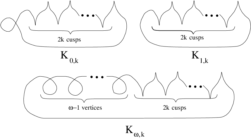
5. On the standard fronts $K_{\omega,k}$ (see Figure 5) $\operatorname{St}^{\prime}(L)$ , $J^{+}(L)$ , and $J^{-}(L)$ take the following values (independent of the choice of orientation and coorientation of the standard fronts):

(1)

\operatorname{St}^{\prime}(K_{0,k})=\frac{k}{2},\text{ }\operatorname{St}^{\prime}(K_{\omega+1,k})=\omega+\frac{k}{2}\text{ }(\omega=0,1,2,\dots);

(2)

J^{+}(K_{0,k})=-k,\text{ }J^{+}(K_{\omega+1,k})=-2\omega-k\text{ }(\omega=0,1,2,\dots);

(3)

J^{-}(K_{0,k})=-1,\text{ }J^{-}(K_{\omega+1,k})=-3\omega\text{ }(\omega=0,1,2,\dots);

where $k=0,1,2,\dots$ .

These values of the invariants on the standard fronts are chosen to make the invariants additive under a certain connected summation of fronts and independent of the choice of orientation and coorientation of the fronts.

3. Invariants of Fronts on Orientable Surfaces

3.1. Natural decomposition of the $K^{+}$ -stratum

3.1.1.

Let $B_{2}$ be a bouquet of two oriented circles and $b$ its base point. Let $L\in K^{+}$ be a front with a dangerous self-tangency point $q$ . It can be lifted to the mapping $\bar{L}:S^{1}\rightarrow STF$ that sends $p\in S^{1}$ to the point in $STF$ corresponding to the direction of the coorienting normal of $L$ at $L(p)$ . (Note that $q$ lifts to a double point $\bar{q}$ of $\bar{L}$ .)

Let $\alpha:S^{1}\rightarrow B_{2}$ be a continuous mapping such that:

a:: $\alpha(\bar{L}^{-1}(\bar{q}))=b$ ;
b:: $\alpha$ is injective on the complement of $\bar{L}^{-1}(\bar{q})$ ;
c:: The orientation of $B_{2}\setminus b$ induced by $\alpha$ coincides with the orientation of the circles of $B_{2}$ .

The mapping $\phi:B_{2}\rightarrow STF$ such that $\bar{L}=\phi\circ\alpha$ is called an associated with $L$ mapping of $B_{2}$ . (Note that the free homotopy class of a mapping of $B_{2}$ to $STF$ realized by $\phi$ is well defined modulo the orientation-preserving automorphism of $B_{2}$ interchanging the circles.)

Definition 3.1.2 (of $K^{+}$ -equivalence).

We say that $L_{1}\in K^{+}$ and $L_{2}\in K^{+}$ are $K^{+}$ -equivalent if there exist mappings of $B_{2}$ associated with the two of them that are free homotopic. This equivalence relation induces a decomposition of the $K^{+}$ -stratum into parts corresponding to different $K^{+}$ -equivalence classes. We denote by $[L^{+}]$ the $K^{+}$ -equivalence class corresponding to $L\in K^{+}$ and by $\mathcal{K}^{+}$ the set of all $K^{+}$ -equivalence classes.

3.2. Axiomatic description of $\overline{J^{+}}$

A natural way to introduce $J^{+}$ -type invariant of generic wave fronts on a surface $F$ is to take a function $\psi:\mathcal{K}^{+}\rightarrow{\mathbb{Z}}$ and to try to construct an invariant of generic fronts from a fixed connected component $\mathcal{C}$ of the space $\mathcal{L}$ (of all fronts on $F$ ) such that:

1. It increases by $\psi([L^{+}])$ under the positive crossing of the part of the $K^{+}$ -stratum that corresponds to a $K^{+}$ -equivalence class $[L^{+}]$ .

2. It does not change under crossings of $K^{-}$ -, $T$ -, $\Pi$ -, and $\Lambda$ -strata of the discriminant.

If for a given function $\psi:\mathcal{K}^{+}\rightarrow{\mathbb{Z}}$ there exists such an invariant of wave fronts from $\mathcal{C}$ , then we say that there exists a $\overline{J^{+}}$ invariant of fronts from $\mathcal{C}$ that integrates $\psi$ . Such $\psi$ is said to be $\overline{J^{+}}$ -integrable in $\mathcal{C}$ .

Theorem 3.2.1.

Let $F$ be an orientable surface, $\mathcal{C}$ a connected component of $\mathcal{L}$ , and $\psi:\mathcal{K}^{+}\rightarrow{\mathbb{Z}}$ a function. Then there exists a unique (up to an additive constant) invariant $\overline{J^{+}}$ of generic fronts from $\mathcal{C}$ which integrates $\psi$ .

The Proof of this Theorem (see Section 9) is based on Theorem 4.2.1.

Thus for orientable $F$ every $\psi:\mathcal{K}^{+}\rightarrow{\mathbb{Z}}$ is integrable in all connected components of $\mathcal{L}$ . However if $F$ is nonorientable, then such an invariant exists not for all functions $\psi$ . In Theorem 4.2.1 we present a condition on $\psi$ which is necessary and sufficient for it to be $\overline{J^{+}}$ -integrable in a fixed connected component of $\mathcal{L}$ .

Remark 3.2.2.

Most likely the proof of Theorem 3.2.1 in the case of $l\neq 1\in\pi_{1}(STF)$ can be obtained as a consequence of a version of E. Kalfagianni’s [12] Theorem $3.7$ for framed knots (if one formulates and proves this version). Similar remark holds for the $\overline{J^{-}}$ invariant of fronts on orientable surfaces, see Theorem 3.4.1, and for the part of statement I of Theorem 4.2.1 which is related to $\overline{J^{\pm}}$ invariants. Other statements of Theorem 4.2.1 about $\overline{J^{\pm}}$ invariants can not be obtained in this way. Statements of Theorems 3.6.1 and 4.2.1 about the existence of $\overline{\operatorname{St}^{\prime}}$ invariants also can not be obtained in this way.

3.2.3.

Connection with the standard $J^{+}$ -invariant. Since $\pi_{1}(ST{\mathbb{R}}^{2})={\mathbb{Z}}$ , there are countably many $K^{+}$ -equivalence classes of nongeneric planar fronts of fixed Whitney and Maslov indices. (The Whitney and Maslov indices of a planar front $L$ define the connected component of the space of planar fronts containing $L$ .) Thus the construction of $\overline{J^{+}}$ gives rise to a splitting of the standard $J^{+}$ invariant of V. Arnold. This is the splitting introduced by V. Arnold [5] in the case of planar fronts of the zero Whitney index and generalized to the case of arbitrary planar fronts by F. Aicardi [2].

3.3. Natural decomposition of the $K^{-}$ -stratum

3.3.1.

Let $B_{2}$ be a bouquet of two oriented circles and $b$ its base point. Let $L\in K^{-}$ be a front with a safe self-tangency point $q$ . It can be lifted to the mapping $\bar{L}$ from the oriented circle to $PTF$ (the projectivized tangent bundle of F) which sends $p\in S^{1}$ to the point in $PTF$ corresponding to the line normal to $L$ at $L(p)$ . (Note that $q$ lifts to a double point $\bar{q}$ of $\bar{L}$ .)

Let $\alpha:S^{1}\rightarrow B_{2}$ be a continuous mapping such that:

a:: $\alpha(\bar{L}^{-1}(\bar{q}))=b$ ;
b:: $\alpha$ is injective on the complement of $\bar{L}^{-1}(\bar{q})$ ;
c:: The orientation of $B_{2}\setminus b$ induced by $\alpha$ coincides with the orientation of the circles of $B_{2}$ .

The mapping $\phi:B_{2}\rightarrow PTF$ such that $\bar{L}=\phi\circ\alpha$ is called an associated with $L$ mapping of $B_{2}$ . (Note that the free homotopy class of a mapping of $B_{2}$ to $PTF$ realized by $\phi$ is well defined modulo the orientation-preserving automorphism of $B_{2}$ interchanging the circles.)

Definition 3.3.2 (of $K^{-}$ -equivalence).

We say that $L_{1}\in K^{-}$ and $L_{2}\in K^{-}$ are $K^{-}$ -equivalent if there exist associated with the two of them mappings of $B_{2}$ that are free homotopic. The $K^{-}$ -stratum is naturally decomposed into parts corresponding to different $K^{-}$ -equivalence classes. We denote by $[L^{-}]$ the $K^{-}$ -equivalence class corresponding to $L\in K^{-}$ and by $\mathcal{K}^{-}$ the set of all $K^{-}$ -equivalence classes.

3.4. Axiomatic description of $\overline{J^{-}}$

A natural way to introduce $J^{-}$ -type invariant of generic fronts on a surface $F$ is to take a function $\psi:\mathcal{K}^{-}\rightarrow{\mathbb{Z}}$ and to try to construct an invariant of generic wave fronts from a fixed connected component $\mathcal{C}$ of $\mathcal{L}$ such that:

1. It increases by $\psi([L^{-}])$ under a positive crossing of the part of the $K^{-}$ - stratum corresponding to a $K^{-}$ -equivalence class $[L^{-}]$ .

2. It does not change under crossings of $K^{+}$ -, $T$ -, $\Lambda$ -, and $\Pi$ -strata of the discriminant.

If for a given function $\psi:\mathcal{K}^{-}\rightarrow{\mathbb{Z}}$ there exists such an invariant of wave fronts from $\mathcal{C}$ , then we say that there exists a $\overline{J^{-}}$ invariant of fronts in $\mathcal{C}$ which integrates $\psi$ . Such $\psi$ is said to be $\overline{J^{-}}$ -integrable in $\mathcal{C}$ .

Theorem 3.4.1.

Let $F$ be an orientable surface, $\mathcal{C}$ a connected component of $\mathcal{L}$ , and $\psi:\mathcal{K}^{-}\rightarrow{\mathbb{Z}}$ a function. Then there exists a unique (up to an additive constant) invariant $\overline{J^{-}}$ of generic fronts from $\mathcal{C}$ which integrates $\psi$ .

The Proof of this Theorem is analogous to the Proof of Theorem 3.2.1 (see Section 9) and is based on Theorem 4.2.1 (see also 3.2.2).

Thus for orientable $F$ every $\psi:\mathcal{K}^{-}\rightarrow{\mathbb{Z}}$ is integrable in all connected components of $\mathcal{L}$ . However, if $F$ is nonorientable, then such an invariant exists not for all functions $\psi$ . In Theorem 4.2.1 we present a condition on $\psi$ which is necessary and sufficient for it to be $\overline{J^{-}}$ -integrable in a fixed connected component of $\mathcal{L}$ .

3.4.2.

Connection with the standard $J^{-}$ -invariant. Since $\pi_{1}(PT{\mathbb{R}}^{2})={\mathbb{Z}}$ , there are countably many $K^{-}$ -equivalence classes of nongeneric wave fronts on ${\mathbb{R}}^{2}$ of the fixed Whitney and Maslov indices. (Whitney and Maslov indices of a planar front $L$ define the connected component of the space of planar fronts containing $L$ .) Thus the construction of $\overline{J^{-}}$ gives rise to a splitting of the standard $J^{-}$ invariant of V. Arnold. This splitting is analogous to the splitting of $J^{+}$ introduced by V. Arnold [5] in the case of planar fronts of the zero Whitney index and generalized to the case of arbitrary planar wave fronts by F. Aicardi [2].

3.5. Natural decomposition of $T$ - and $\Pi$ -strata

3.5.1.

Let $B_{3}$ be a bouquet of three oriented circles with a fixed cyclic order on the set of them, and let $b$ be the base point of $B_{3}$ . Let $L\in T$ be a front on $F$ with a triple point $q$ .

Let $\alpha:S^{1}\rightarrow B_{3}$ be a continuous mapping such that:

a) $\alpha(L^{-1}(q))=b$ ;

b) $\alpha$ is injective on the complement of $L^{-1}(q)$ ;

c) The orientation induced by $\alpha$ on $B_{3}\setminus b$ coincides with the orientation of the circles of $B_{3}$ ;

d) The cyclic order induced on the set of circles of $B_{3}$ by traversing $\alpha(S^{1})$ according to the orientation of $S^{1}$ coincides with the fixed one.

The mapping $\phi:B_{3}\rightarrow F$ such that $L=\phi\circ\alpha$ is called an associated with $L$ mapping of $B_{3}$ . (Note that the free homotopy class of the mapping of $B_{3}$ to $F$ realized by $\phi$ is well defined modulo an automorphism of $B_{3}$ that preserves the orientation and the cyclic order of the circles.)

Definition 3.5.2 (of $T$ -equivalence).

We say that $L_{1}\in T$ and $L_{2}\in T$ are $T$ -equivalent if there exist associated with them mappings of $B_{3}$ which are free homotopic. The $T$ -stratum is naturally decomposed into parts corresponding to different $T$ -equivalence classes. Amazingly enough, the $T$ -equivalence relation induces also a subdivision of the $\Pi$ -stratum of the discriminant. To see it, one substitutes the cusp on $L\in\Pi$ by a small figure eight shape with a cusp on it (see Figure 4). As a result of this operation $L\in\Pi$ changes to a front $L^{\prime}\in T$ . (Note that $L$ and $L^{\prime}$ belong to the same component of $\mathcal{L}$ .) We take the $T$ -equivalence class of the front $L$ to be the $T$ -equivalence class of the front $L^{\prime}$ . We denote by $[L]$ the $T$ -equivalence class corresponding to $L\in T$ or to $L\in\Pi$ and by $\mathcal{T}$ the set of all $T$ -equivalence classes.

3.6. Axiomatic description of $\overline{\operatorname{St}^{\prime}}$

A natural way to introduce $\operatorname{St}^{\prime}$ -type invariants of generic wave fronts on $F$ is to take $\psi:\mathcal{T}\rightarrow{\mathbb{Z}}$ and to try to construct an invariant of generic wave fronts from a fixed connected component $\mathcal{C}$ of the space $\mathcal{L}$ (of all fronts on $F$ ) such that:

1. It does not change under crossings of $K^{\pm}$ - and $\Lambda$ - strata.

2. It increases by $\psi([L])$ under a positive crossing of the part of the $T$ -stratum that corresponds to a $T$ -equivalence class $[L]$ .

3. It increases by $\frac{1}{2}\psi([L])$ under a positive crossing of the part of the $\Pi$ -stratum that corresponds to a $T$ -equivalence class $[L]$ . (As it is explained in 8.1.3, one can not substitute $\frac{1}{2}$ by another constant and construct an invariant of this sort, unless $\psi$ is put to be identically zero on all $T$ -equivalence classes appearing on the $\Pi$ -stratum.)

If for a given function $\psi:\mathcal{T}\rightarrow{\mathbb{Z}}$ there exists such an invariant of wave fronts from $\mathcal{C}$ , then we say that there exists a $\overline{\operatorname{St}^{\prime}}$ invariant of fronts from $\mathcal{C}$ which integrates $\psi$ . Such $\psi$ is said to be $\overline{\operatorname{St}^{\prime}}$ -integrable in $\mathcal{C}$ .

Not all functions $\psi$ are integrable. In Theorem 4.2.1 we present a condition on $\psi$ which is necessary and sufficient for it to be integrable. In the case of orientable $F$ there is a simple condition which is sufficient for the integrability of $\psi$ .

Theorem 3.6.1.

Let $F$ be an orientable surface, $\mathcal{C}$ a connected component of $\mathcal{L}$ , and $\psi:\mathcal{T}\rightarrow{\mathbb{Z}}$ a function taking equal values on any two $T$ -equivalence classes such that:

a) The free homotopy classes of the mappings of $B_{3}$ representing them are different by an orientation-preserving automorphism of $B_{3}$ which changes the cyclic order of the circles.

b) The restrictions of the mappings representing these classes to one of the circles of $B_{3}$ are homotopic to a trivial loop.

Then there exists a unique (up to an additive constant) invariant $\overline{\operatorname{St}^{\prime}}$ of generic wave fronts from $\mathcal{C}$ which integrates $\psi$ .

The Proof of this Theorem is analogous to the Proof of Theorem 3.2.1 (see Section 9) and is based on Theorem 4.2.1 (cf. 3.2.2).

Note, that if $F$ is orientable, then a function $\psi:\mathcal{T}\rightarrow{\mathbb{Z}}$ described in Theorem 3.6.1 is integrable in all connected components of $\mathcal{L}$ .

In Section 4.2.1 we present a condition on $\psi$ which is necessary and sufficient for it to be $\overline{\operatorname{St}^{\prime}}$ -integrable in a fixed connected component of $\mathcal{L}$ .

3.6.2.

Connection with the standard $\operatorname{St}^{\prime}$ -invariant. Since ${\mathbb{R}}^{2}$ is simply connected, there is just one $T$ -equivalence class of nongeneric wave fronts on ${\mathbb{R}}^{2}$ . Thus the construction of $\overline{\operatorname{St}^{\prime}}$ does not give anything new in the classical case of planar wave fronts.

4. Necessary and sufficient conditions for the integrability of functions

4.1. Obstructions for the integrability

Let $\psi:\mathcal{T}\rightarrow{\mathbb{Z}}$ be a function, and let $\gamma$ be a generic loop in a connected component $\mathcal{C}$ of $\mathcal{L}$ . Let $I_{1}$ and $I_{2}$ be the sets of moments when $\gamma$ crosses respectively $T$ - and $\Pi$ -strata. Let $\{\sigma_{i}\}_{i\in I_{1}}$ and $\{\sigma_{i}\}_{i\in I_{2}}$ be the signs of the corresponding crossings of the strata, and let $\{s_{i}\}_{i\in I_{1}}$ and $\{s_{i}\}_{i\in I_{2}}$ be the $T$ -equivalence classes corresponding to the parts of the strata where the crossings occurred. We call

(4)

\Delta_{\overline{\operatorname{St}^{\prime}}}(\gamma)=\sum_{i\in I_{1}}\sigma_{i}\psi(s_{i})+\sum_{i\in I_{2}}\sigma_{i}\frac{1}{2}\psi(s_{i})

the change of $\overline{\operatorname{St}^{\prime}}$ along $\gamma$ . If $\Delta_{\overline{\operatorname{St}^{\prime}}}(\gamma)=0$ , then $\psi$ is said to be integrable along $\gamma$ . In a similar way we introduce the notion of integrability along $\gamma$ for integer valued functions on $\mathcal{K}^{+}$ and on $\mathcal{K}^{-}$ . (For this purpose we use the intersections of $\gamma$ with $K^{+}$ - and $K^{-}$ -strata respectively.) The changes of $\overline{J^{-}}$ and of $\overline{J^{+}}$ along $\gamma$ are also defined in a similar way. (Using Lemma 8.0.1 and the versions of it for the $\overline{J^{\pm}}$ invariants one can verify that the change along $\gamma$ depends only on the homology class realized by $\gamma$ in $H_{1}(\mathcal{L},{\mathbb{Z}})$ .)

Clearly if a function $\psi$ is integrable in $\mathcal{C}$ , then it is integrable along any generic loop $\gamma\subset\mathcal{C}$ . In this section we describe two loops $\gamma_{1}$ and $\gamma_{2}$ in $\mathcal{C}$ such that integrability along them implies integrability in $\mathcal{C}$ . In a sense, the changes along them are the only obstructions for the integrability. The loop $\gamma_{1}$ is going to be well defined (and needed) only in the case of $\mathcal{C}$ consisting of orientation-preserving fronts on $F$ . The loop $\gamma_{2}$ is going to be well defined (and needed) only in the case of $F$ being a Klein bottle and $\mathcal{C}$ consisting of orientation-preserving fronts on it.

4.1.1.

Loop $\gamma_{1}$ . Let $\mathcal{C}$ be a connected component of $\mathcal{L}$ consisting of orientation-preserving fronts, and let $L\in\mathcal{C}$ be a generic front. Let $\gamma_{1}$ be the loop starting at $L$ which is described below.

Deform $L$ along a generic path $t$ in $\mathcal{C}$ to get two opposite kinks, as it shown in Figure 6. Make the first kink small and slide it along the front till it comes back. We require the deformation to be such that at each moment of time points of $L$ located outside of a small neighborhood of the kink do not move. (In Figure 7 and Figure 8 it is shown how the kink passes through a neighborhood of a double and of a cusp point.) Finally deform $L$ to its original shape along $t^{-1}$ .

4.1.2.

Loop $\gamma_{2}$ . Let $L$ be a generic orientation-preserving front on the Klein bottle $K$ . Let $\gamma_{2}\subset\mathcal{C}$ be the loop starting at $L$ that is constructed below.

Consider $K$ as a quotient of a rectangle modulo the identification on its sides shown in Figure 9. Let $p$ be the orientation covering $T^{2}\rightarrow K$ . There is a loop $\alpha$ in the space of all autodiffeomorphisms of $T^{2}$ which is the sliding of $T^{2}$ along the unit vector field parallel to the lifting of the curve $c\subset K$ (see Figure 9). Since $L$ is an orientation-preserving front it can be lifted to a front $L^{\prime}$ on $T^{2}$ . The loop $\gamma_{2}$ is the composition of $p$ and of the sliding of $L^{\prime}$ induced by $\alpha$ .

4.2. Main Integrability Theorem

Now we are ready to formulate the main integrability theorem.

Theorem 4.2.1.

Let $F$ be a surface (not necessarily compact or orientable), $\mathcal{C}$ a connected component of $\mathcal{L}$ , and $L\in\mathcal{C}$ a generic front. Let $\psi_{1}:\mathcal{T}\rightarrow{\mathbb{Z}}$ , $\psi_{2}:\mathcal{K}^{+}\rightarrow{\mathbb{Z}}$ and $\psi_{3}:\mathcal{K}^{-}\rightarrow{\mathbb{Z}}$ be functions.

I:: If $\mathcal{C}$ consists of orientation-reversing fronts on $F$ , then there exists a $\overline{\operatorname{St}^{\prime}}$ (resp. $\overline{J^{+}}$ , resp. $\overline{J^{-}}$ ) invariant which integrates $\psi_{1}$ (resp. $\psi_{2}$ , resp. $\psi_{3}$ ) in $\mathcal{C}$ .
II:: If $\mathcal{C}$ consists of orientation-preserving fronts and $F\neq K$ , then the condition that $\psi_{1}$ (resp. $\psi_{2}$ , resp. $\psi_{3}$ ) is integrable along the loop $\gamma_{1}$ starting at $L$ is necessary and sufficient for the existence of a $\overline{\operatorname{St}^{\prime}}$ (resp. $\overline{J^{+}}$ , resp. $\overline{J^{-}}$ ) invariant which integrates $\psi_{1}$ (resp. $\psi_{2}$ , resp. $\psi_{3}$ ) in $\mathcal{C}$ .
III:: If $\mathcal{C}$ consists of orientation-preserving fronts and $F=K$ , then the condition that $\psi_{1}$ (resp. $\psi_{2}$ , resp. $\psi_{3}$ ) is integrable along loops $\gamma_{1}$ and $\gamma_{2}$ starting at $L$ is necessary and sufficient for the existence of a $\overline{\operatorname{St}^{\prime}}$ (resp. $\overline{J^{+}}$ , resp. $\overline{J^{-}}$ ) invariant which integrates $\psi_{1}$ (resp. $\psi_{2}$ , resp. $\psi_{3}$ ) in $\mathcal{C}$ .

For the proof of Theorem 4.2.1 see Section 8 (cf. also 3.2.2).

4.2.2.

Remarks to Theorem 4.2.1. If an invariant from the statement of the Theorem exists, then it is unique up to an additive constant.

The choice of $L\in\mathcal{C}$ does not matter and to check integrability of a given function it is easier to take $L\in\mathcal{C}$ that already has a small kink. Clearly all the crossings of the discriminant under the deformation $\gamma_{1}$ of $L$ occur when the kink passes through a neighborhood of a double point or of a cusp of $L$ . It easy to verify that inputs into $\Delta(\gamma_{1})$ of the crossings of the discriminant corresponding to the kink passing through a neighborhood of a cusp occur in pairs and cancel out. A kink passes through a neighborhood of a double point $x$ twice (once along each of the two intersecting branches). One can verify that if $x$ separates the front into two orientation-preserving loops, then the inputs into $\Delta_{\overline{J^{\pm}}}(\gamma_{1})$ corresponding to $x$ also cancel out.

A straightforward modification of the proof of Theorem 4.2.1 shows that it holds for $\psi_{1}$ , $\psi_{2}$ , and $\psi_{3}$ taking values in any torsion free Abelian group.

4.3. A very general integrability Theorem

From the proof of Theorem 4.2.1 one can see that for any $\alpha\in H_{1}({\mathcal{C}},{\mathbb{Z}})$ a certain (nonzero) multiple of $\alpha$ is equal to a sum of a homology class realizable by a loop not crossing the discriminant and of a linear combination of homology classes realized by $\gamma_{i}$ , $i\in\{1,2,3\}$ (see 8.2.12 for the definition of $\gamma_{3}$ ). (If $\gamma_{i}$ for some $i\in\{1,2,3\}$ is not defined in $\mathcal{C}$ , then it does not participate in the linear combination.) A very important consequence of this is the following very general statement.

Let $\Sigma$ be the discriminant in $\mathcal{C}$ , $G$ an Abelian group, and $\chi$ a $G$ -valued invariant of generic fronts in $\mathcal{C}$ , that is a mapping from the set of the connected components of ${\mathcal{C}}\setminus\Sigma$ to $G$ . (The condition that $\chi$ takes values in an Abelian group is not very restrictive, since $\chi$ with values in an abstract set $S$ can be viewed as an invariant taking values in ${\mathbb{Z}}[S]$ an Abelian group of abstract finite integer linear combinations of the elements of $S$ .)

The invariant $\chi$ gives rise to the invariant $\chi^{\prime}$ of nongeneric fronts with one singular point (which is singular of codimension one), that is a mapping to $G$ from the set of connected components of $\Lambda$ -, $K^{\pm}$ -, $\Pi$ -, and $T$ -strata. The value of $\chi^{\prime}$ on a component of a stratum is set to be the difference between the values of $\chi$ on the positive and negative sides of it. (The positive side of the $\Lambda$ -stratum is the one with more cusps.) In an obvious sense $\chi^{\prime}$ is a derivative of $\chi$ .

A very natural question is the following (cf. Kalfagianni [12]): does a given $G$ -valued function $\chi^{\prime}$ on the set of connected components of $\Lambda$ -, $K^{\pm}$ -, $\Pi$ -, and $T$ -strata correspond to some $\chi$ under the construction above? (Is the integral of $\chi^{\prime}$ well defined?)

For a generic loop $\gamma$ in $\mathcal{C}$ put $\Delta_{\chi}(\gamma)=\sum_{x\in\gamma\cap\Sigma}\operatorname{sign}(x)\chi^{\prime}(x)$ . Clearly the necessary condition for the existence of $\chi$ is that $\Delta_{\chi}(\gamma)=0$ for any small generic loop $\gamma$ going around a codimension two stratum of $\mathcal{C}$ (see 8.1.1 for the list of the strata). We call this condition a local integrability condition. If the local integrability condition is satisfied, then the change of $\Delta_{\chi}(\gamma)$ depends only on the homology class of the generic loop $\gamma$ . Using the observation above one can easily modify the proof of Theorem 4.2.1 to get the following very general Theorem.

Theorem 4.3.1.

Let $G$ be a torsion free Abelian group, $\mathcal{C}$ a connected component of $\mathcal{L}$ , and $\chi^{\prime}$ a $G$ -valued invariant of nongeneric fronts from $\mathcal{C}$ whose only nongeneric singularity is one codimension one singular point. Then $\chi^{\prime}$ is a derivative of an invariant $\chi$ of generic fronts from $\mathcal{C}$ if and and only if $\chi^{\prime}$ satisfies the local integrability condition and $\Delta_{\chi}(\gamma_{i})=0$ for those $i\in\{1,2,3\}$ for which $\gamma_{i}$ is well defined in $\mathcal{C}$ .

Potential interesting application of this Theorem lie in the theory of Legendrian knots in $ST^{*}F$ . The invariants of Legendrian knots correspond to $\chi^{\prime}$ being identically zero on all the components of $\Lambda$ -, $K^{-}$ -, $\Pi$ -, and $T$ -strata. In this case the local integrability condition appears to be very simple. Using this Theorem one can easily obtain the generalizations of other local invariants of planar fronts studied by F. Aicardi [1].

5. Singularity theory interpretation of the invariants

The invariants $\overline{\operatorname{St}^{\prime}}$ , $\overline{J^{+}}$ , and $\overline{J^{-}}$ admit a rather simple singularity theory interpretation. Namely, the set of all $K^{+}$ -equivalence classes appearing on the discriminant in $\mathcal{C}$ enumerates the components of the normalized dangerous self-tangency part of the discriminant in $\mathcal{C}$ . If $F$ is orientable then similar facts are true for the sets of $K^{-}$ - and $T$ -equivalence classes. (See Proposition 5.2.6.)

In this section we introduce finer versions of equivalence relations to obtain the complete classification of the components of the four parts of the discriminant arising under the normalizations described below. (This is done for all $F$ , not necessarily orientable, see Theorem 5.2.5.) We also formulate the corresponding versions of Theorem 4.2.1

5.1. Normalizations

Let $S^{1}(2)$ be the configuration space of unordered pairs of distinct points on $S^{1}$ . Let $\mathcal{N}^{+}$ be the subspace of $S^{1}(2)\times\mathcal{L}$ consisting of $t\times L\in S^{1}(2)\times\mathcal{L}$ such that $L$ maps the two points from $t$ to one point in $F$ and the coorienting normals of $L$ at these two points have the same direction. (This is a normalization of the part of the discriminant containing points of dangerous self-tangency.)

We say that $n_{1}^{+},n_{2}^{+}\in\mathcal{N}^{+}$ are $\overline{K^{+}}$ -equivalent if they belong to the same path connected component of $\mathcal{N}^{+}$ . Clearly for $L\in K^{+}$ there is a unique $\overline{K^{+}}$ -equivalence class associated with it. Thus the $\overline{K^{+}}$ -equivalence relation induces a decomposition of the $K^{+}$ -stratum.

Similarly we normalize the part of the discriminant containing safe self-tangency (resp. triple) points and introduce the notion of $\overline{K^{-}}$ - (resp. $\overline{T}$ -) equivalence relation of fronts in $K^{-}$ (resp. in $T$ ).

We consider the following normalization of the closure of the $\Pi$ -stratum. Let $N$ be the closure of the subspace of $S^{1}\times S^{1}\times\mathcal{L}$ consisting of $t_{1}\times t_{2}\times L$ such that $t_{1}\neq t_{2}$ , $L$ has a cusp point at $t_{1}$ , and $L(t_{1})=L(t_{2})$ . We say that $n_{1},n_{2}\in\mathcal{N}$ are $\overline{\Pi}$ -equivalent if they belong to the same path connected component of $\mathcal{N}$ . Clearly, for $L\in\Pi$ there is a unique $\overline{\Pi}$ -equivalence class associated with it. Thus the $\overline{\Pi}$ -equivalence relation induces a decomposition of the $\Pi$ -stratum. We denote by $\overline{\mathcal{P}}$ the set of all $\overline{\Pi}$ -equivalence classes.

Remark 5.1.1.

The reason why we treat cusp crossings differently from other codimension one singularities is that in the neighborhood of two of the codimension two strata of the discriminant the $\Pi$ -stratum is not connected. (These strata are $\Lambda\Lambda$ and $\Pi\Lambda$ in the notation of Theorem 8.1.1, see Figure 13.) One can verify that the two branches on the bifurcation diagrams of these singularities corresponding to the $\Pi$ -stratum belong to the same irreducible real algebraic curve, and hence it is natural to glue together the components of the $\Pi$ -stratum around these codimension two strata.

5.2. Description of the sets of $\overline{K^{+}}$ -, $\overline{K^{-}}$ -, $\overline{T}$ -, and $\overline{\Pi}$ -equivalent fronts

In this subsection we state Theorem 5.2.5 which gives an explicit description of the sets of components of the four parts of the discriminant arising under the normalizations described above. These components are enumerated by the sets of $K^{+}_{i}$ -, $K^{-}_{i}$ -, $T_{i}$ -, and $\Pi_{i}$ -equivalence classes introduced below.

We fix $d\in STF$ and denote by $\pi_{1}(STF)$ and $\pi_{1}(PTF)$ the groups $\pi_{1}(STF,d)$ and $\pi_{1}(PTF,p(d))$ . (Here $p:STF\rightarrow PTF$ is the natural double covering.) The definitions introduced below are similar to the ones introduced by Inshakov [10] in the case of immersed curves on a surface. For this reason we use a subscript $i$ in the notation of the arising equivalence classes.

Definition 5.2.1 (of $K_{i}^{+}$ -equivalence).

Let $R_{K^{+}}$ be the set consisting of all triples $(\delta_{1},\delta_{2},i)\in\pi_{1}(STF)\oplus\pi_{1}(STF)\oplus{\mathbb{Z}}$ such that $i$ is even provided that $\operatorname{pr}^{2}(\delta_{1}\delta_{2})$ is an orientation-preserving loop in $F$ and odd otherwise.

The Legendrian curve $l$ corresponding to $L\in K^{+}$ has a double point separating it into two oriented loops. Deform $l$ preserving the double point so that the double point is located at $d$ . Choosing one of the two loops of $l$ we obtain an ordered set of two elements $\delta_{1},\delta_{2}\in\pi_{1}(STF)$ . We also correspond to the front its Maslov index $\mu(L)\in{\mathbb{Z}}$ that is even if and only if $l=\delta_{1}\delta_{2}$ projects to an orientation-preserving loop in $F$ . Thus we obtain an element of $R_{K^{+}}$ corresponding to the deformed $l$ . There is a unique $K_{i}^{+}$ -equivalence class of elements of $R_{K^{+}}$ corresponding to the undeformed $l$ , where two elements of $R_{K^{+}}$ are $K_{i}^{+}$ -equivalent if one can be transformed to the other by the consequent actions of the following groups (which all act trivially on the last summand in $R_{K^{+}}$ ):

1. $\pi_{1}(STF)$ whose elements act via conjugation of the first two summands in $R_{K^{+}}$ . (This corresponds to the ambiguity in deforming $l$ , so that the double point is located at $d$ .)

2. ${\mathbb{Z}}_{2}$ which acts via the cyclic permutation of the first two summands. (This corresponds to the ambiguity in the choice of one of the two loops of $l$ .)

The set of all $K_{i}^{+}$ -equivalence classes of elements of $R_{K^{+}}$ is denoted by $\mathcal{K}^{+}_{i}$ .

Definition 5.2.2 (of $K^{-}_{i}$ -equivalence).

Let $p:STF\rightarrow PTF$ be the natural covering, $\pi_{1}^{+}(PTF)=p_{*}(\pi_{1}(STF))$ , and let $\pi_{1}^{-}(PTF)$ be a set $\pi_{1}(PTF)\setminus\pi_{1}^{+}(PTF)$ . Let $R_{K^{-}}$ be the set of all $(\delta_{1},\delta_{2},i)\in\pi_{1}^{-}(PTF)\oplus\pi_{1}^{-}(PTF)\oplus{\mathbb{Z}}$ such that $i$ is even provided that $\operatorname{pr}^{2}(\delta_{1}\delta_{2})$ is an orientation-preserving loop in $F$ and odd otherwise.

Let $L\in K^{-}$ be a front and $a\in S^{1}$ one of the two points projecting to the self-tangency point. Deform $l$ keeping the two preimages of the tangency point opposite to each other in the fiber of $STF$ , so that $l(a)$ is located at $d\in STF$ . The point $p(d)$ separates $p(l)$ into two closed loops. Thus we obtain an ordered set of two elements $\delta_{1},\delta_{2}\in\pi_{1}(PTF)$ corresponding to the deformed $l$ . (The first element is the projection of the arc of $l$ that has $a$ as its starting point.) Clearly both elements belong to $\pi_{1}^{-}(PTF)$ . We also correspond to the front its Maslov index $\mu(L)$ , which is even if and only if $l=\delta_{1}\delta_{2}$ projects to an orientation-preserving loop in $F$ . Thus we obtain an element of $R_{K^{-}}$ corresponding to the deformed $l$ .

There is a unique $K_{i}^{-}$ -equivalence class of elements of $R_{K^{-}}$ corresponding to the undeformed $l$ , where two elements of $R_{K^{-}}$ are $K_{i}^{-}$ -equivalent if one can be transformed to the other by an action of the following group (which acts trivially on the last summand in $R_{K^{-}}$ ):

The group is the index two subgroup of $\pi_{1}(PTF)\oplus{\mathbb{Z}}_{2}$ which is $\bigl(\pi_{1}^{+}(PTF)\oplus 0\bigr)\cup\bigl(\pi_{1}^{-}(PTF)\oplus 1\bigr)$ . The action of the first summand of the group is via conjugation of the first two summands in $R_{K^{-}}$ and the action of the second summand of the group is via permutation of the first two summands in $R_{K^{-}}$ . (The factorization by the action of this group corresponds to the ambiguity in the choices of one of the two points of $S^{1}$ that project to the selftangency point and in the deformation of $l$ so that the chosen point is located at $d\in STF$ .)

The set of all $K_{i}^{-}$ -equivalence classes of elements of $R_{K^{-}}$ is denoted by $\mathcal{K}^{-}_{i}$ .

Definition 5.2.3 (of $T_{i}$ -equivalence).

Let $R_{T}$ be the set consisting of all quadruples $(\delta_{1},\delta_{2},\delta_{3},i)\in\pi_{1}(STF)\oplus\pi_{1}(STF)\oplus\pi_{1}(STF)\oplus{\mathbb{Z}}$ such that $i$ is even provided that $\operatorname{pr}^{2}(\delta_{1}\delta_{2}\delta_{3})$ is an orientation-preserving loop in $F$ and odd otherwise.

Let $L\in T$ be a front. Deform the lifting $l$ of $L$ in the neighborhood of the fiber of $\operatorname{pr}^{2}$ over the triple point, so that it maps the three preimages of the triple point to one point in $STF$ . (This triple point in $STF$ separates $l$ into three cyclicly ordered oriented loops based at this point.) Then deform the singular knot $l$ (preserving the triple point), so that the triple point is located at $d\in STF$ . Choosing which one of the three closed arcs of $l$ is first we obtain an ordered set of three elements of $\pi_{1}(STF)$ . We also correspond to the front its Maslov index $\mu(L)\in{\mathbb{Z}}$ , which is even if and only if $l=\delta_{1}\delta_{2}\delta_{3}$ projects to an orientation preserving loop in $F$ . Thus we obtain an element of $R_{T}$ corresponding to the deformed $l$ . There is a unique $T_{i}$ -equivalence class of elements of $R_{T}$ corresponding to the undeformed $l$ , where two elements of $R_{T}$ are $T_{i}$ -equivalent if one of them can be transformed to the other by the consequent action of the following groups (which all act trivially on the last summand in $R_{T}$ ):

1. ${\mathbb{Z}}^{3}$ whose element $(i_{1},i_{2},i_{3})$ acts on $(\delta_{1},\delta_{2},\delta_{3},i)\in R_{T}$ by mapping it to $(f^{i_{1}}_{2}\delta_{1}f^{-i_{2}}_{2},f^{i_{2}}_{2}\delta_{2}f^{-i_{3}}_{2},f^{i_{3}}_{2}\delta_{3}f^{-i_{1}}_{2},i)$ . (This corresponds to the ambiguity in deforming $l$ to a singular knot with a triple point.)

2. $\pi_{1}(STF)$ whose elements act via conjugation of the first three summands. (This corresponds to the ambiguity in deforming a singular knot with a triple point, so that the triple point is at $d$ .)

3 ${\mathbb{Z}}_{3}$ which acts via the cyclic permutation of the first three summands. (This corresponds to the ambiguity in the choice of the first closed arc of $l$ .)

The set of all $T_{i}$ -equivalence classes of elements of $R_{T}$ is denoted by $\mathcal{T}_{i}$ .

Definition 5.2.4 (of $\Pi_{i}$ -equivalence).

Let $R_{\Pi}$ be the set consisting of all quadruples $(\delta_{1},\delta_{2},j,i)\in\pi_{1}(STF)\oplus\pi_{1}(STF)\oplus{\mathbb{Z}}_{2}\oplus{\mathbb{Z}}$ such that $i$ is even provided that $\operatorname{pr}^{2}(\delta_{1}\delta_{2})$ is an orientation-preserving loop in $F$ and odd otherwise.

Fix a local orientation at $\operatorname{pr}^{2}(d)\in F$ . Let $L\in\Pi$ be a front. The direction of rotation of the coorienting normal at the cusp point $x$ under traversing of a small neighborhood (in $L$ ) of it along the orientation of $L$ defines a local orientation at $x\in F$ . Deform the lifting $l$ of $L$ , so that $l$ maps the two preimages of the cusp crossing point to one point in $STF$ . The double point of $l$ separates it into two oriented loops $\delta_{1},\delta_{2}$ based at this point. The set of these two loops is ordered by taking the loop corresponding to the branch of the cusp going away from it as the first one. Deform $l$ in $STF$ (preserving the double point), so that the double point is located at $d\in STF$ . Transfer the local orientation at the original location of the cusp along the projection of the path of the double point of $l$ under the deformation to get the local orientation at $\operatorname{pr}^{2}(d)$ . It is an element of ${\mathbb{Z}}_{2}$ . We also correspond to $L$ its Maslov index $\mu(L)\in{\mathbb{Z}}$ . Clearly $\mu(L)$ is even if and only if $\operatorname{pr}^{2}(l)=\operatorname{pr}^{2}(\delta_{1}\delta_{2})$ is an orientation-preserving loop in $F$ .

Hence we obtain an element of $R_{\Pi}$ corresponding to the deformed $l$ . One verifies that there is a unique $\Pi_{i}$ -equivalence class of elements of $R_{\Pi}$ associated with the undeformed $l$ , where two elements of $R_{\Pi}$ are said to be $\Pi_{i}$ -equivalent if one of them can be transformed to the other by a consequent action of the following groups (which all act trivially on the last summand in $R_{\Pi}$ ):

1. ${\mathbb{Z}}^{2}$ whose element $(i_{1},i_{2})$ acts on $(\delta_{1},\delta_{2},j,i)\in R_{\Pi}$ by mapping it to $(f_{2}^{i_{1}}\delta_{1}f_{2}^{-i_{2}},$ $f_{2}^{i_{2}}\delta_{2}f_{2}^{-i_{1}},j,i)$ . (Factorization by this action corresponds to the ambiguity in deforming $l$ to a singular knot with a double point.)

2. $\pi_{1}(STF)$ whose element $\alpha$ acts on the first two summands by conjugation and acts trivially on the ${\mathbb{Z}}_{2}$ -summand if and only if $\operatorname{pr}^{2}(\alpha)$ is an orientation-preserving loop in $F$ . (Factorization by this action corresponds to the ambiguity in deforming a singular knot with a double point, so that the double point is located at $d$ .)

3. ${\mathbb{Z}}_{2}$ whose elements act nontrivially only if $\operatorname{pr}^{2}(\delta_{1})$ or $\operatorname{pr}^{2}(\delta_{2})$ is $1\in\pi_{1}(F)$ , in which case the action is by permutation of the first two summands. (The reason for this factorization is that we want to be able to identify the sets of $\Pi_{i}$ - and $\overline{\Pi}$ -equivalence classes, and one can verify that under the passage through a point of degree $5/4$ along the $\Pi$ -stratum the order of the two loops is changed, see Figure 13.)

The set of all $\Pi_{i}$ -equivalence classes of elements of $R_{\Pi}$ is denoted by $\mathcal{P}_{i}$ .

One verifies that:

1. if $L_{1},L_{2}\in K^{+}$ are $\overline{K^{+}}$ -equivalent, then they are $K^{+}_{i}$ -equivalent;

2. if $L_{1},L_{2}\in K^{-}$ are $\overline{K^{-}}$ -equivalent, then they are $K^{-}_{i}$ -equivalent;

3. if $L_{1},L_{2}\in T$ are $\overline{T}$ -equivalent, then they are $T_{i}$ -equivalent;

4. if $L_{1},L_{2}\in\Pi$ are $\overline{\Pi}$ -equivalent, then they are $\Pi_{i}$ -equivalent.

And we get mappings $\psi^{+}:\overline{\mathcal{K}^{+}}\rightarrow{\mathcal{K}^{+}_{i}}$ , $\psi^{-}:\overline{\mathcal{K}^{-}}\rightarrow{\mathcal{K}^{-}_{i}}$ , $\psi:\overline{\mathcal{T}}\rightarrow{\mathcal{T}_{i}}$ , $\psi^{\pi}:\overline{\mathcal{P}}\rightarrow{\mathcal{P}_{i}}$ .

Theorem 5.2.5.

The mappings $\psi^{+}$ , $\psi^{-}$ , $\psi$ , and $\psi^{\pi}$ are bijective.

For the proof of Theorem 5.2.5 see Section 10.

The connected components of the normalization of the dangerous self-tangency part of the discriminant in $\mathcal{C}$ are in a natural one-to-one correspondence with the set of $K^{+}$ -equivalence classes of fronts from $\mathcal{C}$ . Analogous statement is true for the safe self-tangency and triple point parts of the discriminant, provided that $F$ is orientable.

Let $\mathcal{C}$ be a connected component of $\mathcal{L}$ . Let $\overline{\mathcal{T}_{\mathcal{C}}}$ , $\overline{\mathcal{K}^{+}_{\mathcal{C}}}$ , $\overline{\mathcal{K}^{-}_{\mathcal{C}}}$ , $\mathcal{T}_{\mathcal{C}}$ , $\mathcal{K}^{+}_{\mathcal{C}}$ , and $\mathcal{K}^{-}_{\mathcal{C}}$ be the sets of equivalence classes corresponding to fronts from $\mathcal{C}$ . Similarly to the case above we get the mappings $\phi_{\mathcal{C}}:\overline{\mathcal{T}_{\mathcal{C}}}\rightarrow\mathcal{T}_{\mathcal{C}}$ , $\phi^{+}_{\mathcal{C}}:\overline{\mathcal{K}^{+}_{\mathcal{C}}}\rightarrow\mathcal{K}^{+}_{\mathcal{C}}$ , and $\phi^{-}_{\mathcal{C}}:\overline{\mathcal{K}^{-}_{\mathcal{C}}}\rightarrow\mathcal{K}^{-}_{\mathcal{C}}$ .

Proposition 5.2.6.

The mapping $\phi^{+}_{\mathcal{C}}$ is bijective. The mappings $\phi^{-}_{\mathcal{C}}$ and $\phi_{\mathcal{C}}$ are bijective provided that $F$ is orientable.

For the proof of Proposition 5.2.6 see Section 10.1.

One can construct examples showing that for nonorientable surfaces the mappings $\phi^{-}_{\mathcal{C}}$ and $\phi_{\mathcal{C}}$ fail to be injective.

5.3. An important generalization of Theorem 4.2.1

We say that an invariant of generic fronts is of $J^{+}$ -type if it changes under crossings of the $K^{+}$ -stratum and does not change under crossings of the other codimension one strata of the discriminant. Similarly to 4.3 for such an invariant with values in an Abelian group $G$ we define its $n$ -th derivative, which assigns an element of $G$ to a front whose only nongeneric singularities are $n$ points of dangerous order one self-tangency. The invariant is said to be of order $k$ if $k$ is the minimal number such that the $k+1$ -st derivative of the invariant is identically zero.

The invariants whose change under the crossing of a part of the $K^{+}$ -stratum depends only on the $\overline{K^{+}}$ -equivalence class corresponding to the part are exactly the $J^{+}$ -type invariants of order one. Proposition 5.2.6 implies that every such invariant of fronts from $\mathcal{C}$ can be obtained as a $\overline{J^{+}}$ invariant for some $\psi:\mathcal{K}^{+}\rightarrow{\mathbb{Z}}$ .

Such interpretation does not hold if we do not restrict ourselves to one component $\mathcal{C}$ of $\mathcal{L}$ and consider invariants defined in all components. The reason is that nongeneric fronts belonging to different components of $\mathcal{L}$ , and hence realizing different $\overline{K^{+}}$ -equivalence classes, can realize the same $K^{+}$ -equivalence class. (This happens only if the Maslov indices of the two fronts are different.) Theorem 5.2.5 says that there is a natural bijection between the sets $\mathcal{K}^{+}_{i}$ and $\overline{\mathcal{K}^{+}}$ . Hence every order one $J^{+}$ -type invariant of fronts on $F$ can be obtained by integration in all components of $\mathcal{L}$ of some $\psi:\mathcal{K}^{+}_{i}\rightarrow{\mathbb{Z}}$ . One can easily verify that statements of Theorem 4.2.1 hold if one substitutes $K^{+}$ - by $K^{+}_{i}$ -equivalence classes in the formulation of the Theorem and in the axiomatic description of the $\overline{J^{+}}$ invariant. (The proof of this version of the theorem is the same as the original one.)

The interpretation of the $\overline{J^{-}}$ invariant is similar to the one of $\overline{J^{+}}$ , with the difference that in the case of nonorientable $F$ not every order one $J^{-}$ -type invariant of fronts in $\mathcal{C}$ is an integral of some $\psi:\mathcal{K}^{-}\rightarrow{\mathbb{Z}}$ . (For nonorientable $F$ two fronts from $\mathcal{C}$ realizing the same $K^{-}$ -equivalence class can realize different $\overline{K^{-}}$ -classes.) Similarly to the case of $J^{+}$ , we see that every order one $J^{-}$ -type invariant of fronts in $\mathcal{L}$ can be obtained by integration in all components of $\mathcal{L}$ of some $\psi:\mathcal{K}^{-}_{i}\rightarrow{\mathbb{Z}}$ . One verifies that statements of Theorem 4.2.1 hold if one substitutes $K^{-}$ - by $K^{-}_{i}$ -equivalence classes in the formulation of the Theorem and in the axiomatic description of the $\overline{J^{-}}$ invariant.

The operation of changing $L\in\Pi$ to $L^{\prime}\in T$ shown in Figure 4 induces a decomposition of the $\Pi$ -stratum into parts corresponding to different $T_{i}$ -equivalence classes, and one obtains the corresponding version of Theorem 4.2.1.

One verifies that this operation induces a mapping $g:\mathcal{P}_{i}\rightarrow\mathcal{T}_{i}$ that sends a $\Pi_{i}$ -equivalence class of $(\delta_{1},\delta_{2},i,j)\in R_{\Pi}$ to a $T_{i}$ -equivalence class of $(\delta_{1},\delta_{2},1,j)\in R_{T}$ . (Here $1\in\pi_{1}(STF)$ is a class of a trivial loop.) One verifies that the part of the $\Pi$ -stratum corresponding to $\pi_{i}\in\mathcal{P}_{i}$ is adjacent (along the $\Pi\Lambda$ -stratum, see 8.1.1) to the part of the $T$ -stratum corresponding to $g(\pi_{i})\in\mathcal{T}_{i}$ . This means (see 8.1.3) that if the magnitudes of the change of a ${\operatorname{St}^{\prime}}$ -type invariant under the crossings of $T$ - and $\Pi$ -strata depend only on the component of the normalization corresponding to the crossings, then the change under the positive crossing of the $\pi_{i}$ -part of the $\Pi$ -stratum should be half of the change under the positive crossing of the $g(\pi_{i})$ -part of the $T$ -stratum. Every ${\operatorname{St}^{\prime}}$ -type invariant of this sort is a $\overline{\operatorname{St}^{\prime}}$ invariant for some $\psi:\mathcal{T}_{i}\rightarrow{\mathbb{Z}}$ .

An important observation is that Remarks 4.2.2 hold for the versions of the three invariants described above.

Remark 5.3.1.

A front with a dangerous self-tangency point lifts to a singular Legendrian knot in $ST^{*}F$ . (It has a double point.) One can verify that order one $J^{+}$ -type invariants of fronts are exactly order one invariants of Legendrian knots in $ST^{*}F$ .

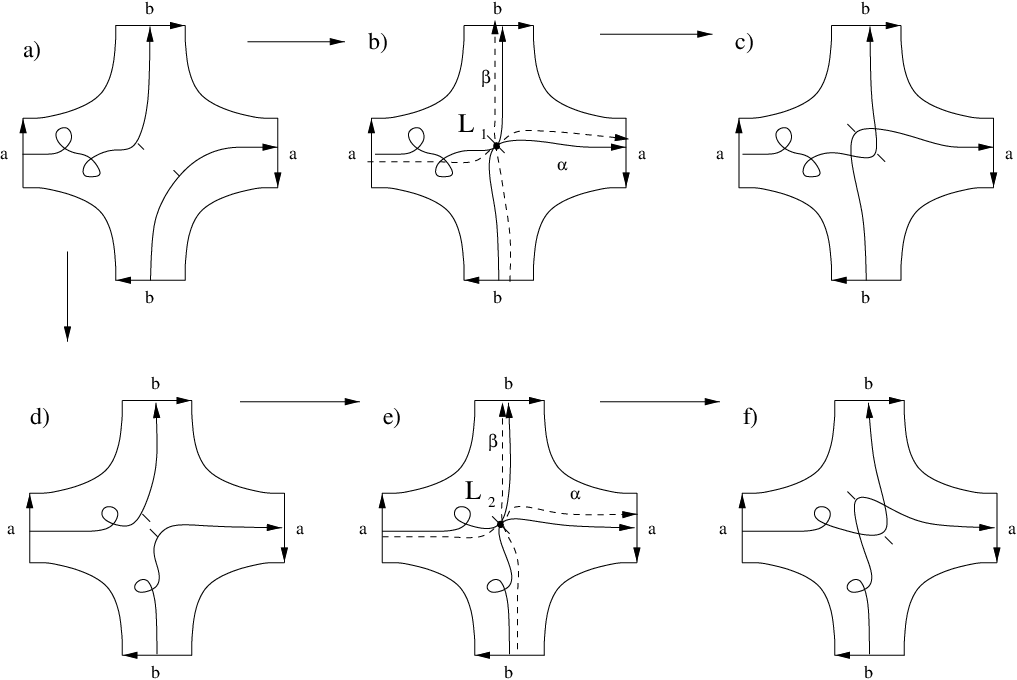
Similarly a front with a safe self-tangency point lifts to a singular Legendrian knot in $PT^{*}F$ . However for nonorientable $F$ it is not true that order one $J^{-}$ -type invariants are order one invariants of Legendrian knots in $PT^{*}F$ . To see this consider a nonorientable surface shown in Figure 10. One can verify that any order one invariant of Legendrian knots in $PT^{*}F$ takes equal values on the Legendrian lifting of fronts shown in Figure 10 c and f, but there exists an order one $J^{-}$ -type invariant which takes different values on the two fronts. To construct such $J^{-}$ -type order one invariant we observe that any function on $\mathcal{K}^{-}_{i}$ is integrable along the loop $\gamma_{1}$ and hence gives rise to an order one $J^{-}$ -type invariant, see Subsection 5.3. Both fronts are obtained from the front in Figure 10 by an isotopy and a (positive) crossing of the $K^{-}$ -stratum. Finally we observe that the fronts $L_{1}$ and $L_{2}$ in Figure 10 b and e realise different $K^{-}_{i}$ -equivalence classes. If one of them is $(\alpha,\beta,0)\in R_{K^{-}}$ , then the second one is $(\alpha f^{2},\beta f^{2},0)\in R_{K^{-}}$ . (Here $f\in\pi_{1}^{-}(PTF)$ is the class of the fiber of $PT^{*}F\rightarrow F$ ). The fact that the two classes are different can be easily obtained from Proposition 8.2.17 and the identities similar to 2 and 3 of Proposition 8.2.6. (Recall that $(f,0)$ does not belong to the group by the action of which we quotient $R_{K^{-}}$ to define the $K^{-}_{i}$ -equivalence relation.) Hence any function on $\mathcal{K}^{-}_{i}$ that takes different values on the $K^{-}_{i}$ -equivalence classes of $L_{1}$ and $L_{2}$ gives rise to the desired invariant.

One can show that the Legendrian liftings of $L_{1}$ and $L_{2}$ can be transformed to each other in the class of Legendrian knots with a double point (so that the points on the parameterizing circle corresponding to the double point change continuously under the transformation). Hence the values of the derivative of any order one invariant of Legendrian knots in $PT^{*}F$ on $L_{1}$ and on $L_{2}$ are equal, and thus the values of the invariant on the Legendrian liftings to $PT^{*}F$ of fronts in Figure 10 c and f are equal.

6. An explicit formula for the finest order one $J^{+}$ -type invariant on orientable $F\neq S^{2}$

Below we give an explicit formula for $I^{+}$ an order one $J^{+}$ -type invariant of generic wave fronts on an orientable surface $F$ . If $F\neq S^{2}$ then the invariant distinguishes every two generic wave fronts that one can distinguish using order one $J^{+}$ -type invariants with values in any Abelian group (not necessarily torsion free), see Theorem 6.0.2.

We assign a positive (resp. negative) sign to a cusp point if the coorienting vector turns in the positive (resp. negative) direction while traversing a small neighborhood of the cusp point along the orientation of the front. We denote half of the number of positive and negative cusp of the front $L$ by $C^{+}$ and $C^{-}$ respectively.

Using the orientation of $F$ one gets that there are four types of double points of a wave front. Two of them are shown in Figure 11, two more are obtained by a change of coorientation on both participating branches. To a double point $d$ of $L$ we correspond two nongeneric fronts $L^{r}_{d},L^{l}_{d}\in K^{+}$ , as it is shown in Figure 11. (The $L^{r}_{d},L^{l}_{d}$ fronts for the double points of the types not shown in the Figure are obtained by a change of coorientation.) We denote by $[L^{r}_{d}],[L^{l}_{d}]$ the $K^{+}$ -equivalence classes of these fronts. The set $\mathcal{K}^{+}$ is naturally identified with the set $R^{+}$ which is the factor of $\pi_{1}(STF)\oplus\pi_{1}(STF)$ modulo the action of $\pi_{1}(STF)$ by conjugation of the first two summands and by the action of ${\mathbb{Z}}_{2}$ permuting the summands.

We denote by ${\mathbb{Z}}[\mathcal{K}^{+}]$ the free ${\mathbb{Z}}$ -module of all formal finite integer combinations of elements of $\mathcal{K}^{+}$ . For a wave front $L$ we denote by $[lf_{2}^{-1},f_{2}]$ , $[l,1]$ , $[lf_{2},f_{2}^{-1}]$ the $K^{+}$ -equivalence classes described by the corresponding elements of $R^{+}$ .

Theorem 6.0.1.

Put $I^{+}(L)\in{\mathbb{Z}}[\mathcal{K}^{+}]$ to be

(5)

\bigl(\sum_{d}([L^{r}_{d}]-[L^{l}_{d}])\bigr)-C^{-}([l,1]-[lf_{2},f_{2}^{-1}])-C^{+}([l,1]-[lf_{2}^{-1},f_{2}]).

Then $I^{+}(L)$ is an order one $J^{+}$ -type invariant. Under the positive crossing of the $K^{+}$ -stratum corresponding to $[s_{1},s_{2}]\in R^{+}$ it increases by $\bigl(2[s_{1},s_{2}]-[s_{1}f_{2},s_{2}f_{2}^{-1}]-[s_{1}f_{2}^{-1},s_{2}f_{2}]\bigr)$ .

The proof of the Theorem is straightforward. One verifies that $I^{+}(L)$ does not change under crossings of $\Lambda$ -, $K^{-}$ -, $\Pi$ -, and $T$ -strata. To see that $I^{+}(L)$ has the described behaviour under the crossings of the $K^{+}$ -stratum, one uses the fact that $f_{2}$ is in the center of $\pi_{1}(STF)$ , see 8.2.6.

(To construct a similar invariant of wave fronts on non-orientable surfaces one symmetrizes the construction of $L^{r}_{d}$ and $L^{l}_{d}$ and gets four elements of $\mathcal{K}^{+}$ corresponding to the double point $d$ .)

The following theorem says that for orientable $F\neq S^{2}$ the invariant $I^{+}$ is the finest order one $J^{+}$ -type invariant.

Theorem 6.0.2.

Let $\mathcal{C}$ be a connected component of the space of fronts on an orientable $F\neq S^{2}$ . Let $L_{1},L_{2}\in\mathcal{C}$ be generic fronts, and $\overline{I^{+}}$ an order one $J^{+}$ -type invariant of fronts with values in some Abelian group $G$ (not necessarily torsion free). Then $\overline{I^{+}}(L_{1})=\overline{I^{+}}(L_{2})$ , provided that $I^{+}(L_{1})=I^{+}(L_{2})$ .

For the proof of Theorem 6.0.2 see Section 11.

It is well known that in the case of $F={\mathbb{R}}^{2}$ the partial linking polynomial of F. Aicardi [2] appears to be the finest order one invariant in the above sense. Other order one $J^{+}$ -type invariants of wave fronts on surfaces were constructed by M. Polyak [15] and by the author in [18]. They are significantly easier for calculation but are not the finest in the above sense.

7. Homotopy groups of the space of fronts

Fix $a\in S^{1}$ , then $L\in\mathcal{L}$ represent an element of $\pi_{1}(F,L(a))$ , the lifting $l$ of $L$ to $STF$ represents an element of $\pi_{1}(STF,l(a))$ , and the lifting $\vec{l}$ of $L$ to $CSTF$ represents an element of $\pi_{1}(CSTF,\vec{l}(a))$ .

7.1. Fundamental group of the space of fronts on an orientable surface.

For orientable surfaces the group $\pi_{1}(\mathcal{L},L)$ appears to be much simpler than for nonorientable surfaces.

Theorem 7.1.1.

Let $F=S^{2}$ and $L$ a front on $S^{2}$ . Then $\pi_{1}(\mathcal{L},L)={\mathbb{Z}}\oplus{\mathbb{Z}}_{2}$ .

Theorem 7.1.2.

Let $F=T^{2}$ (torus) and $L$ a front on $T^{2}$ . Then $\pi_{1}(\mathcal{L},L)={\mathbb{Z}}^{4}$ .

For the proofs of Theorems 7.1.1 and 7.1.2 see Subsection 12.1.

Theorem 7.1.3.

Let $F\neq S^{2},T^{2}$ be an orientable surface (not necessarily compact), and let $L$ be a front on $F$ .

I:: If $L\neq 1\in\pi_{1}(F)$ , then $\pi_{1}(\mathcal{L},L)={\mathbb{Z}}^{3}$ .
II:: If $L=1\in\pi_{1}(F)$ , then $\pi_{1}(\mathcal{L},L)={\mathbb{Z}}\oplus\pi_{1}(STF)$ .

For the proof of Theorem 7.1.3 see Subsection 12.2.

7.2. Fundamental group of the space of fronts on a nonorientable surface

We denote by $\pi_{1}^{pres}(F)$ the subgroup of $\pi_{1}(F)$ consisting of all orientation-preserving loops and by $\pi_{1}^{rev}(F)$ the subset of $\pi_{1}(F)$ which is $\pi_{1}(F)\setminus\pi_{1}^{pres}(F)$ . We denote by $\pi_{1}^{pres}(STF)$ the subgroup of $\pi_{1}(STF)$ which is a preimage of $\pi_{1}^{pres}(F)$ under $\operatorname{pr}^{2}_{*}:\pi_{1}(STF)\rightarrow\pi_{1}(F)$ and by $\pi_{1}^{rev}(STF)$ the subset of $\pi_{1}(STF)$ which is a preimage of $\pi_{1}^{rev}(F)$ under $\operatorname{pr}^{2}_{*}$ . We denote by ${\mathbb{Z}}^{ev}$ the subgroup of even numbers in ${\mathbb{Z}}$ and by ${\mathbb{Z}}^{odd}$ the subset of odd numbers in ${\mathbb{Z}}$ .

Theorem 7.2.1.

Let $F={\mathbb{R}}P^{2}$ and $L$ a front on ${\mathbb{R}}P^{2}$ . Then $\pi_{1}(\mathcal{L},L)$ is isomorphic to ${\mathbb{Z}}\oplus{\mathbb{Z}}_{2}$ .

Theorem 7.2.2.

Let $F=K$ (Klein bottle), and let $L$ be a front on $K$ .

I:: If $L\in\pi_{1}^{pres}(K)$ , then

a: $\pi_{1}(\mathcal{L},L)$ is isomorphic to ${\mathbb{Z}}\oplus\pi_{1}(STK)$ , provided that $l=b^{2k}\in\pi_{1}(STK,l(a))$ for some $b\in\pi_{1}^{rev}(STK,l(a))$ .

b: $\pi_{1}(\mathcal{L},L)={\mathbb{Z}}^{4}$ otherwise.
II:: If $L\in\pi_{1}^{rev}(K)$ , then $\pi_{1}(\mathcal{L},L)$ is isomorphic to ${\mathbb{Z}}^{2}$ .

For the proofs of Theorems 7.2.1 and 7.2.2 see Subsection 12.1.

Let $F\neq{\mathbb{R}}P^{2},K$ be a nonorientable surface (not necessarily compact), and let $L$ be a front on $F$ such that $L\neq 1\in\pi_{1}(F,L(a))$ . One can show that there exists a unique maximal Abelian subgroup $G_{L}<\pi_{1}(F,L(a))$ containing $L\in\pi_{1}(F,L(a))$ , and that this $G_{L}$ is isomorphic to ${\mathbb{Z}}$ (see also Proposition 8.2.17). Let $g$ be a generator of $G_{L}$ and $L_{g}$ a front such that $\vec{l}_{g}(a)=\vec{l}(a)$ and $L_{g}=g\in\pi_{1}(F,L(a))$ . One can show that $l\in\pi_{1}(STF,l(a))$ can be presented in the unique way as $l_{g}^{k}f_{2}^{m}\in\pi_{1}(STF,l(a))$ (see also the Proof of Theorem 7.2.3).

Theorem 7.2.3.

Let $F\neq{\mathbb{R}}P^{2},K$ be a nonorientable surface (not necessarily compact), and let $L$ be a front on $F$ .

I:: If $L\in\pi_{1}^{rev}(F)$ , then $\pi_{1}(\mathcal{L},L)$ is isomorphic to ${\mathbb{Z}}^{2}$ .
II:: If $L\in\pi_{1}^{pres}(F)$ and $L\neq 1\in\pi_{1}(F)$ , then:

a: $\pi_{1}(\mathcal{L},L)$ is isomorphic to ${\mathbb{Z}}\oplus\pi_{1}(K)$ , provided that $L_{g}\in\pi_{1}^{rev}(F)$ and that $l=l_{g}^{2k}\in\pi_{1}(STF,l(a))$ , for some $k\in{\mathbb{Z}}$ .

b: $\pi_{1}(\mathcal{L},L)={\mathbb{Z}}^{3}$ otherwise.
III:: If $L=1\in\pi_{1}(F)$ , then:

a: $\pi_{1}(\mathcal{L},L)$ is isomorphic to ${\mathbb{Z}}\oplus\pi_{1}^{pres}(STF)$ , provided that $l\neq 1\in\pi_{1}(STF)$ .

b: $\pi_{1}(\mathcal{L},L)$ is isomorphic to the subgroup of ${\mathbb{Z}}\oplus\pi_{1}(STF)$ which is $({\mathbb{Z}}^{even}\oplus\pi_{1}^{pres}(STF))\cup({\mathbb{Z}}^{odd}\oplus\pi_{1}^{rev}(STF))$ , provided that $l=1\in\pi_{1}(STF)$ .

For the proof of Theorem 7.2.3 see Subsection 12.2.

Statement III.a (resp. III.b) corresponds to $L$ that is regular homotopic to one of the fronts of type $K_{i,k}$ , $i>0$ , (resp. of type $K_{0,k}$ ) see Figure 5.

7.3. Higher homotopy groups of the space of fronts.

Theorem 7.3.1.

Let $F$ be a surface (not necessarily compact or orientable) and let $L$ be a front on $F$ .

I:: If $F$ is $S^{2}$ or ${\mathbb{R}}P^{2}$ , then $\pi_{2}(\mathcal{L},L)={\mathbb{Z}}$ , and $\pi_{n}(\mathcal{L},L)=\pi_{n}(S^{2})\oplus\pi_{n+1}(S^{2})$ , $n\geq 3$ .
II:: If $F\neq S^{2},{\mathbb{R}}P^{2}$ , then $\pi_{n}(\mathcal{L},L)=0$ , $n\geq 2$ .

For the Proof of Theorem 7.3.1 see Section 12.3.

8. Proof of Theorem 4.2.1

We prove only the statements of Theorem 4.2.1 related to the existence of the $\overline{\operatorname{St}^{\prime}}$ invariant integrating $\psi_{1}$ in $\mathcal{C}$ . The proofs of statements related to the existence of $\overline{J^{+}}$ and $\overline{J^{-}}$ invariants are obtained in a similar way.

In order for $\overline{\operatorname{St}^{\prime}}$ to be well defined, the change of it along any generic loop has to be zero. This proves the necessity of the conditions described in Theorem 4.2.1. Let us prove that these conditions are sufficient for the existence of $\overline{\operatorname{St}^{\prime}}$ invariant integrating $\psi_{1}$ in $\mathcal{C}$ .

Put $\overline{\operatorname{St}^{\prime}}(L)$ to be any number. Let $L^{\prime}\in\mathcal{C}$ be a generic front and $p$ a generic path connecting $L$ to $L^{\prime}$ . Similarly to the case of a closed loop we define $\Delta_{\overline{\operatorname{St}^{\prime}}}(p)$ . Put $\overline{\operatorname{St}^{\prime}}(L^{\prime})=\overline{\operatorname{St}^{\prime}}(L)+\Delta_{\overline{\operatorname{St}^{\prime}}}(p)$ . To prove the theorem it suffices to show that $\overline{\operatorname{St}^{\prime}}(L^{\prime})$ is independent of the generic path $p$ which was used to define it. The last statement follows from Lemmas 8.0.1 and 8.0.2. Thus we proved Theorem 4.2.1 modulo these two lemmas. ∎

Lemma 8.0.1 (Cf. Arnold [5]).

Let $p$ be a generic path in $\mathcal{C}$ connecting $L$ to itself. Then $\Delta_{\overline{\operatorname{St}^{\prime}}}(p)$ depends only on the element of $\pi_{1}(\mathcal{C},L)$ realized by $p$ .

Lemma 8.0.2.

Let $F$ be a surface, $\mathcal{C}$ a connected component of $\mathcal{L}$ , and $\psi_{1}:\mathcal{T}\rightarrow{\mathbb{Z}}$ a function integrable along those of the loops $\gamma_{1}$ and $\gamma_{2}$ that participate in the statement of Theorem 4.2.1 corresponding to $F$ and $\mathcal{C}$ . Then every $\alpha\in\pi_{1}(\mathcal{C},L)$ can be realized by a generic loop $q_{\alpha}$ in $\mathcal{C}$ such that $\Delta_{\overline{\operatorname{St}^{\prime}}}(q_{\alpha})=0$ .

8.1. Proof of Lemma 8.0.1

To prove the Lemma, it suffices to show that if we go around any codimension two stratum of the discriminant along a small generic loop $r$ (not necessarily starting at $L$ ), then $\Delta_{\overline{\operatorname{St}^{\prime}}}(r)=0$ . All the codimension two strata are described in the following Theorem.

Theorem 8.1.1 (Arnold [5]).

The strata of codimension two of the discriminant of $\mathcal{L}$ are formed by fronts with two nongeneric singular points that are singular of codimension one, and by fronts with one nongeneric singular point that is one of the following (see Figure 12 and Figure 13):

1) A quadruple point with pairwise transverse tangent lines. This stratum is denoted by $TT$ .

2) A cusp passing through a branch in such a way that they have the same tangent line. This stratum is denoted by $K\Pi$ .

3) A degenerate triple point at which two branches are tangent of order one and the third branch is transverse to them. This stratum is denoted by $KT$ .

4) A point of a cubical self-tangency. This stratum is denoted by $KK$ .

5) A cusp point passing simultaneously through two branches. (Here it is assumed that the lines tangent to the three participating branches are different.) This stratum is denoted by $T\Pi$ .

6) A point of degree $\frac{4}{3}$ passing through a branch of the front. (Here it is assumed that the two branches have transverse tangent lines.) This stratum is denoted by $\Pi\Lambda$ .

7) Two coinciding cusp points. (Here it is assumed that the lines tangent to the two branches are different.) This stratum is denoted by $\Pi\Pi$ .

8) A point of degree $\frac{5}{4}$ . This stratum is denoted by $\Lambda\Lambda$ .

8.1.2.

The only strata of the discriminant of codimension two in whose bifurcation diagram triple points or cusp crossings are present are: two distinct codimension one singular points one of which is a triple point; two distinct codimension one singular points one of which is a cusp crossing point; and strata $TT$ , $KT$ , $K\Pi$ , $T\Pi$ , $\Pi\Pi$ , $\Pi\Lambda$ and $\Lambda\Lambda$ (in the notation of Lemma 8.1.1).

If $r$ is a small loop going around a stratum of two distinct codimension one singular points one of which is a cusp or a triple point, then in $\Delta_{\overline{\operatorname{St}^{\prime}}}(r)$ we have each of the participating $T$ -equivalence classes twice, once with the plus sign of the newborn vanishing triangle, once with the minus. Hence $\Delta_{\overline{\operatorname{St}^{\prime}}}(r)=0$ .

To prove the statement for the other strata we use the bifurcation diagrams shown in Figure 12 and Figure 13.

Let $r$ be a small loop going around the $TT$ -stratum. We can assume that it corresponds to a loop in Figure 14 directed counterclockwise. There are eight terms in $\Delta_{\overline{\operatorname{St}^{\prime}}}(r)$ . We split them into pairs I, II, III, IV, as it is shown in Figure 14. One can see that the wave fronts from the same pair are $T$ -equivalent. For each branch the sign of the colored triangle is equal to the sign of the triangle that died under the $T$ -stratum crossing shown on the next (in the counterclockwise direction) branch. The sign of the dying vanishing triangle is minus the sign of the newborn vanishing triangle. Finally, one can see that the signs of the colored triangles inside each pair are opposite. Thus all these eight terms cancel out, and $\Delta_{\overline{\operatorname{St}^{\prime}}}(r)=0$ .

There are six terms in $\Delta_{\overline{\operatorname{St}^{\prime}}}(r)$ for $r$ a loop going around the $T\Pi$ -stratum. Two of them correspond to $r$ crossing the $T$ -stratum, and four to $r$ crossing the $\Pi$ -stratum. One verifies that the two terms corresponding to $r$ crossing the $T$ -stratum cancel out. We split the other four terms into pairs such that the terms in a pair correspond to the cusp crossing the same branch of the front. One verifies that the $T$ -equivalence classes inside a pair coincide and the signs of the terms are opposite. Thus the terms inside each pair cancel out.

In a similar way one show that $\Delta_{\overline{\operatorname{St}^{\prime}}}(r)=0$ for a small loop $r$ going around $K\Pi$ -, $KT$ -, $\Pi\Pi$ -, and $\Lambda\Lambda$ -strata.

Finally, let $r$ be a loop going around the $\Pi\Lambda$ -stratum. There are three terms in $\Delta_{\overline{\operatorname{St}^{\prime}}}(r)$ . One of them corresponds to $r$ crossing the $T$ -stratum and two to $r$ crossing the $\Pi$ -stratum. One verifies that that the sign of the crossing of the $T$ -stratum is opposite from the signs of the crossings of the $\Pi$ -stratum, and that all three $T$ -equivalence classes are the same. We denote the class by $t$ . Thus, $\Delta_{\overline{\operatorname{St}^{\prime}}}(r)=\frac{1}{2}\psi(t)+\frac{1}{2}\psi(t)-\psi(t)=0$ .

Remark 8.1.3.

Recall that the magnitude of the change of $\operatorname{St}^{\prime}$ under the crossing of the part of the $\Pi$ -stratum corresponding to the $T$ -equivalence class $t$ was put to be $\frac{1}{2}\psi(t)$ . One can see that if we substitute $\frac{1}{2}$ by another constant, then there is no hope for constructing an invariant of this sort, unless $\psi$ is zero on all the $T$ -equivalence classes appearing on the $\Pi$ -stratum.

This finishes the Proof of Lemma 8.0.1. ∎

8.2. Constructions and facts needed for the proof of Lemma 8.0.2

8.2.1.

Parametric $h$ -principle. The parametric $h$ -principle proved for the Legendrian curves by M. Gromov [8] says that the space of wave fronts $\mathcal{L}$ is weak homotopy equivalent to the space $\Omega CSTF$ of all free loops in $CSTF$ , see 2.1. The mapping $h:\mathcal{L}\rightarrow\Omega CSTF$ that gives the equivalence sends a wave front $L$ (corresponding to the Legendrian curve $l$ ) to the loop $\vec{l}\in\Omega CSTF$ .

Fix $a\in S^{1}$ . Let $q$ be a loop in $\mathcal{L}$ starting at $L$ . At any moment of time $q(t)$ is a wave front that can be lifted to a loop in $CSTF$ . Thus $q$ gives rise to the mapping $q_{h}:S^{1}\times S^{1}\rightarrow CSTF$ . (In the product $S^{1}\times S^{1}$ the first copy of $S^{1}$ corresponds to the parameterization of a front and the second to the parameterization of the loop $q$ .) The mapping $q_{h}$ restricted to $a\times S^{1}$ is a loop $t_{a}(q)$ in $CSTF$ . One can verify that the mapping $t_{a}:\pi_{1}(\mathcal{L},L)\rightarrow\pi_{1}(CSTF,\vec{l}(a))$ is a homomorphism.

Proposition 8.2.2.

$t_{a}:\pi_{1}(\mathcal{L},L)\rightarrow\pi_{1}(CSTF,\vec{l}(a))$ is an isomorphism of $\pi_{1}(\mathcal{L},L)$ onto the centralizer $Z(\vec{l})$ of $\vec{l}\in\pi_{1}(CSTF,\vec{l}(a))$ .

8.2.3.

Proof of Proposition 8.2.2. Let $p:\Omega CSTF\rightarrow CSTF$ be the mapping that sends $\omega\in\Omega CSTF$ to $\omega(a)\in CSTF$ . (One can verify that this $p$ is a Serre fibration, with the fiber of it over a point isomorphic to the space of loops based at the point.) The $h$ -principle (see 8.2.1) implies that to prove the Proposition it suffices to show that $p_{*}:\pi_{1}(\Omega CSTF,\vec{l})\rightarrow\pi_{1}(CSTF,\vec{l}(a))$ is an isomorphism of $\pi_{1}(\Omega CSTF,\vec{l})$ onto $Z(\vec{l})$ .

A Proposition proved by V.L. Hansen [9] says that if $X$ is a topological space with $\pi_{2}(X)=0$ , then $\pi_{1}(\Omega X,\omega)=Z(\omega)<\pi_{1}(X,\omega(a))$ . (Here $\Omega X$ is the space of free loops in $X$ and $\omega$ is an element of $\Omega X$ .) One can verify that $\pi_{2}(CSTF)=0$ for any surface $F$ . Thus, $\pi_{1}(\Omega CSTF,\vec{l})$ is isomorphic to $Z(\vec{l})<\pi_{1}(CSTF,\vec{l}(a))$ . From the proof of the Hansen’s Proposition it follows that the isomorphism is given by $p_{*}$ . ∎

Proposition 8.2.4.

The fiberwise projectivization $PCSTF$ of $CSTF$ is isomorphic to $S^{1}\times STF$ .

8.2.5.

Proof of Proposition 8.2.4. A local orientation at $x\in F$ induces an orientation of the $S^{1}$ -fiber of $STF$ over $x$ , which changes if we change the local orientation at $x$ . Hence $STF$ is canonically oriented. The planes of the contact structure of $STF$ are canonically cooriented. Thus they are also canonically oriented. The orientations of them induce a coherent orientation of the ${\mathbb{R}}P^{1}$ -fibers of $PCSTF\rightarrow STF$ . Hence to prove the proposition it suffices to construct a section of $PCSTF$ over $STF$ .

A point $x\in STF$ is described by $\operatorname{pr}_{2}(x)\in F$ and a cooriented contact element at $\operatorname{pr}_{2}(x)$ . Consider an arc $L_{x}$ of the geodesic passing through $\operatorname{pr}_{2}(x)$ that is tangent to the contact element. Equip the arc with the coorientation coherent with the one of the contact element. Choose an orientation of $L_{x}$ and lift it to an immersed arc in $STF$ . The direction of $l_{x}$ at the lifting of the preimage of $\operatorname{pr}_{2}(x)$ defines a point in the $S^{1}$ -fiber of $CSTF$ over $x$ and, consequently, a point $\bar{x}$ in the ${\mathbb{R}}P^{1}$ -fiber of $PCSTF$ over $x$ . Clearly the point $\bar{x}$ in the ${\mathbb{R}}P^{1}$ -fiber is independent of the choice of the orientation of $L_{x}$ . The desired section is given by mapping $x\in STF$ to the point $\bar{x}\in PCSTF$ . ∎

Proposition 8.2.6.

Let $f_{1}\in\pi_{1}(CSTF,\vec{l}(a))$ and $f_{2}\in\pi_{1}(STF,l(a))$ be the classes of oriented (in some way) fibers of the $S^{1}$ -fibrations $\operatorname{pr}^{1}:CSTF\rightarrow STF$ and $\operatorname{pr}^{2}:STF\rightarrow F$ respectively. Then:

1. $f_{1}\alpha=\alpha f_{1}\in\pi_{1}(CSTF,\vec{l}(a)$ for any $\alpha\in\pi_{1}(CSTF,\vec{l}(a))$ .

2. $f_{2}\alpha=\alpha f_{2}\in\pi_{1}(STF,l(a))$ for any $\alpha\in\pi_{1}(STF,l(a))$ projecting to an orientation-preserving loop in $F$ .

3. $f_{2}\alpha=\alpha f_{2}^{-1}\in\pi_{1}(STF,l(a))$ for any $\alpha\in\pi_{1}(STF,l(a))$ projecting to an orientation-reversing loop in $F$ .

8.2.7.

Proof of Proposition 8.2.6. Consider the double covering $p:CSTF\rightarrow PCSTF$ . The homomorphism $p_{*}:\pi_{1}(CSTF)\rightarrow\pi_{1}(PCSTF)$ is injective, and it maps $f_{1}$ to $f^{2}\in\pi_{1}(PCSTF)$ . (Here $f$ is the class of an oriented $S^{1}$ -fiber of $PCSTF\rightarrow STF$ .) Proposition 8.2.4 implies that $f$ is in the center of $\pi_{1}(PCSTF)$ , and we have proved the first statement of the proposition.

If we move an oriented fiber along the loop $\alpha\subset STF$ , then in the end it comes to itself either with the same or with the opposite orientation. Thus for any $\alpha\in\pi_{1}(STF,l(a))$ either $f_{2}\alpha=\alpha f_{2}$ or $f_{2}\alpha=\alpha f_{2}^{-1}$ . A local orientation of the neighborhood of a point in $F$ induces an orientation of the fiber of $\operatorname{pr}^{2}$ over the point. Combining these facts we get the proof of the other two statements of the proposition. ∎

Proposition 8.2.8.

For any $\alpha\in\pi_{1}(CSTF,d)$ there exists a Legendrian curve $l$ such that $\vec{l}(a)=d$ and $\vec{l}=\alpha\in\pi_{1}(CSTF,d)$ .

8.2.9.

Proof of Proposition 8.2.8. Let $L$ be a front such that $\vec{l}(a)=d$ and $L=\operatorname{pr}^{2}_{*}\operatorname{pr}^{1}_{*}(\alpha)\in\pi_{1}(F,\operatorname{pr}^{2}\operatorname{pr}^{1}(d))$ . A small extra kink on $L$ corresponds to the multiplication of $l\in\pi_{1}(STF)$ by $f_{2}^{\pm 1}$ depending on the side of front the kink points to. Thus, adding extra kinks we can modify $L$ , so that $l=\operatorname{pr}^{1}_{*}(\alpha)\in\pi_{1}(STF)$ . In [5] it is shown that an extra pair of adjacent cusps pointing to opposite sides of a planar front $L_{1}$ corresponds to the multiplication of $\vec{l}_{1}$ by $f_{1}^{\pm 1}$ depending on the sign of the cusps. Since the addition of the pair of cusps is done locally and $f_{2}$ is in the center of $\pi_{1}(CSTF)$ for any $F$ (see 8.2.6), this fact is true for any surface $F$ . Thus we can modify $L$ so that $\vec{l}=\alpha\in\pi_{1}(CSTF,d)$ , and we have proved the proposition.∎

Proposition 8.2.10.

The group $\pi_{1}(CSTF)$ is isomorphic to the index two subgroup of $\pi_{1}(PCSTF)=\pi_{1}(S^{1})\oplus\pi_{1}(STF)={\mathbb{Z}}\oplus\pi_{1}(STF)$ consisting of elements of the form (odd number, element projecting to an orientation-reversing loop in $F$ ) and (even number, element projecting to an orientation-preserving loop in $F$ ).

8.2.11.

Proof of Proposition 8.2.10. By proposition 8.2.8 an element of $\pi_{1}(CSTF)$ can be realized as a lifting $\vec{l}$ of some front $L$ . Orientation-preserving fronts have even number of cusps, and orientation-reversing fronts have odd number of cusps. There are only two (opposite) points in the $S^{1}$ -fiber of $\operatorname{pr}^{1}:CSTF\rightarrow STF$ over $x$ corresponding to a cusp point of a front at $x$ . (These points are identified under $p:CSTF\rightarrow PCSTF$ .) Thus for $\alpha\in\pi_{1}(CSTF)$ the projection of $p_{*}(\alpha)\in\pi_{1}(PCSTF)={\mathbb{Z}}\oplus\pi_{1}(STF)$ to the ${\mathbb{Z}}$ -summand is even provided that $\operatorname{pr}^{2}\operatorname{pr}^{1}(\alpha)$ is an orientation-preserving loop in $F$ and odd otherwise. The difference between the projections of $p_{*}(\alpha)$ and $p_{*}(\alpha f_{1})$ to the ${\mathbb{Z}}$ -summand in $\pi_{1}(PCSTF)$ is two. Since $\pi_{1}(CSTF)$ is isomorphic to $p_{*}(\pi_{1}(CSTF))<\pi_{1}(PCSTF)$ we get the statement of the proposition.∎

8.2.12.

Loop $\gamma_{3}$ . Let $\mathcal{C}$ be a connected component of $\mathcal{L}$ and $L\in\mathcal{C}$ a generic front. Let $\gamma_{3}\in\pi_{1}(\mathcal{L},L)$ be the loop constructed below.

Deform $L$ along a generic path $t$ in $\mathcal{C}$ , so that all cusps are concentrated on a small piece $P$ of $L$ and the side of $L$ they point to alternates. (The notion of side is locally well defined.) This is possible because we can cancel a pair of adjacent cusps pointing to the same side of $L$ , see Figure 15.

If after this deformation the number of cusps is nonzero, then we take the last pair of cusps in $P$ and slide them along $L$ till they come to the beginning of $P$ . Then we shift all the cusps by two positions, so that $L$ gets the shape it had before the sliding. (If $L$ is an orientation-reversing front, then it can happen that there is only one cusp on $P$ . Then to obtain $\gamma_{3}$ we slide the cusp twice around $L$ till it comes to the original position.) We require the deformation to be such that at each moment of time points of $L$ located outside of a small neighborhood of participating cusps do not move.

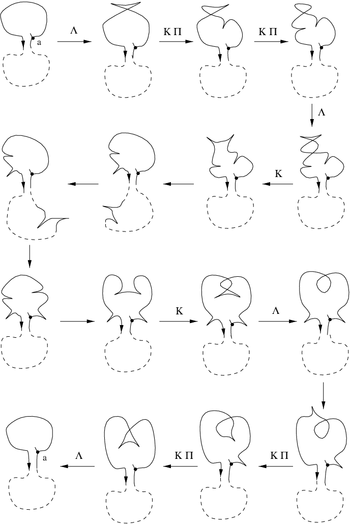
If after the deformation the number of cusps is zero (this happens if $\mu(L)=0$ ), then we perform a regular homotopy shown in Figure 16.

Finally we deform $L$ to its original shape along $t^{-1}$ .

Proposition 8.2.13.

1. Let $L$ be an orientation preserving front on $F$ , then $\operatorname{pr}_{*}^{1}(t_{a}(\gamma_{1}))=f_{2}^{\pm 1}\in\pi_{1}(STF,l(a))$ . (Here the sign of the power of $f_{2}$ depends on the orientation of the fiber we choose to define $f_{2}$ .)

2. Let $L$ be a front on $F$ , then $t_{a}(\gamma_{3})=f_{1}^{\pm 1}\in\pi_{1}(CSTF,\vec{l}(a))$ . (Here the sign of the power of $f_{1}$ depends on the orientation of the fiber we choose to define $f_{1}$ .)

8.2.14.

Proof of Proposition 8.2.13. Under the deformation of $L$ described by $\gamma_{1}$ the point $L(a)$ never leaves a small neighborhood of its original position, and the coorienting normal to $L$ at $L(a)$ is rotated by $2\pi$ . (The rotation happens when the kink passes through $L(a)$ .) Thus the trajectory of $a$ under the lifting of $\gamma_{1}$ to a loop in the space of Legendrian curves represents a class of the fiber of the fibration $\operatorname{pr}^{2}$ . Clearly, this trajectory coincides with $\operatorname{pr}^{1}_{*}(t_{a}(\gamma_{1}))$ and we have proved the first statement of the Proposition.

From 8.2.6 we know that $f_{1}$ is in the center of $\pi_{1}(CTSF)$ . Hence to prove the second statement it suffices to prove the corresponding fact for a loop that is free homotopic to $\gamma_{3}$ . Thus we can assume that under the deformation $\gamma_{3}$ the point $L(a)$ never leaves a small neighborhood of its original position, and that $L$ has the property that all cusps of it are close to each other (in $L$ ), and the side of $L$ they point to alternates. (The notion of side is locally well defined.)

One verifies that under $\gamma_{3}$ the total rotation angle of the coorienting normal at $L(a)$ is zero. Thus the trajectory of $a$ under the lifting of $\gamma_{3}$ to a loop in the space of Legendrian curves in $STF$ represents $1\in\pi_{1}(STF,l(a))$ . Hence $t_{a}(\gamma_{3})=f_{1}^{k}\in\pi_{1}(CSTF,\vec{l}(a))$ , for some $k\in{\mathbb{Z}}$ . We have to show that $k=\pm 1$ .

One verifies that there are only two points in the $S^{1}$ -fiber of $CSTF$ over $l(a)$ which correspond to the front having a cusp at $L(a)$ . A lemma proved by Arnold [5] says that under the deformations of the wave front shown in Figure 17 the velocity vector at the point $l(a)$ is turning in the direction dependent only on, whether it is true or not, that after the deformation the coorienting normal is pointing to the same direction as the curvature vector. (In Figure 17 the marked point is frozen into the surface together with the coorienting normal at it.)

It is clear that the loop $\gamma_{3}$ is free homotopic to $\gamma_{3}^{\prime}$ , in which the point $L(a)$ is frozen into $F$ together with the coorienting normal at it. Under the deformation described by $\gamma_{3}^{\prime}$ the pair of cusps passes through $L(a)$ in the way shown in Figure 18. Using Arnold’s lemma one verifies that under $\gamma_{3}^{\prime}$ the direction of the velocity vector of $l$ at $l(a)$ is rotated by the fiber of $\operatorname{pr}^{1}$ .

This finishes the proof of the Proposition. ∎

Proposition 8.2.15.

$\Delta_{\overline{\operatorname{St}^{\prime}}}(\gamma_{3})=0$ .

8.2.16.

Proof of Proposition 8.2.15. Clearly, the input into $\Delta_{\overline{\operatorname{St}^{\prime}}}$ of the deformation $r$ of $L$ to a front with cusps pointing to alternating (locally well defined) sides of $L$ cancels out with the input into $\Delta_{\overline{\operatorname{St}^{\prime}}}$ of the deformation along $r^{-1}$ .

Consider the case when $\mu(L)\not\in\{0,\pm 1\}$ . No $T$ -stratum crossings occur under the sliding of two cusps and the only inputs into $\Delta_{\overline{\operatorname{St}^{\prime}}}(\gamma_{3})$ come from the crossings of the $\Pi$ -stratum. They occur only when a cusp passes through a neighborhood of a double point $x$ of $L$ , see Figure 19. One verifies that for each double point $x$ the input corresponding to the first cusp passing through the neighborhood of $x$ cancels with the input corresponding to the second cusp passing through it.

If $\mu(L)=0$ , then there are extra crossings of the $\Pi$ -stratum, which occur when we create (and later cancel) two pairs of cusps, one of which slides along $L$ . One verifies that the inputs of these extra crossings cancel out.

If $\mu(L)=\pm 1$ , then $L$ is orientation-reversing, and the only cusp present on $L$ slides twice along $L$ under $\gamma_{3}$ . The input corresponding to the crossings of the $\Pi$ -stratum that occur in the neighborhood of a double point $x$ under the first round of sliding cancels with the input under the second round of sliding. This finishes the proof of Proposition 8.2.15.∎

Proposition 8.2.17.

Let $F\neq S^{2},T^{2}\text{ (torus), }{\mathbb{R}}P^{2},K\text{ (Klein bottle)}$ be a surface (not necessarily compact or orientable), and let $G$ be a nontrivial commutative subgroup of $\pi_{1}(F)$ . Then $G$ is infinite cyclic and there exists a unique maximal infinite cyclic $G^{\prime}<\pi_{1}(F)$ containing $G$ .

8.2.18.

Proof of Proposition 8.2.17. It is well known that any closed $F$ , other than $S^{2},T^{2},{\mathbb{R}}P^{2},K$ , admits a hyperbolic metric of a constant negative curvature. (It is induced from the universal covering of $F$ by the hyperbolic plane $H$ .) The Theorem by A. Preissman (see [6] pp. 258-265) says that if $M$ is a compact Riemannian manifold with a negative curvature, then any nontrivial Abelian subgroup $G<\pi_{1}(M)$ is isomorphic to ${\mathbb{Z}}$ . Thus if $F\neq S^{2},T^{2},{\mathbb{R}}P^{2},K$ is closed, then any nontrivial commutative $G<\pi_{1}(F)$ is infinite cyclic.

The proof of the Preissman’s Theorem given in [6] is based on the fact, that if $\alpha,\beta\in\pi_{1}(M)$ are nontrivial commuting elements, then there exists a geodesic in $\bar{M}$ (the universal covering of $M$ ) which is mapped to itself under the action of these elements considered as deck transformations on $\bar{M}$ . Moreover, these transformations restricted to the geodesic act as translations. This implies that if $F\neq S^{2},T^{2},{\mathbb{R}}P^{2},K$ is a closed surface, then there exists a unique maximal infinite cyclic $G^{\prime}<\pi_{1}(F)$ containing $G$ . This gives the proof of Proposition 8.2.17 for closed $F$ .

If $F$ is not closed, then the statement of the Proposition is also true because in this case $F$ is homotopy equivalent to a bouquet of circles. ∎

8.3. Proof of Lemma 8.0.2

The proof is based on the constructions and the propositions of Subsection 8.2. We start by making the following observation.

8.3.1.

In ${\mathbb{Z}}$ there are no elements of finite order. Thus if $m\neq 0$ , then $\Delta_{\overline{\operatorname{St}^{\prime}}}(q)\neq 0\Leftrightarrow m\Delta_{\overline{\operatorname{St}^{\prime}}}(q)=\Delta_{\overline{\operatorname{St}^{\prime}}}(q^{m})\neq 0$ . Hence, to prove Lemma 8.0.2 it suffices to show that $\Delta_{\overline{\operatorname{St}^{\prime}}}(q^{m})=0$ , for some $m\neq 0$ .

Proposition 8.3.2.

Let $q_{1},q_{2}\in\pi_{1}(\mathcal{L},L)$ be loops such that:

(6)

\operatorname{pr}_{*}^{1}(t_{a}(q_{1}))=\operatorname{pr}_{*}^{1}(t_{a}(q_{2}))\in\pi_{1}(STF,l(a))

Then $\Delta_{\overline{\operatorname{St}^{\prime}}}(q_{2})=\Delta_{\overline{\operatorname{St}^{\prime}}}(q_{1})$ .

8.3.3.

Proof of the Proposition 8.3.2. We know (see 8.2.13) that $t_{a}(\gamma_{3})=f_{1}$ (for a proper choice of an orientation of the fiber used to define $f_{1}$ ). The kernel of the homomorphism $\operatorname{pr}^{1}_{*}$ is generated by $f_{1}$ , which is in the center of $\pi_{1}(CSTF,\vec{l}(a))$ , see 8.2.6. Thus $t_{a}(q_{2})=t_{a}(q_{1})f_{1}^{j}$ for some $j\in{\mathbb{Z}}$ . Proposition 8.2.2 implies that $q_{2}=q_{1}\gamma_{3}^{j}$ . Proposition 8.2.15 says that $\Delta_{\overline{\operatorname{St}^{\prime}}}(\gamma_{3})=0$ . Hence $\Delta_{\overline{\operatorname{St}^{\prime}}}(q_{1})=\Delta_{\overline{\operatorname{St}^{\prime}}}(q_{2})$ . ∎

We first prove Lemma 8.0.2 for $F\neq S^{2},{\mathbb{R}}P^{2},T^{2},K$ , and then separately for the cases of $F=S^{2},{\mathbb{R}}P^{2},T^{2},K$ .

8.3.4.

Case $F\neq S^{2},T^{2},{\mathbb{R}}P^{2},K$ . Proposition 8.2.2 says that $\pi_{1}(\mathcal{L},L)=Z(\vec{l})<\pi_{1}(CSTF,\vec{l}(a))$ . The corresponding isomorphism (see Section 8.2.1) maps $q\in\pi_{1}(\mathcal{L},L)$ to $t_{a}(q)\in\pi_{1}(CSTF,\vec{l}(a))$ . Thus for any $q\in\pi_{1}(\mathcal{L},L)$ the elements $t_{a}(q)$ and $\vec{l}$ commute in $\pi_{1}(CSTF,\vec{l}(a))$ . Hence $L=\operatorname{pr}^{2}_{*}\operatorname{pr}^{1}_{*}(\vec{l})$ commutes with $\operatorname{pr}^{2}_{*}\operatorname{pr}^{1}_{*}(t_{a}(q))$ in $\pi_{1}(F,L(a))$ . Proposition 8.2.17 implies that there exists an isomorphic to ${\mathbb{Z}}$ subgroup of $\pi_{1}(F,L(a))$ generated by some $g\in\pi_{1}(F,L(a))$ that contains both of these loops. Then $L=g^{m}$ and $\operatorname{pr}^{2}_{*}\operatorname{pr}^{1}_{*}(t_{a}(q))=g^{n}$ , for some $m,n\in{\mathbb{Z}}$ .

Consider a wave front $L_{1}$ such that $\vec{l}_{1}(a)=\vec{l}(a)$ , and $g=L_{1}\in\pi_{1}(F,L(a))$ . The kernel of $\operatorname{pr}_{*}^{2}$ is generated by $f_{2}$ which has infinite order in $\pi_{1}(STF)$ for our surfaces $F$ . Proposition 8.2.6 allows us to interchange $f_{2}$ with the other elements of $\pi_{1}(STF,l(a))$ . Thus $l=l_{1}^{m}f_{2}^{i}$ , and $\operatorname{pr}^{1}_{*}(t_{a}(q))=l_{1}^{n}f_{2}^{j}$ (in $\pi_{1}(STF)$ ) for some $i,j\in{\mathbb{Z}}$ .

We prove Lemma 8.0.2 separately in the cases of $m\neq 0$ and $m=0$ in respectively Subsubsections 8.3.5 and 8.3.6. (Geometrically these two cases correspond to $L=1\in\pi_{1}(F)$ and $L\neq 1\in\pi_{1}(F)$ respectively.)

8.3.5.

Case $m\neq 0$ . To prove Lemma 8.0.2 it suffices to show that $\Delta_{\overline{\operatorname{St}^{\prime}}}(q^{m})=0$ (see 8.3.1). We do it by constructing $\alpha\in\pi_{1}(\mathcal{L},L)$ such that $\operatorname{pr}_{*}^{1}(t_{a}(\alpha))=\operatorname{pr}_{*}^{1}(t_{a}(q^{m}))$ and $\Delta_{\overline{\operatorname{St}^{\prime}}}(\alpha)=0$ . After this, Proposition 8.3.2 implies the statement of the lemma.

One can show that:

(7)

\operatorname{pr}_{*}^{1}(t_{a}(q^{m}))=l^{n}f_{2}^{k}\text{ for some }k\in{\mathbb{Z}}.

For an orientation-preserving $g$ this follows from the following calculation (which uses 8.2.6):

(8)

\operatorname{pr}_{*}^{1}(t_{a}(q^{m}))=\bigl(\operatorname{pr}_{*}^{1}(t_{a}(q))\bigr)^{m}=(l_{1}^{n}f_{2}^{j})^{m}=(l_{1}^{m}f_{2}^{i})^{n}f_{2}^{jm-ni}=l^{n}f_{2}^{jm-ni}.

(Recall that $\operatorname{pr}^{1}_{*}(t_{a}(q))=l_{1}^{n}f_{2}^{j}$ for some $j\in{\mathbb{Z}}$ , see 8.3.4.)

For an orientation-reversing $g$ this follows from the similar calculation (also based on Proposition 8.2.6).

The fact that $\operatorname{pr}^{1}_{*}(t_{a}(q^{m}))$ commutes with $l$ (since $t_{a}(q^{m})=(t_{a}(q))^{m}\in Z(\vec{l})$ ) and Proposition 8.2.6 imply that $k=0$ in (7), provided that $L$ is an orientation-reversing front.

Consider the case of $L$ being an orientation-preserving front. Proposition 8.2.13 says that $\operatorname{pr}_{*}^{1}(t_{a}(\gamma_{1}))=f_{2}$ (for a proper choice of the orientation of the fiber used to define $f_{2}$ ). Hence $\operatorname{pr}_{*}^{1}(t_{a}(\alpha))=\operatorname{pr}_{*}^{1}(t_{a}(q^{m}))$ for $\alpha\in\pi_{1}(\mathcal{L},L)$ which is: $n$ times sliding of $L$ along itself (induced by a rotation of the parameterizing circle) composed with $\gamma_{1}^{j}$ .

If $L$ is an orientation-reversing front, then as we have shown above $\operatorname{pr}_{*}^{1}(t_{a}(q^{m}))=l^{n}$ . Hence $\operatorname{pr}_{*}^{1}(t_{a}(\alpha))=\operatorname{pr}_{*}^{1}(t_{a}(q^{m}))$ for $\alpha\in\pi_{1}(\mathcal{L},L)$ which is: $n$ times sliding of $L$ along itself (induced by a rotation of the parameterizing circle).

No discriminant crossings occur under the sliding of $L$ along itself, and $\Delta_{\overline{\operatorname{St}^{\prime}}}(\gamma_{1})=0$ by the assumption of the the lemma. Hence $\Delta_{\overline{\operatorname{St}^{\prime}}}(\alpha)=0$ . Proposition 8.3.2 implies that $\Delta_{\overline{\operatorname{St}^{\prime}}}(q^{m})=0$ . Thus, we have proved (see 8.3.1) Lemma 8.0.2 for $F\neq S^{2},{\mathbb{R}}P^{2},T^{2},K$ and $m\neq 0$ .

8.3.6.

Case $m=0$ . If $m=0$ , then $L=1\in\pi_{1}(F,L(a))$ . We want to construct $\alpha\in\pi_{1}(\mathcal{L},L)$ such that $\operatorname{pr}_{*}^{1}(t_{a}(\alpha))=\operatorname{pr}_{*}^{1}(t_{a}(q^{2}))$ and $\Delta_{\overline{\operatorname{St}^{\prime}}}(\alpha)=0$ . (After this the statement follows from 8.3.1 and Proposition 8.3.2.)

For any $q\in\pi_{1}(\mathcal{L},L)$ the projection $\operatorname{pr}^{2}_{*}\operatorname{pr}_{*}^{1}(t_{a}(q^{2}))$ is an orientation-preserving loop in $F$ . A straightforward verification shows that $\alpha$ can be obtained by a composition of $\gamma_{1}^{\pm 1}$ (see 4.1.1) and loops constructed as follows:

Push $L$ into a small disc by a generic regular homotopy $r$ . Slide this small disc along a smooth orientation-preserving curve in $F$ and return $L$ to its original shape along $r^{-1}$ .

Clearly, the inputs of $r$ and $r^{-1}$ into $\Delta_{\overline{\operatorname{St}^{\prime}}}$ cancel out, and no discriminant crossings happen when we slide the small disc (containing $L$ ) along a loop in $F$ . By the assumption of the lemma $\Delta_{\overline{\operatorname{St}^{\prime}}}(\gamma_{1})=0$ . Thus $\Delta_{\overline{\operatorname{St}^{\prime}}}(\alpha)=0$ . Proposition 8.3.2 implies that $\Delta_{\overline{\operatorname{St}^{\prime}}}(q^{2})=0$ , and we have proved (see 8.3.1) Lemma 8.0.2 for $F\neq S^{2},{\mathbb{R}}P^{2},T^{2},K$ .

8.3.7.

Case $F=S^{2}$ . One verifies that $\pi_{1}(STS^{2})=\pi_{1}({\mathbb{R}}P^{3})={\mathbb{Z}}_{2}$ . Thus $\operatorname{pr}_{*}^{1}(t_{a}(q^{2}))=\operatorname{pr}_{*}^{1}(t_{a}(1))=1\in\pi_{1}(STF,l(a))$ , for any $q\in\pi_{1}(\mathcal{L},L)$ . Proposition 8.3.2 implies that $\Delta{\overline{\operatorname{St}^{\prime}}}(q^{2})=0$ . This finishes (see 8.3.1) the proof of Lemma 8.0.2 for $F=S^{2}$ . ∎

8.3.8.

Case $F=T^{2}$ . One verifies that $\pi_{1}(STT^{2})={\mathbb{Z}}\oplus{\mathbb{Z}}\oplus{\mathbb{Z}}$ . As before we fix $q\in\pi_{1}(\mathcal{L},L)$ and construct $\alpha\in\pi_{1}(\mathcal{L},L)$ such that $\operatorname{pr}_{*}^{1}(t_{a}(\alpha))=\operatorname{pr}_{*}^{1}(t_{a}(q))$ .

One verifies that $\alpha$ can be expressed through $\gamma_{1}$ and loops $\gamma_{4}$ and $\gamma_{5}$ that are slidings of $L$ along the unit vector fields parallel to the meridian and longitude of $T^{2}$ respectively.

Since $\Delta_{\overline{\operatorname{St}^{\prime}}}(\gamma_{1})=0$ by the assumption of the Lemma, and no discriminant crossings occur under $\gamma_{4}$ and $\gamma_{5}$ , we get that $\Delta_{\overline{\operatorname{St}^{\prime}}}(\alpha)=0$ . Proposition 8.3.2 implies that $\Delta_{\overline{\operatorname{St}^{\prime}}}(q)=0$ . This finishes the proof of Lemma 8.0.2 for $F=T^{2}$ .∎

8.3.9.

Case $F={\mathbb{R}}P^{2}$ . One verifies that $\pi_{1}(ST{\mathbb{R}}P^{2})={\mathbb{Z}}_{4}$ . Thus $\operatorname{pr}_{*}^{1}(t_{a}(q^{4}))=\operatorname{pr}_{*}^{1}(t_{a}(1))=1\in\pi_{1}(STF,l(a))$ for any $q\in\pi_{1}(\mathcal{L},L)$ . Proposition 8.3.2 implies that $\Delta{\overline{\operatorname{St}^{\prime}}}(q^{4})=0$ . This finishes (see 8.3.1) the proof of Lemma 8.0.2 for $F={\mathbb{R}}P^{2}$ .∎

8.3.10.

Case $F=K$ . Proposition 8.2.2 says that $\pi_{1}(\mathcal{L},L)$ is isomorphic to $Z(\vec{l})<\pi_{1}(CSTK,\vec{l}(a))$ . The kernel of the homomorphism $\operatorname{pr}^{1}_{*}$ is generated by $f_{1}$ which is in the center of $\pi_{1}(CSTF,\vec{l}(a))$ , see 8.2.6. Thus $\operatorname{pr}^{1}_{*}(Z(\vec{l}))$ is isomorphic to $Z(l)$ , the centralizer of $l\in\pi_{1}(STF,l(a))$ . We show that a certain power of any element of $Z(l)$ can be represented as $\operatorname{pr}_{*}^{1}(t_{a}(\alpha))$ , for some $\alpha\in\pi_{1}(\mathcal{L},L)$ such that $\Delta{\overline{\operatorname{St}^{\prime}}}(\alpha)=0$ . This implies the statement of the Lemma for $F=K$ .

Consider $K$ as a quotient of a rectangle modulo the identification on its sides shown in Figure 9. We can assume that $L(a)$ coincides with the image of a corner of the rectangle. Let $L_{1}$ and $L_{2}$ be fronts such that $\vec{l}(a)=\vec{l}_{1}(a)=\vec{l}_{2}(a)$ , $L_{1}=c\in\pi_{1}(K,L(a))$ , $L_{2}=d\in\pi_{1}(K,L(a))$ . (Here $c$ and $d$ are the elements of $\pi_{1}(K)$ realized by the images of the sides of the rectangle used to construct $K$ , see Figure 9.) One can show that:

(9)

\pi_{1}(STK,l(a))=\bigl\{l_{1},l_{2},f_{2}\big|l_{2}l_{1}^{\pm 1}=l_{1}^{\mp 1}l_{2},\text{ }l_{2}f_{2}^{\pm 1}=f_{2}^{\mp 1}l_{2},\text{ }l_{1}f_{2}=f_{2}l_{1}\bigr\}.

The second and the third relations in this presentation follow from Proposition 8.2.6. To get the first relation one notes that the identity $dc^{\pm 1}=c^{\mp 1}d\in\pi_{1}(K,L(a))$ implies $l_{2}l_{1}^{\pm 1}=l_{1}^{\mp 1}l_{2}f_{2}^{k}$ , for some $k\in{\mathbb{Z}}$ . But $l_{2}^{2}$ commutes with $l_{1}$ , since they can be lifted to $STT^{2}$ the fundamental group of which is Abelian. Hence $k=0$ .

Using relations (9) one calculates $Z(l)$ . (Note, that these relations allow one to present (in a unique way) an element of $\pi_{1}(STK,l(a))$ as $l_{1}^{i}l_{2}^{j}f_{2}^{k}$ , for some $i,j,k\in{\mathbb{Z}}$ .)

This group appears to be:

a:: The whole group $\pi_{1}(STK,l(a))$ provided that $l=l_{2}^{2i}$ , for some $i\in{\mathbb{Z}}$ .
b:: A subgroup of $\pi_{1}(STK,l(a))$ isomorphic to ${\mathbb{Z}}\oplus{\mathbb{Z}}\oplus{\mathbb{Z}}$ provided that $l=l_{1}^{i}l_{2}^{2j}f_{2}^{k}$ , for some $i,j,k\in{\mathbb{Z}}$ such that $i\neq 0$ or $k\neq 0$ . This subgroup is generated by $\{l_{1},l_{2}^{2},f_{2}\}$ .
c:: A subgroup of $\pi_{1}(STK,l(a))$ isomorphic to ${\mathbb{Z}}$ provided that $l=l_{1}^{i}l_{2}^{2j+1}f_{2}^{k}$ for some $i,j,k\in{\mathbb{Z}}$ . This subgroup is generated by $\alpha_{l}=l_{1}^{i}l_{2}^{1}f_{2}^{k}$ . (Note that $\alpha_{l}^{2}=l_{2}^{2}$ , and $l=(\alpha_{l})^{2j+1}$ .)

Using (9) one verifies that:

a:: If $L$ is an orientation-preserving front on $K$ , then a certain power of any element of $Z(l)$ can be obtained as $\operatorname{pr}_{*}^{1}(t_{a}(\alpha))$ , for $\alpha$ being a product of powers of $\gamma_{1}$ , $\gamma_{2}$ (see 4.1.2), and $\gamma_{4}$ described below.
b:: If $L$ is an orientation-reversing front on $K$ , then a certain power of any element of $Z(l)$ can be obtained as $\operatorname{pr}_{*}^{1}(t_{a}(\alpha))$ , for $\alpha$ being a power of $\gamma_{5}$ described below.

Consider a loop $\beta$ in the space of all autodiffeomorphisms of $K$ , which is the sliding of $K$ along the unit vector field parallel to the curve $d$ on $K$ . (Note that $K$ has to slide twice along itself under this loop before every point of it comes to the original position.) The loop $\gamma_{4}$ is the sliding of $L$ induced by $\beta$ .

The loop $\gamma_{5}$ is the sliding of $L$ along itself induced by a rotation of the parameterizing circle.

No discriminant crossings occur under $\gamma_{4}$ and $\gamma_{5}$ . By the assumption of the Lemma $\Delta_{\overline{\operatorname{St}^{\prime}}}(\gamma_{1})=0$ and $\Delta_{\overline{\operatorname{St}^{\prime}}}(\gamma_{2})=0$ (when $\gamma_{2}$ is well defined). Thus $\Delta_{\overline{\operatorname{St}^{\prime}}}(\alpha)=0$ , and because of the reasons explained in the beginning of Subsubsection 8.3.10 we have proved Lemma 8.0.2 for $F=K$ .

Remark 8.3.11.

One can verify that for the front on the Klein bottle shown in Figure 20 the identity $\Delta_{\overline{\operatorname{St}}}(\gamma_{2})=0$ does not follows from $\Delta_{\overline{\operatorname{St}}}(\gamma_{1})=0$ . This means that the condition $\Delta_{\overline{\operatorname{St}}}(\gamma_{2})=0$ is needed for the integrability of $\psi$ .

This finishes the proof of Lemma 8.0.2. ∎

9. Proof of Theorem 3.2.1

Theorem 4.2.1 implies that to prove the Theorem 3.2.1 it suffices to show that $\Delta_{\overline{J^{+}}}(\gamma_{1})=0$ .

Clearly the input into $\Delta_{\overline{J^{+}}}$ of the deformation $r$ of $L$ to a front with two opposite kinks cancels out with the input of $r^{-1}$ . Thus it suffices to show that $\Delta_{\overline{J^{+}}}$ under the sliding of the kink along $L$ is zero. The only crossings of the $K^{+}$ -stratum, which occur under this sliding happen either when the kink passes through a small neighborhood of a double point or of a cusp of $L$ .

The kink passes twice through each double point of $L$ . (Once along each intersecting branch.) As one can verify (see Figure 21) the two $K^{+}$ -equivalence classes corresponding to these events are equal and the signs of the corresponding $K^{+}$ -stratum crossings are opposite. Thus the corresponding two terms in $\Delta_{\overline{J^{+}}}$ cancel out. (One can verify that this part of the proof would not go through, if $F$ is nonorientable and the double point separates the front into two orientation-reversing loops.)

One can see (using Figure 8) that either two or zero crossings of the $K^{+}$ -stratum occur under the passage of the kink through a neighborhood of a cusp. If the number of crossings is zero, then clearly there is no input into $\Delta_{\overline{J^{+}}}$ . In the case of two crossings one verifies that the signs of them are opposite and the corresponding $K^{+}$ -equivalence classes are equal. Thus the corresponding two terms of $\Delta_{\overline{J^{+}}}$ also cancel out, and we have proved that $\Delta_{\overline{J^{+}}}(\gamma_{1})=0$ . This finishes the Proof of Theorem 3.2.1. ∎

10. Proof of Theorem 5.2.5

We prove the statement of the theorem only for the mapping $\psi$ . The proof of the statements about $\psi^{+}$ , $\psi^{-}$ , and $\psi^{\pi}$ is obtained in the similar way.

To show that $\psi$ is surjective we take $\alpha=(\delta_{1},\delta_{2},\delta_{3},i)\in R_{T}$ and construct $L\in T$ which realizes the $T_{i}$ -equivalence class of $\alpha$ . Consider $L^{\prime}\in T$ for which the element $(\delta_{1}^{\prime},\delta_{2}^{\prime},\delta_{3}^{\prime},i^{\prime})\in R_{T}$ corresponding to it is such that $pr^{2}_{*}(\delta_{1})=pr^{2}_{*}(\delta_{1}^{\prime})$ , $pr^{2}_{*}(\delta_{2})=pr^{2}_{*}(\delta_{2}^{\prime})$ , and $pr^{2}_{*}(\delta_{3})=pr^{2}_{*}(\delta_{3}^{\prime})$ in $\pi_{1}(F,\operatorname{pr}^{2}(d))$ . Then $\delta_{1}=\delta_{1}^{\prime}f_{2}^{k}$ , $\delta_{2}=\delta_{2}^{\prime}f_{2}^{m}$ $\delta_{3}=\delta_{3}^{\prime}f_{2}^{n}$ for some $k,m,n\in{\mathbb{Z}}$ . One verifies that a small extra kink located on one of the three loops of $L$ corresponds to the multiplication of the element of $\pi_{1}(STF)$ corresponding to this loop by $f_{2}^{\pm 1}$ . (Here the sign depends on which (locally well defined) side of the loop the kink points to.) Using this operation we obtain the front $L$ corresponding to $(\delta_{1},\delta_{2},\delta_{3},j)\in R_{T}$ , for some $j\in{\mathbb{Z}}$ . Adding an extra pair of cusps of the same sign we can change $\mu(L)$ by $\pm 2$ . The three elements of $\pi_{1}(STF)$ corresponding to $L$ are not changed by this operation. One can easily show that $i-j$ is even, and hence we can change $L$ so that it represent the $T_{i}$ -equivalence class of $\alpha$ . Hence $\psi$ is surjective.

Below we show that $\psi$ is injective. Let $L_{1},L_{2}\in T$ be $T_{i}$ -equivalent fronts. To prove the Theorem we construct a path in the normalization of the triple point part of the discriminant that connects the two fronts. We deform the fronts, so that under the lifting of fronts to Legendrian curves the preimages of triple points are mapped to the same point $c\in STF$ . Let $s_{1}$ and $s_{2}$ be the elements of $\pi_{1}(STF)\times\pi_{1}(STF)\times\pi_{1}(STF)$ corresponding to the deformed fronts. Since $L_{1}$ and $L_{2}$ are $T_{i}$ -equivalent, one can transfer $s_{1}$ to $s_{2}$ by a consequent actions of elements $j\in{\mathbb{Z}}_{3}$ , $i=(i_{1},i_{2},i_{3})\in{\mathbb{Z}}^{3}$ , and $\xi\in\pi_{1}(STF,c)$ . We can assume that $\xi(i(s_{1}))=s_{2}$ .

The local positive rotation by $2\pi$ of one of the three branches of $L_{1}$ passing through the triple point (see Figure 22) induces the multiplication on the right by $f_{2}$ of one of the three loops of $s_{1}$ , and the multiplication on the left by $f_{2}^{-1}$ of the next loop of $s_{1}$ . Clearly this rotation does not change the $\overline{T}$ -equivalence class corresponding to $L_{1}$ . Applying this rotation sufficiently many times we deform $L_{1}$ so that $\xi(s_{1})=s_{2}$ .

Let $L$ be a front such that $l=\xi\in\pi_{1}(STF)$ , cf. 8.2.8. Consider a diffeotopy $\phi_{t}$ , $t\in S^{1}$ , of the small neighborhood of $\operatorname{pr}_{2}(c)$ in $F$ such that $\phi_{t}(\operatorname{pr}_{2}(c))=L(t)$ and the differential of $\phi_{t}$ maps the the coorienting normal to $L_{1}$ at $\operatorname{pr}_{2}(c)$ to the coorienting normal to $L$ at $L(t)$ . This diffeotopy can be extended to the diffeotopy $\Phi_{t}$ of the whole $F$ . The diffeotopy $\Phi_{t}$ induces a deformation of $L_{1}$ that does not change its $\overline{T}$ -equivalence class. Clearly $s_{1}=s_{2}$ for the deformed $L_{1}$ .

As it shown in Figure 17, one can slide a cusp through a point of the front in such a way that a point and the coorienting normal at it do not move under the deformation. For both $L_{1}$ and $L_{2}$ slide all the cusps through a triple point, so that they are located on the first of the three loops of $s_{1}$ and $s_{2}$ . Cancel all the pairs of cusps of different sign. (Clearly $s_{1}$ and $s_{2}$ are not changed during the process.)

Compare the directions of the velocity vectors of the corresponding branches of $L_{1}$ and $L_{2}$ at the triple point. One verifies that either they are coherent in all the three pairs or they are opposite in all the three pairs. If they are opposite, then take the last cusp on the saw-like piece of $L_{1}$ and slide it around $L_{1}$ (as it described above) till it comes to the beginning of the saw-like piece. One verifies that after this the directions of velocity vectors of the three branches of $L_{1}$ change sign and become coherent with the directions of the velocity vectors of the branches of $L_{2}$ . Deform $L_{1}$ and $L_{2}$ so that they are identical in the neighborhood of the triple point.

One can lift an immersed oriented and cooriented interval $\alpha$ to an arc in $STF$ by mapping a point to the direction of the velocity vector at it or by mapping it to the direction of the coorienting vector at it. The two liftings are denoted by $\alpha^{v}$ and $\alpha^{c}$ respectively. Consider a pair $\alpha_{1},\alpha_{2}$ of immersed oriented cooriented intervals that are identical in the neighborhood of the end points. Clearly $\alpha_{1}^{c}(0)=\alpha_{2}^{c}(0)$ , $\alpha_{1}^{c}(1)=\alpha_{2}^{c}(1)$ , $\alpha_{1}^{v}(0)=\alpha_{2}^{v}(0)$ , and $\alpha_{1}^{v}(1)=\alpha_{2}^{v}(1)$ . One verifies that if $\alpha_{1}^{c}$ and $\alpha_{2}^{c}$ are homotopic as arcs with fixed end points, then $\alpha_{1}^{v}$ and $\alpha_{2}^{v}$ are also homotopic as arcs with fixed end points. A statement proved by Inshakov [10] says that if $\alpha_{1}^{v}$ and $\alpha_{2}^{v}$ are homotopic as arcs with fixed points, then $\alpha_{1}$ is homotopic to $\alpha_{2}$ in the class of immersed arcs with fixed end points and velocity vectors at them. Clearly this homotopy $H(t,x):I\times I\rightarrow F$ can be chosen so that $H(t,y)=\alpha_{1}(y)=\alpha_{2}(y)$ , for all $t\in I$ and $y\in[0,\epsilon)\cup(1-\epsilon,1]$ , for some $\epsilon>0$ . (Recall that $\alpha_{1}$ and $\alpha_{2}$ are assumed to be identical in the neighborhood of the end points.)

The triple point separates a front into three closed arcs. Consider a closed arc $\alpha_{1}$ of $L_{1}$ containing all the cusps and the corresponding arc $\alpha_{2}$ of $L_{2}$ . Deform the two arcs so that they are identical on a small piece in the beginning of them that contains all the cusps. Denote by $\beta_{1}$ and $\beta_{2}$ the subarcs of them where they are still different. Since $\alpha_{1}^{c}$ and $\alpha_{2}^{c}$ are homotopic as arcs with fixed end points (they correspond to the same summand in $s_{1}=s_{2}$ ), we get that $\beta_{1}^{c}$ and $\beta_{2}^{c}$ are homotopic as arcs with fixed end points. As it was said above, this implies that $\beta_{1}^{v}$ and $\beta_{2}^{v}$ are homotopic as arcs with fixed end points, and that $\beta_{1}$ and $\beta_{2}$ are homotopic in the class of immersed arcs with fixed end points and velocity vectors at them. Performing the homotopy we make $\alpha_{1}$ and $\alpha_{2}$ identical. Other pairs of corresponding arcs of the two fronts are deformed to each other in the similar way. For them the proof is even simpler since they do not contain cusps. This finishes the proof of Theorem 5.2.5.

(The last two steps of the proof can be done easier if one uses the relative version of the $h$ -principle proved for the Legendrian immersions by T. Duchamp in his unpublished preprint [7].)

An important observation is that the constructed path in the normalization of the triple point part of the discriminant can be slightly perturbed so that its projection to the discriminant crosses only strata of codimension two and the crossings are transversal. Analogous facts are true in the case of the other three statements of the Theorem. ∎

10.1. Proof of Proposition 5.2.6

Since we consider only the equivalence classes appearing in $\mathcal{C}$ , it is clear that all three mappings are surjective. Hence it suffices to show that these mappings are injective.

Let $L_{1},L_{2}\in\mathcal{C}$ be $K^{+}$ -equivalent fronts. Clearly $\mu(L_{1})=\mu(L_{2})$ , which means that $L_{1}$ and $L_{2}$ are $K_{i}^{+}$ -equivalent. (The free homotopy class of a mapping of $B_{2}$ is the same as the element of $\pi_{1}(STF)\oplus\pi_{1}(STF)$ modulo the conjugation of both summands in it by the element of $\pi_{1}(STF)$ .) Now Theorem 5.2.5 implies that $\psi^{+}$ is injective.

To prove that $\psi^{-}$ is injective we note that the free homotopy class of an associated mapping of $\phi:B_{2}\rightarrow PTF$ is the same as the element of $\pi_{1}(PTF)\oplus\pi_{1}(PTF)$ modulo the conjugation of both summands in it by an element of $\pi_{1}(PTF)$ , and that the restriction of $\phi$ to a circle of $B_{2}$ represents an element of $\pi_{1}^{-}(PTF)$ . One verifies that the class $f$ of an oriented $S^{1}$ -fiber of $PTF\rightarrow F$ is in the center of $\pi_{1}(PTF)$ (cf. 8.2.6), and that any $\alpha\in\pi_{1}(PTF)$ is equal to $\beta f^{k}$ , for some $\beta\in\pi_{1}^{+}(PTF)$ and $k\in{\mathbb{Z}}$ . Hence the results of the factorization of $\pi_{1}^{-}(PTF)$ by the actions of $\pi_{1}(PTF)$ and of $\pi_{1}^{+}(PTF)$ via conjugation are the same. After this the proof of the fact that $\psi^{-}$ is injective is the same as for $\psi^{+}$ .

To prove that $\psi$ is injective it suffices to show that if $L_{1},L_{2}\in\mathcal{C}$ are $T$ -equivalent, then they are $T_{i}$ -equivalent (see 5.2.5). The elements $(\delta_{1},\delta_{2},\delta_{3},i),(\beta_{1},\beta_{2},\beta_{3},i)\in R_{T}$ corresponding to them can be chosen, so that $\delta_{1}=\beta_{1}f_{2}^{i_{1}},\delta_{2}=\beta_{2}f_{2}^{i_{2}},\delta_{3}=\beta_{3}f_{2}^{i_{3}}$ . Using the action of ${\mathbb{Z}}^{3}$ we can change the element corresponding to $L_{1}$ , so that $\delta_{1}=\beta_{1}$ , $\delta_{2}=\beta_{2}$ , and $\delta_{3}=\beta_{3}f_{2}^{k}$ for some $k\in{\mathbb{Z}}$ . To prove the proposition it suffices to show that $f_{2}^{k}=1$ .

Since $L_{1}$ and $L_{2}$ belong to the same component of $\mathcal{L}$ , the $h$ -principle implies that $\beta=\beta_{1}\beta_{2}\beta_{3}$ and $\beta^{\prime}=\beta_{1}\beta_{2}\beta_{3}f_{2}^{k}$ are conjugate in $\pi_{1}(STF)$ . Hence

(10)

\beta\xi=\xi\beta f^{k},

for some $\xi\in\pi_{1}(STF)$ .

If $F=S^{2}$ , then $\pi_{1}(STF)={\mathbb{Z}}_{2}$ , which implies that $f^{k}=1$ .

If $F=T^{2}$ , then $\pi_{1}(STF)={\mathbb{Z}}\oplus{\mathbb{Z}}\oplus{\mathbb{Z}}$ , which implies that $k=0$ and $f^{k}=1$ .

For $F\neq S^{2},T^{2}$ we note that projections of $\xi$ and $\beta$ to $F$ commute in $\pi_{1}(F)$ . From Propositions 8.2.17 and 8.2.6 we get that $\beta=\alpha^{i}f_{2}^{j}$ and $\xi=\alpha^{m}f_{2}^{n}$ , for some $i,j,m,n\in{\mathbb{Z}}$ and $\alpha\in\pi_{1}(STF)$ . Substituting these expressions into (10) and using 8.2.6 we get that $f^{k}=1$ . (Recall that $F$ is assumed to be orientable.) This finishes the proof of Proposition 5.2.6. ∎

11. Proof of Theorem 6.0.2

The $\overline{I^{+}}$ invariant corresponds to some $G$ -valued function on the set of connected components of the normalization of the dangerous self-tangency part of the discriminant. (This function determines $\overline{I^{+}}$ in $\mathcal{C}$ up to the choice of an additive constant.) The connected components of the normalization of the dangerous self-tangency part of the discriminant in $\mathcal{C}$ are in the natural one-to-one correspondence with the $K^{+}$ equivalence classes of fronts in $K^{+}\cap\mathcal{C}$ , see 5.2.6. Let $R^{+}$ be the factor of the set $\pi_{1}(STF)\oplus\pi_{1}(STF)$ modulo the actions of ${\mathbb{Z}}_{2}$ acting by permutation of summands and of $\pi_{1}(STF)$ acting by conjugation of both summands. The $h$ -principle says that the component of $\mathcal{L}$ containing $l$ is defined by a conjugacy classes realized by $\vec{l}$ in $\pi_{1}(CSTF)$ or, which is the same, by the conjugacy class of $l\in\pi_{1}(STF)$ and the Maslov index of $L$ . Thus the set of $\mathcal{K}^{+}$ -equivalence classes of fronts in $\mathcal{C}$ is naturally identified with the subset $R^{+}_{\mathcal{C}}\subset R^{+}$ whose elements are represented by $(\alpha_{1},\alpha_{2})\in\pi_{1}(STF)\oplus\pi_{1}(STF)$ such that $\alpha_{1}\alpha_{2}$ is conjugate to $l$ in $\pi_{1}(STF)$ . (Here $L$ is a front from $\mathcal{C}$ .) We denote by $\overline{R^{+}}$ the set which is a factor of $\pi_{1}(F)\oplus\pi_{1}(F)$ modulo the actions of ${\mathbb{Z}}_{2}$ permuting the summands and of $\pi_{1}(F)$ acting by conjugation. Since $f_{2}$ is in the center of $\pi_{1}(STF)$ (see 8.2.6) and generates $\ker\operatorname{pr}^{2}_{*}$ we get that $\operatorname{pr}^{2}_{*}$ induces the natural mapping $p:R^{+}_{\mathcal{C}}\rightarrow\overline{R^{+}}$ . (It is the projection on each summand.)

We denote by ${\mathbb{Z}}[R^{+}_{\mathcal{C}}]$ the free ${\mathbb{Z}}$ -module of formal finite integer linear combinations of the elements of $R^{+}_{\mathcal{C}}$ . We denote by $[s_{1},s_{2}]$ the element of $R^{+}_{\mathcal{C}}$ realized by $(s_{1},s_{2})\in\pi_{1}(STF)\oplus\pi_{1}(STF)$ .

Let $\gamma$ be a generic path in $\mathcal{C}$ connecting $L_{1}$ to $L_{2}$ . To prove the Theorem it suffices to show that if $I^{+}(L_{1})=I^{+}(L_{2})$ , then the algebraic sum of the signs of crossings of $\gamma$ with the part of the $K^{+}$ -stratum corresponding to $k^{+}\in\mathcal{K}^{+}$ is zero for every $k^{+}$ .

Consider the homomorphism $g:{\mathbb{Z}}[R^{+}_{\mathcal{C}}]\rightarrow{\mathbb{Z}}\mathcal{[}R^{+}_{\mathcal{C}}]$ which maps $[s_{1},s_{2}]$ to $2[s_{1},s_{2}]-[s_{1}f_{2},s_{2}f_{2}^{-1}]-[s_{1}f_{2}^{-1},s_{2}f_{2}]$ . (This homomorphism is induced by the behaviour of $I^{+}$ under crossings of the $K^{+}$ -stratum.) To prove the Theorem it suffices to show that $\ker g=0$ . One verifies that ${\mathbb{Z}}[R^{+}_{\mathcal{C}}]$ splits into a direct sum over $\operatorname{Im}p(R^{+}_{\mathcal{C}})$ of submodules which are finite linear combinations of elements of $R^{+}_{\mathcal{C}}$ projecting to the same element of $\overline{R^{+}}$ . Clearly $g$ maps every summand to itself. Thus it suffices to show that the restriction of $g$ to every summand has trivial kernel.

Fix $r^{+}\in[R^{+}_{\mathcal{C}}]$ . Below we construct the ordering on $p^{-1}(p(r^{+}))$ , which makes it isomorphic (as an ordered set) to ${\mathbb{N}}$ or to ${\mathbb{Z}}$ (depending on $r^{+}$ ). One verifies that the matrix of the restriction of $g$ to ${\mathbb{Z}}[p^{-1}(p(r^{+}))]$ written with respect to the basis which is the ordered $p^{-1}(p(r^{+}))$ is tridiagonal with all nonzero entries on the diagonal below the main one. This implies the statement of the Theorem.

To construct the ordering on $p^{-1}(p(r^{+}))$ we need the following technical proposition.

Proposition 11.0.1.

Let $F\neq S^{2}$ be an orientable surface and $\alpha_{1},\alpha_{2}$ elements of $\pi_{1}(STF)$ .

a) $\alpha_{1},\alpha_{2}$ commute in $\pi_{1}(STF)$ provided that $\operatorname{pr}^{2}_{*}(\alpha_{1})$ and $\operatorname{pr}^{2}_{*}(\alpha_{2})$ commute in $\pi_{1}(F)$ .

b) If $pr^{2}_{*}(\alpha_{1})$ and $\operatorname{pr}^{2}_{*}(\alpha_{2})$ are conjugate in $\pi_{1}(F)$ , then there exists a unique $i\in{\mathbb{Z}}$ such that $\alpha_{1}$ and $\alpha_{2}f_{2}^{i}$ are conjugate in $\pi_{1}(STF)$ .

c) Let $\beta_{1},\beta_{2}\in\pi_{1}(STF)$ be such that $(\delta\alpha_{1}\delta^{-1},\delta\alpha_{2}\delta^{-1})=(\beta_{1},\beta_{2})\in\pi_{1}(STF)\oplus\pi_{1}(STF)$ for some $\delta\in\pi_{1}(STF)$ . If there exists $\xi\in\pi_{1}(F)$ such that $\xi\operatorname{pr}^{2}_{*}(\alpha_{1})\xi^{-1}=\operatorname{pr}^{2}_{*}(\alpha_{2})$ and $\xi\operatorname{pr}^{2}_{*}(\alpha_{2})\xi^{-1}=\operatorname{pr}^{2}_{*}(\alpha_{1})$ , then $\operatorname{pr}^{2}_{*}(\alpha_{1})=\operatorname{pr}^{2}_{*}(\alpha_{2})$ , $\operatorname{pr}^{2}_{*}(\beta_{1})=\operatorname{pr}^{2}_{*}(\beta_{2})$ ; and hence there exist unique $i,j\in{\mathbb{Z}}$ such that $\alpha_{1}=\alpha_{2}f_{2}^{i}$ , $\beta_{1}=\beta_{2}f_{2}^{j}$ . Moreover $i=j$ .

The proof of the proposition is straightforward. It is based on Propositions 8.2.17 and 8.2.6 and the facts that $f_{2}$ generates $\ker\operatorname{pr}^{2}_{*}$ and that $\pi_{1}(STT^{2})={\mathbb{Z}}^{3}$ .

For every $r^{+}\in R^{+}_{\mathcal{C}}$ the set $p^{-1}(p(r^{+}))$ has a natural ordering such that as an ordered set it is isomorphic to either ${\mathbb{N}}$ or ${\mathbb{Z}}$ .

The ordering is constructed as follows:

a) If $r^{+}$ can be realized as $(\alpha_{1},\alpha_{2})$ such that $\xi\operatorname{pr}^{2}_{*}(\alpha_{1})\xi^{-1}=\operatorname{pr}^{2}_{*}(\alpha_{1})$ and $\xi\operatorname{pr}^{2}_{*}(\alpha_{2})\xi^{-1}=\operatorname{pr}^{2}_{*}(\alpha_{1})$ , for some $\xi\in\pi_{1}(F)$ , then any realization of an element of $p^{-1}(p(r^{+}))$ has this property. From 11.0.1.c we get that every element of $p^{-1}(p(r^{+}))$ determines a unique $i\in{\mathbb{N}}$ such that $k^{+}$ can be realized as $(\alpha_{1},\alpha_{2})$ with $\alpha_{1}f_{2}^{i}=\alpha_{2}$ . One verifies that these natural numbers are different for different elements of $p^{-1}(p(r^{+}))$ . The ordering on $p^{-1}(p(r^{+}))$ is induced by the magnitude of $i\in{\mathbb{N}}$ and it makes $p^{-1}(p(k^{+}))$ isomorphic to ${\mathbb{N}}$ .

b) If $r^{+}$ can not be realized as an element of the type described above, then none of the elements of $p^{-1}(p(r^{+}))$ can. This allows us to distinguish one loop of $p(r^{+})$ . We use the ${\mathbb{Z}}_{2}$ action on $\pi_{1}(STF)\oplus\pi_{1}(STF)$ (used to introduce $R^{+}$ ) to interchange the two loops, so that the first loop projects to the distinguished loop of $p(r^{+})$ . We get that every element of $p^{-1}(p(r^{+}))$ can be realized in a unique way as an element of the set $R$ which is the factor of $\pi_{1}(STF)\oplus\pi_{1}(STF)$ modulo the action of $\pi_{1}(STF)$ by conjugation of both summands. If $(s_{1},s_{2})$ and $(s_{3},s_{4})\in R$ realize two elements of $p^{-1}(p(r^{+}))$ , then there exists a unique $i\in{\mathbb{Z}}$ such that $s_{1}f_{2}^{i}$ is conjugate to $s_{3}$ , see 11.0.1.b. As it was said in the beginning of the proof, $s_{1}s_{2}$ and $s_{3}s_{4}$ are conjugate in $\pi_{1}(STF)$ , since they correspond to nongeneric fronts from the same connected component of $\mathcal{L}$ . One uses this to verify that if $i=0$ , then $(s_{1},s_{2})$ and $(s_{3},s_{4})$ realize the same element of $p^{-1}(p(r^{+}))$ . The ordering on $p^{-1}(p(r^{+}))$ is induced by the magnitude of $i$ and it makes $p^{-1}(p(r^{+}))$ isomorphic to ${\mathbb{Z}}$ .

This finishes the proof of Theorem 6.0.2. ∎

12. Proof of theorems describing homotopy groups of $\mathcal{L}$

12.1. Proof of Theorems 7.1.1, 7.1.2, 7.2.1, and 7.2.2

Propositions 8.2.2 and 8.2.10 reduce the proof of the Theorems to the calculations of the centralizer of $l\in\pi_{1}(STF,l(a))$ and of the subgroup of it consisting of elements projecting to orientation-preserving loops in $F$ .

One verifies that $\pi_{1}(STS^{2})={\mathbb{Z}}^{2}$ , $\pi_{1}(STT^{2})={\mathbb{Z}}\oplus{\mathbb{Z}}\oplus{\mathbb{Z}}$ , $\pi_{1}(ST{\mathbb{R}}P^{2})={\mathbb{Z}}_{4}$ , and that the generator of $\pi_{1}(ST{\mathbb{R}}P^{2})$ projects to an orientation-reversing loop in ${\mathbb{R}}P^{2}$ .

The centralizers (and the generators of them) in the case where $F$ is the Klein bottle are described in 8.3.10.

One verifies that:

a: The subgroup of ${\mathbb{Z}}\oplus{\mathbb{Z}}_{4}$ , which is $({\mathbb{Z}}^{ev}\oplus{\mathbb{Z}}_{4}^{ev})\cup({\mathbb{Z}}^{odd}\oplus{\mathbb{Z}}_{4}^{odd})$ , is generated by $\{(1,1),(0,2)\}$ and is isomorphic to ${\mathbb{Z}}\oplus{\mathbb{Z}}_{2}$ .

b: The subgroup of ${\mathbb{Z}}\oplus{\mathbb{Z}}$ , which is $({\mathbb{Z}}^{ev}\oplus{\mathbb{Z}}^{ev})\cup({\mathbb{Z}}^{odd}\oplus{\mathbb{Z}}^{odd})$ , is generated by $\{(1,1),(0,2)\}$ and is isomorphic to ${\mathbb{Z}}\oplus{\mathbb{Z}}$ .

c: The subgroup of ${\mathbb{Z}}\oplus\pi_{1}(STK)$ which is $({\mathbb{Z}}^{ev}\oplus\pi_{1}^{pres}(STK))\cup({\mathbb{Z}}^{odd}\oplus\pi_{1}^{rev}(STK))$ , is generated by $\{(2,1),(0,l_{1}),(1,l_{2}),(0,f_{2})\}$ and is isomorphic to ${\mathbb{Z}}\oplus\pi_{1}(STK)$ . (Here $l_{1},l_{2},f_{2}$ are the generators of $\pi_{1}(STK)$ , see (9).)

Combining these results with Propositions 8.2.2 and 8.2.10 we get the proofs of the theorems. ∎

12.2. Proof of Theorem 7.1.3 and Theorem 7.2.3.

We are going to prove, that the statement of Theorem 7.2.3 is true for any orientable surface $F\neq S^{2},T^{2}$ and any nonorientable $F\neq{\mathbb{R}}P^{2},K$ . (We will see that $l\in\pi_{1}(STF,l(a))$ can be presented in the unique way as $l_{g}^{k}f_{2}^{m}\in\pi_{1}(STF,l(a))$ for any $F\neq S^{2},{\mathbb{R}}P^{2},T^{2},K$ .)

Clearly this gives a proof of Theorem 7.2.3. Theorem 7.1.3 is also an immediate consequence of this fact.

12.2.1.

Proof of Theorems 7.1.3 and 7.2.3 in the case of $L\neq 1\in\pi_{1}(F,L(a))$ . Proposition 8.2.2 says that $\pi_{1}(\mathcal{L},L)$ is isomorphic to $Z(\vec{l})$ , the centralizer of $\vec{l}\in\pi_{1}(CSTF,\vec{l}(a))$ . Proposition 8.2.10 allows us to reduce the calculation of $Z(\vec{l})$ to the calculation of $Z(l)<\pi_{1}(STF,l(a))$ , which is done below.

Consider a subgroup $G^{\prime}$ of $\pi_{1}(F,L(a))$ generated by $L$ . It is an infinite cyclic group (see 8.2.17). There is a unique (see 8.2.17) maximal infinite cyclic group $G<\pi_{1}(F,L(a))$ containing $G^{\prime}$ . Let $g$ be the generator of $G$ . Let $L_{g}$ be a front such that $L_{g}(a)=L(a)$ , and $l_{g}=g\in\pi_{1}(STF,l(a))$ .

Take $\alpha\in Z(l)$ . Since $l$ and $\alpha$ commute in $\pi_{1}(STF,l(a))$ we get that their projections to $F$ commute in $\pi_{1}(F,L(a))$ . Proposition 8.2.17 implies that these projections are in the subgroup $G$ . The kernel of the homomorphism $\operatorname{pr}^{2}_{*}$ is generated by $f_{2}$ , which has infinite order in $\pi_{1}(STF)$ for our surfaces $F$ . This fact and Proposition 8.2.6 imply that there exist unique $i,j,m,n\in{\mathbb{Z}}$ such that $g=l_{g}^{i}f_{2}^{j}$ and $\alpha=l_{g}^{m}f_{2}^{n}$ .

Using Proposition 8.2.6 we find all values of $k,l,m,n$ such that the elements $\alpha$ and $l$ commute. This allows us to calculate $Z(l)$ . It turns out to be:

a: A group isomorphic to ${\mathbb{Z}}\oplus{\mathbb{Z}}$ generated by $\{l_{g},f_{2}\}$ , provided that $g$ is an orientation-preserving loop.

b: A group isomorphic to ${\mathbb{Z}}$ generated by $l_{g}f_{2}^{j}$ , provided that $g$ is an orientation-reversing loop and that $i$ is odd. (This means that $L$ is an orientation-reversing front.) Note also that in this case $(l_{g}f_{2}^{j})^{2}=l_{g}^{2}$ .

c: A group isomorphic to ${\mathbb{Z}}\oplus{\mathbb{Z}}$ generated by $\{l_{g}^{2},f_{2}\}$ , provided that $g$ is an orientation-reversing loop, $i\neq 0$ is even, and $j\neq 0$ .

d: A group isomorphic to $\pi_{1}(K)$ generated by $\{l_{g},f_{2}\}$ , provided that $g$ is an orientation-reversing loop, $i\neq 0$ is even and $j=0$ .

(Note that if $i=0$ , then $L=1\in\pi_{1}(STF)$ , which contradicts to our assumption.)

One verifies that:

a: The subgroup of ${\mathbb{Z}}\oplus{\mathbb{Z}}$ , which is $({\mathbb{Z}}^{ev}\oplus{\mathbb{Z}}^{ev})\cup({\mathbb{Z}}^{odd}\oplus{\mathbb{Z}}^{odd})$ , is generated by $\{(1,1),(2,0)\}$ and is isomorphic to ${\mathbb{Z}}\oplus{\mathbb{Z}}$ .

b: The subgroup of ${\mathbb{Z}}\oplus\pi_{1}(K)$ which is $({\mathbb{Z}}^{ev}\oplus\pi_{1}^{pres}(K))\cup({\mathbb{Z}}^{odd}\oplus\pi_{1}^{rev}(K))$ is generated by $\{(2,1),(0,b),(1,c)\}$ and is isomorphic to ${\mathbb{Z}}\oplus\pi_{1}(K)$ . (Here $b$ and $c$ are the generators of $\pi_{1}(K)=\{b,c\big|bc=cb^{-1}\}$ .)

Combining these results with Propositions 8.2.2 and 8.2.10 we obtain the proof of the two theorems for this case.

12.2.2.

Proof of Theorems 7.1.3 and 7.2.3 in the case of $L=1\in\pi_{1}(F,L(a))$ . The kernel of $\operatorname{pr}^{2}_{*}$ is generated by $f_{2}$ . Since $L=1\in\pi_{1}(F,L(a))$ we get that $l=f_{2}^{k}\in\pi_{1}(STF,l(a))$ , for some $k\in{\mathbb{Z}}$ . We calculate the centralizer $Z(l)=Z(f_{2}^{k})$ of $l\in\pi_{1}(STF,l(a))$ .

For the case of $k\neq 0$ Proposition 8.2.6 implies that $Z(l)=Z(f_{2}^{k})$ coincides with $\pi_{1}^{pres}(STF,l(a))$ . If $k=0$ , then $l=1\in\pi_{1}(STF,l(a))$ and $Z(l)=\pi_{1}(STF,l(a))$ .

Combining these results and Propositions 8.2.2 and 8.2.10 we obtain the proof of the two theorems for this case. ∎

12.3. Proof of Theorem 7.3.1.

The space $\mathcal{L}$ is weak homotopy equivalent to the space $\Omega CSTF$ of all free loops in $CSTF$ , see 8.2.1.

Consider a fibration of the space $\Omega CSTF$ over $CSTF$ . The fiber $\Omega_{x}CSTF$ of the fibration over $x\in CSTF$ consists of all loops $\omega:S^{1}\rightarrow CSTF$ such that $\omega(a)=x$ .

We obtain the following exact sequence:

(11)

\cdots\stackrel{{\scriptstyle\partial}}{{\rightarrow}}\pi_{n}(\Omega_{\vec{l}(a)}CSTF,\vec{l})\stackrel{{\scriptstyle in_{*}}}{{\rightarrow}}\pi_{n}(\Omega CSTF,\vec{l})\stackrel{{\scriptstyle t_{*}}}{{\rightarrow}}\pi_{n}(CSTF,\vec{l}(a))\stackrel{{\scriptstyle\partial}}{{\rightarrow}}\cdots.

Lemma 12.3.1.

If $F$ is equal to $S^{2}$ or ${\mathbb{R}}P^{2}$ and $n\geq 2$ , then

(12)

\pi_{n}(\Omega CSTF,\vec{l})=\pi_{n}(\Omega_{\vec{l}(a)}CSTF,\vec{l})\oplus\pi_{n}(CSTF,\vec{l}(a)).

12.3.2.

Proof of Lemma 12.3.1. Fix $n>1$ . We construct a homomorphism $g:\pi_{n}(CSTF,\vec{l}(a))\rightarrow\pi_{n}(\Omega CSTF,\vec{l})$ such that $t_{*}\circ g=\operatorname{id}_{\pi_{n}(CSTF,\vec{l}(a))}$ . Since the sequence (11) is exact and the groups are Abelian, the existence of such $g$ implies the statement of the lemma.

We describe this construction for $F={\mathbb{R}}P^{2}$ . The construction of $g$ for $F=S^{2}$ can be easily deduced from this one. From the exact homotopy sequences of the fibrations $CST{\mathbb{R}}P^{2}\rightarrow ST{\mathbb{R}}P^{2}$ and $STS^{2}\rightarrow ST{\mathbb{R}}P^{2}$ we get that $\pi_{n}(CST{\mathbb{R}}P^{2})$ , $\pi_{n}(ST{\mathbb{R}}P^{2})$ , and $\pi_{n}(STS^{2})$ , $n\geq 2$ , are canonically isomorphic.

Take $s:S^{n}\rightarrow ST{\mathbb{R}}P^{2}$ that corresponds under these isomorphisms to a given element of $\pi_{n}(CST{\mathbb{R}}P^{2},\vec{l}(a))$ . Let $s^{\prime}:S^{n}\rightarrow STS^{2}$ be the mapping which is a lifting of $s$ under the covering $STS^{2}\rightarrow ST{\mathbb{R}}P^{2}$ . Fix an orientation on $S^{2}$ . Then for every $x\in S^{n}$ the local orientation at $\operatorname{pr}^{2}(s^{\prime}(x))\in S^{2}$ induces a local orientation at $\operatorname{pr}^{2}(s(x))\in{\mathbb{R}}P^{2}$ .

There is a unique isometric autodiffeomorphism $I_{x}$ of ${\mathbb{R}}P^{2}$ such that:

a) it maps $\operatorname{pr}^{2}(s(*))$ to $\operatorname{pr}^{2}(s(x))$ ;

b) the differential of it sends $s(*)$ to $s(x)$ ;

c) the local orientation at $\operatorname{pr}^{2}(s(x))$ , which is described above, coincides with the one induced by the differential of $I_{x}$ from the local orientation at $\operatorname{pr}^{2}(s(*))$ .

Let $\bar{s}:S^{n}\rightarrow\Omega CST{\mathbb{R}}P^{2}$ be the mapping that sends $x\in S^{n}$ to $h(I_{x}(l))$ (the lifting to $CST{\mathbb{R}}P^{2}$ of the translation of $l$ by $I_{x}$ ).

Set the value of $g$ on the element of $\pi_{n}(CST{\mathbb{R}}P^{2},\vec{l}(a))$ corresponding to $s$ to be the element of $\pi_{n}(\Omega CST{\mathbb{R}}P^{2},\vec{l})$ represented by $\bar{s}$ . A straightforward verification shows that $g$ is the desired homomorphism from $\pi_{n}(CST{\mathbb{R}}P^{2},\vec{l}(a))$ to $\pi_{n}(\Omega CST{\mathbb{R}}P^{2},\vec{l})$ . This finishes the proof of Lemma 12.3.1. ∎

12.3.3.

One verifies that $\pi_{2}(CSTF)=0$ and $\pi_{n}(CSTF)=\pi_{n}(S^{2})$ , $n\geq 3$ , for $F$ equal to $S^{2}$ or ${\mathbb{R}}P^{2}$ . Now Lemma 12.3.1, isomorphism $\pi_{n}(\Omega_{\vec{l}(a)}CSTF,\vec{l})=\pi_{n+1}(CSTF,\vec{l}(a))$ , and the weak homotopy equivalence given by the $h$ -principle (see 8.2.1) imply the first statement of the Theorem. (Note that $\pi_{3}(S^{2})={\mathbb{Z}}$ .)

One verifies that $\pi_{n}(STF)=0$ , $n\geq 2$ , for $F\neq S^{2},{\mathbb{R}}P^{2}$ . The exactness of sequence (11) and the isomorphism $\pi_{n}(\Omega_{\vec{l}(a)}CSTF,\vec{l})=\pi_{n+1}(CSTF,\vec{l}(a))$ imply that $\pi_{n}(\Omega CSTF,\vec{l})=0$ , $n\geq 2$ . Using the weak homotopy equivalence given by the $h$ -principle we get the second statement of the Theorem. This finishes the proof of Theorem 7.3.1. ∎

Acknowledgments

Some results of this paper formed a part of my Ph.D. thesis [17] at Uppsala University. Other results were obtained during my work at the ETH Zürich. I am gratefull to the Uppsala University and the ETH Zürich for the hospitality and support. I am deeply grateful to Oleg Viro, Tobias Ekholm, Viktor Goryunov, and Maxim Kazarian for many enlightening discussions.

References

[1] F. Aicardi: Discriminants and local invariants of planar fronts, The Arnold-Gelfand math. seminars: Geometry and Singularity theory, AMS, Birkhäuser, Boston, (1996), pp. 1–76
[2] F. Aicardi: Invariant polynomial of framed knots in the solid torus and its application to wave fronts and Legendrian knots, J. of Knot Th. and Ramif., Vol. 15, No. 6, (1996), pp. 743–778
[3] V.I. Arnold: Topological invariants of plane curves and caustics, University Lecture Series, 5, (1994), AMS Providence RI.
[4] V.I. Arnold: Plane curves, their invariants, perestroikas and classifications, Singularities and Bifurcations (V.I. Arnold, ed.) Adv. Sov. Math., Vol. 21, (1994), pp. 39–91
[5] V.I. Arnold: Invarianty i perestroiki ploskih frontov, Trudy Mat. Inst. Steklov. 209 (1995); English translation: Invariants and perestroikas of wave fronts on the plane, Singularities of smooth mappings with additional structures, Proc. Steklov Inst. Math., Vol. 209, (1995), pp. 11-64.
[6] M. do Carmo: Riemannian Geometry, Birkhäuser, Boston (1992)
[7] T. Duchamp:The Classification of Legendre Immersions, preprint (1982), revised (1996), http://www.math.washington.edu/ duchamp/
[8] M. Gromov: Partial Differential relations, Springer-Verlag, Berlin Heidelberg, (1986)
[9] V.L. Hansen: On the fundamental group of the mapping space, Compositio Math., Vol. 28 (1974), pp. 33–36
[10] A. V. Inshakov: Invarianty tipa $j^{+},j^{-},st$ gladkih krivyh na dvumernyh mnogoobrazijah, Preprint (1997); to appear in Funct. Anal. Appl.
[11] A. V. Inshakov: Gomotopicheskie gruppy krivyh na dvumernyh mnogoobraziyah, Uspehi Mat. Nauk, vol. 53, N 2 (1998), pp. 147-148
[12] E. Kalfagianni: Finite type invariants for knots in $3$ -manifolds, Topology, Vol. 37, No. 3, pp. 673-707, 1998
[13] M. Polyak: Invariants of curves and fronts via Gauss diagrams; to appear in Topology
[14] M. Polyak: Private communication
[15] M. Polyak: On the Bennequin invariant of Legendrian curves and its quantization, C. R. Acad. Sci. Paris Ser. I Math. 322 (1996), No. 1, pp. 77–82
[16] V. Tchernov: Arnold-type invariants of curves on surfaces and homotopy groups of the space of curves, Preprint, Dept. of Math., Uppsala Univ., U.U.D.M. report 1997:21, to appear as: Arnold-type invariants of curves on surfaces, J. of Knot Th. and Ramif., and Homotopy groups of the space of curves on a surface, Math. Scand.
[17] V. Tchernov: Arnold-type invariants of curves and wave fronts on surfaces, Uppsala Dissert. in Math., 10, (1998)
[18] V. Tchernov: Shadows of wave fronts and Arnold-Bennequin type invariants of fronts on surfaces and orbifolds, AMS volume Adv. in Math. Sci., to appear

Arnold-type invariants of wave fronts on surfaces

Abstract.

1. Introduction

2. Invariants of planar fronts

2.1. Basic facts and definitions

Theorem 2.1.1 (Arnold [5]).

2.1.2.

Theorem 2.1.3.

2.2. Invariants J+J^{+}, J−J^{-}, and St\operatorname{St}

Definition 2.2.1 (of the sign of a crossing of the KK-stratum, Arnold [5]).

Definition 2.2.2 (of K+K^{+}- and K−K^{-}-strata, Arnold [5]).

Definition 2.2.3 (of the sign of the TT-stratum crossing, Arnold [4]).

Definition 2.2.4 (of the sign of a crossing of the Π\Pi-stratum).

Theorem 2.2.5 (Aicardi [1], Arnold [3], Polyak [13]).

3. Invariants of Fronts on Orientable Surfaces

3.1. Natural decomposition of the K+K^{+}-stratum

3.1.1.

Definition 3.1.2 (of K+K^{+}-equivalence).

3.2. Axiomatic description of J+¯\overline{J^{+}}

Theorem 3.2.1.

Remark 3.2.2.

3.2.3.

3.3. Natural decomposition of the K−K^{-}-stratum

3.3.1.

Definition 3.3.2 (of K−K^{-}-equivalence).

3.4. Axiomatic description of J−¯\overline{J^{-}}

Theorem 3.4.1.

3.4.2.

3.5. Natural decomposition of TT- and Π\Pi-strata

3.5.1.

Definition 3.5.2 (of TT-equivalence).

3.6. Axiomatic description of St′¯\overline{\operatorname{St}^{\prime}}

Theorem 3.6.1.

3.6.2.

4. Necessary and sufficient conditions for the integrability of functions

4.1. Obstructions for the integrability

4.1.1.

4.1.2.

4.2. Main Integrability Theorem

Theorem 4.2.1.

4.2.2.

4.3. A very general integrability Theorem

Theorem 4.3.1.

5. Singularity theory interpretation of the invariants

5.1. Normalizations

Remark 5.1.1.

5.2. Description of the sets of K+¯\overline{K^{+}}-, K−¯\overline{K^{-}}-, T¯\overline{T}-, and Π¯\overline{\Pi}-equivalent fronts

Definition 5.2.1 (of Ki+K_{i}^{+}-equivalence).

Definition 5.2.2 (of Ki−K^{-}_{i}-equivalence).

Definition 5.2.3 (of TiT_{i}-equivalence).

Definition 5.2.4 (of Πi\Pi_{i}-equivalence).

Theorem 5.2.5.

Proposition 5.2.6.

5.3. An important generalization of Theorem 4.2.1

Remark 5.3.1.

6. An explicit formula for the finest order one J+J^{+}-type invariant on orientable F≠S2F\neq S^{2}

Theorem 6.0.1.

Theorem 6.0.2.

7. Homotopy groups of the space of fronts

7.1. Fundamental group of the space of fronts on an orientable surface.

Theorem 7.1.1.

Theorem 7.1.2.

Theorem 7.1.3.

7.2. Fundamental group of the space of fronts on a nonorientable surface

Theorem 7.2.1.

Theorem 7.2.2.

Theorem 7.2.3.

7.3. Higher homotopy groups of the space of fronts.

Theorem 7.3.1.

8. Proof of Theorem 4.2.1

Lemma 8.0.1 (Cf. Arnold [5]).

Lemma 8.0.2.

8.1. Proof of Lemma 8.0.1

Theorem 8.1.1 (Arnold [5]).

8.1.2.

Remark 8.1.3.

8.2. Constructions and facts needed for the proof of Lemma 8.0.2

8.2.1.

Proposition 8.2.2.

8.2.3.

2.2. Invariants $J^{+}$ , $J^{-}$ , and $\operatorname{St}$

Definition 2.2.1 (of the sign of a crossing of the $K$ -stratum, Arnold [5]).

Definition 2.2.2 (of $K^{+}$ - and $K^{-}$ -strata, Arnold [5]).

Definition 2.2.3 (of the sign of the $T$ -stratum crossing, Arnold [4]).

Definition 2.2.4 (of the sign of a crossing of the $\Pi$ -stratum).

3.1. Natural decomposition of the $K^{+}$ -stratum

Definition 3.1.2 (of $K^{+}$ -equivalence).

3.2. Axiomatic description of $\overline{J^{+}}$

3.3. Natural decomposition of the $K^{-}$ -stratum

Definition 3.3.2 (of $K^{-}$ -equivalence).

3.4. Axiomatic description of $\overline{J^{-}}$

3.5. Natural decomposition of $T$ - and $\Pi$ -strata

Definition 3.5.2 (of $T$ -equivalence).

3.6. Axiomatic description of $\overline{\operatorname{St}^{\prime}}$

5.2. Description of the sets of $\overline{K^{+}}$ -, $\overline{K^{-}}$ -, $\overline{T}$ -, and $\overline{\Pi}$ -equivalent fronts

Definition 5.2.1 (of $K_{i}^{+}$ -equivalence).

Definition 5.2.2 (of $K^{-}_{i}$ -equivalence).

Definition 5.2.3 (of $T_{i}$ -equivalence).

Definition 5.2.4 (of $\Pi_{i}$ -equivalence).

6. An explicit formula for the finest order one $J^{+}$ -type invariant on orientable $F\neq S^{2}$

12. Proof of theorems describing homotopy groups of $\mathcal{L}$