Hecke operators and -groups associated to self-adjoint homogeneous conesThanks: The first author was partially supported by NSF grant DMS 96–27870 and a Columbia University Faculty Research Grant. The second author was partially supported by NSF grant DMS–9704535.
Abstract.
Let be a reductive algebraic group associated to a self-adjoint homogeneous cone defined over , and let be a appropriate neat arithmetic subgroup. We present two algorithms to compute the action of the Hecke operators on for all . This simultaneously generalizes the modular symbol algorithm of Ash-Rudolph [7] to a larger class of groups, and provides techniques to compute the Hecke-module structure of previously inaccessible cohomology groups.
Key words and phrases:
Hecke operators, self-adjoint homogeneous cones, arithmetic groups, automorphic forms1991 Mathematics Subject Classification
11F751. Introduction
1.1.
Let be a reductive algebraic group defined over , and let be a neat arithmetic subgroup. The group cohomology plays an important role in contemporary number theory, through its connection with automorphic forms and representations of the absolute Galois group. See [2] for an introduction to these ideas. This relationship is revealed in part through the action of the Hecke operators on the complex cohomology . These are endomorphisms induced from a family of correspondences associated to the pair (§2.7); the arithmetic nature of the cohomology is contained in the eigenvalues of these linear maps.
To compute the Hecke action in certain cases, one may use the modular symbol algorithm. One begins with a finite cell complex that computes , and applies the Hecke operators to an easily understood set of dual homology classes, the modular symbols (§1.3). There is a finite set of modular symbols, distinguished by the choice of finite cell complex, that spans the homology classes. The modular symbol algorithm enables one to write the Hecke-image of a modular symbol as a sum of symbols taken from the finite spanning set.
Several research groups have used this technique to produce many corroborative examples of the “Langlands philosophy” [4, 6, 9, 22]. However, this technique has some shortcomings:
- •
- •
The group must be associated to a euclidean domain. For example, can be studied, but not , where is the ring of integers in an algebraic number field with class number .
- •
The modular symbol algorithm enables computation of the Hecke action only on , where is the cohomological dimension of . This is the smallest integer such that for and any -module .
These limitations, particularly the last two, are real obstacles to continuing the experimental work cited above. For example:
- •
One is interested in of Bianchi groups, especially the cuspidal classes [11]. These arithmetic groups have the form , where is an imaginary quadratric extension. At present no systematic “motivic” explanation of the Hecke eigenvalues has been conjectured, although in some cases one can make the connection with the absolute Galois group [20].
- •
Work of Avner Ash and David Ginzburg suggests that one can find new automorphic -functions by integrating rational cuspidal cohomology classes for over -modular symbols, which are certain submanifolds of the associated locally symmetric space. Here . If the -modular symbols span a dual space to the cuspidal under this pairing, then the -functions would exist and be non-zero. For , Ash and the second author have computed for a range of prime levels . Computing the Hecke action on these groups will tell us, at least conjecturally, which classes are cuspidal, and which are lifts from smaller groups like or . The modular symbol algorithm cannot be used because it works only in degree 6, not 5.
1.2.
In this paper we overcome these obstacles for a special class of arithmetic groups, the groups such that is the automorphism group of a self-adjoint homogeneous cone with a linear structure compatible with the -action (§2.1). The real groups involved are and , as well as more exotic examples (§2.2). The relevant arithmetic groups include , where is
- •
,
- •
the ring of integers in a totally real field, and
- •
the ring of integers in a field.
We present two algorithms (in Theorems 4.4, 4.11, and in Theorem 5.12) for the computation of the Hecke action.
1.3.
In the remainder of this introduction, we compare our algorithms with the modular symbol algorithm of Ash-Rudolph [7]. For concreteness, we work with the simplest example with more than one interesting cohomology group, that of . First we establish notation.
Let be the split form of , so that . Let be the -vector space of all real symmetric matrices, and let be the open cone of positive-definite matrices. Then acts on by , and the stabilizer of is isomorphic to , the maximal compact subgroup of . The group acts on by homotheties, and we denote the quotient by . We have an isomorphism given by , and is a smooth noncompact manifold of real dimension .
Let be the lattice of integral symmetric matrices, and let be the stabilizer of . We fix a neat . The space is contractible, so we may identify the group cohomology with . The space is -dimensional, and the cohomological dimension of is .
1.4.
We may use modular symbols to study . Let be the closure of . Any nonzero primitive vector determines a rank-one semidefinite quadratic form as follows: if we write , then
The rays are called the cusps of .
Let be an ordered triple of distinct nonzero primitive integral vectors. Then if is linearly independent, it determines an open oriented -cone , by
Under the composition
this cone is taken to an open submanifold of . The closure of this submanifold in , the Borel-Serre compactification of (§3.9), determines a class . Such a class is by definition a modular symbol. Via Lefschetz duality we may identify with a class in . It can be shown that the duals of the modular symbols span . However, there are infinitely many of them.
If , then is called a unimodular symbol. There are only finitely many unimodular symbols modulo , and one can show that their duals span as follows [7]. Suppose . Using the euclidean algorithm, one can construct a nonzero such that
for any . Since modular symbols satisfy the relation
and since if , by iterating one can write a modular symbol as a sum of unimodular symbols. This is the modular symbol algorithm.
The image of a unimodular symbol under a Hecke operator is a finite sum of modular symbols, which in general are not unimodular. Using the modular symbol algorithm, we may write as a sum of unimodular symbols. Thus we may compute the Hecke action on using the finite spanning set given by the unimodular symbols.
1.5.
Now we describe our approach to computing the Hecke action. We begin by shifting attention from the tuple to the cone . Instead of using as a measure of non-unimodularity, we use the relative position of with respect to a distinguished collection of cones in , the set of Voronoǐ cones (§3.3). In this example, is the -orbit of the closed cone generated by the six cusps and , where is the standard basis, and . The intersection of each of these cones with is a weak fundamental domain for , in the following sense: any meets a non-empty finite subset of .
One may use for cohomology calculations as follows. First we let be the complex over generated by all simplicial rational cones in of all dimensions, with the obvious boundary maps (§3.12). This complex maps by linear projection to the singular chain complex of a certain Satake compactification of , and is surjective on homology. The subcomplex generated by the Voronoǐ cones is a finite complex mod , and also maps surjectively to homology. The relative homology can then be identified with the cohomology (Proposition 3.10).
The complex is a variant of a complex that first appeared in the literature in [16] and [3]11 1 This latter complex is called the sharbly complex, in honor of the authors of [16]. The name is due to Lee Rudolph., and it plays the role of the modular symbols—it is infinite mod and is preserved by the Hecke operators. The Voronoǐ subcomplex , on the other hand, plays the role of the unimodular symbols—it is finite mod , yet is not preserved by the Hecke operators. Thus to compute the Hecke action, we must show how to write any cycle in that is a Hecke image of a Voronoǐ cycle as a sum of Voronoǐ cycles. Hence we have replaced the algebraic problem of reducing a determinant with the geometric problem of moving a cycle built of “generic” cones into a cycle supported on Voronoǐ cones.
1.6.
We give two techniques to do this. Our first technique (Theorem 4.4) replaces with a set of cones constructed by refining the intersection of with the Voronoǐ cones. Then for each -dimensional cone of we choose a cusp . These cusps can be combined with the original into tuples, and this yields a relation in homology. For example, in Figure 1, we show a cone spanned by , which represents a class in . This class is equal to the sum (with appropriate orientations) of the classes corresponding to , , …, . The new cones are Voronoǐ cones, so we have reached our goal: up to homology, we may replace with a sum of Voronoǐ cycles.

In general, a cycle will be a sum of cones with vanishing boundary mod , and its image under a Hecke operator will be a similar object in . We show that the new cusps can be chosen -equivariantly over , which ensures that the result is a cycle (Theorem 4.11). We further show that the cusps can be chosen so that the resulting cones are Voronoǐ cones.
Our first technique has the disadvantage that the fans are difficult to compute in practice. In our second technique, we circumvent this problem by using the Voronoǐ reduction algorithm and a sufficiently fine decomposition of (§5). The former is an algorithm that computes which Voronoǐ cone contains a given point of , and the latter is decomposition of into cones that are small enough to construct the homology (Theorem 5.12). We show how a sufficiently fine decomposition may be used to transform a generic cycle into a cycle built of Voronoǐ cones (Theorem 5.15).
1.7. Acknowledgements
We thank Avner Ash and Bob MacPherson for encouragement and support. The first author thanks Oklahoma State University for its hospitality. We are both grateful to the NSF for support.
2. Background
In this section we recall facts about self-adjoint homogeneous cones and Hecke correspondences. For more details, the reader may consult [1, 10] for cones and [15, 19] for Hecke correspondences. §§2.1–2.6 closely follow Ash [1].
2.1.
Let be an -vector space defined over , and let be an open cone. That is, contains no straight line, and is closed under homotheties: if and , then . The cone is called self-adjoint if there exists a scalar product on such that
Such a cone is necessarily convex, as is .
Let denote the connected component of the identity of the linear automorphism group of , i.e. . The cone is called homogeneous if acts transitively on . If denotes the isotropy group of a given point in , then we may identify with . The self-adjointness of implies that is reductive and that modulo homotheties is a riemannian symmetric space. We denote this symmetric space throughout by , and always write .
2.2.
We assume that all the above notions are compatible with the -structure on . That is, as a subgroup of , is defined by rational equations, and the scalar product is defined over . These rationality conditions place the following restrictions on .
Recall that a Jordan algebra is a finite-dimensional algebra satisfying
- (1)
,
- (2)
,
for all . In general is not associative. If is defined over , we say that is euclidean if implies .
Fix a basepoint . Then the rationality conditions on hold if and only if can be given the structure of a euclidean Jordan algebra defined over with identity such that is the set of invertible squares in . This implies that the group of real points must be isomorphic to a product of the following groups [10, p. 97]:
- (1)
.
- (2)
.
- (3)
.
- (4)
.
- (5)
The noncompact Lie group with Lie algebra (This is the group of collineations of the projective plane over the Cayley numbers [21, p. 46].)
In each case is a set of hermitian symmetric matricies. In other words, is the set of matrices over an appropriate -algebra with involution , such that . The cone is then the subset of “positive-definite” matrices in an appropriate sense. For details we refer to [10, Ch. V].
2.3.
Let be a hyperplane in . We say that is a supporting hyperplane of if is rational and but . Since is convex, these conditions imply that lies entirely in one of the two closed half-spaces determined by .
Given a rational supporting hyperplane of , let . (Throughout, is the interior of in its linear span.) Then is called a rational boundary component, and is a self-adjoint homogeneous cone of smaller dimension than . By convention, we also say that is a (improper) rational boundary component. Let be the union of and all its proper rational boundary components.
Here is characterization of the rational boundary components in terms of the Jordan algebra structure on . If satisfies , then we call a rational idempotent, and write . The subspace is a euclidean sub Jordan algebra defined over . Then any rational boundary component arises as the subset of invertible squares for some choice of .
Two idempotents and are called orthogonal if . A rational idempotent is called minimal if it cannot be written as the sum of two orthogonal nonzero idempotents. Any rational idempotent can be written as a sum of mutually orthogonal minimal idempotents, and the number needed is an invariant of . This number is called the -rank of . By definition, the -rank of a rational boundary component is the -rank of . For any nonnegative integer , let denote the union of all rational boundary components of -rank .
2.4 Definition.
The cusps of are the rank-one rational boundary components of . The set of cusps is denoted .
We will always use to denote the -rank of itself. Note that , and that is disjoint from if . If , then .
2.5 Remark.
Because of the homotheties, the -rank of is not the same as the -rank of the algebraic group . If is the -rank of , then is the -rank of . For example, when , the -rank of is .
2.6.
Let be a lattice, i.e. a discrete subgroup of such that . Let denote the subgroup of carrying onto itself. An arithmetic subgroup of is a discrete subgroup commensurable with for some . Any neat arithmetic group of finite index acts properly discontinuously and freely on . Thus the quotient is an Eilenberg-Mac Lane space for , and the group cohomology is . In fact, since homotheties commute with the action of , we may pass to the symmetric space , and compute instead.
2.7.
Fix a neat arithmetic group . Given , let and . Let be the commensurator of . This is the subgroup of defined by
For any , the inclusions and determine a diagram
Here and is the composition of with left multiplication by . This diagram is called the Hecke correspondence associated to . It can be shown that, up to isomorphism, the Hecke correspondence depends only on the double coset . Furthermore, it can also be shown that Hecke correspondences extend naturally to the rational boundary components, inducing a correspondence22 2 Here one takes the Satake topology for the quotient (cf. §3.9).
Because the maps and are proper, we obtain a map on cohomology
This is called the Hecke operator associated to . We let be the -algebra generated by the Hecke operators, with product given by composition.
3. Rational Polyhedral Cycles
In this section we develop some tools to compute the cohomology of . The main result is a correspondence between classes in and homology classes in a chain complex built from rational polyhedral cones. Our construction relies on the reduction theory for self-adjoint homogeneous cones (§3.3) due to Ash [1].
3.1.
Let be a finite set of nonzero points. The closed convex hull of the rays is called a rational polyhedral cone. We say that is a -cone if it has dimension . The rays through the vertices of the convex hull of are called the spanning rays of . We denote the set of spanning rays by . The group acts naturally on the set of rational polyhedral cones, and we denote the action by a dot: .
Let be a finite tuple of nonzero points in . Then a pointed rational polyhedral cone is the data of the cone generated by the and the tuple . There is a natural -action on pointed rational polyhedral cones given by the action on tuples, and this action agrees with the action on the underlying cones. We will sometimes suppress the tuple from the notation.
We say that is simplicial if every subset of spans a face of . This means that is equivalent to a -simplex (except it is missing a facet at infinity in ), where .
3.2.
A collection of cones is called a fan if it satisfies the following:
- (1)
Any face of is also a member of .
- (2)
If , then is a common face of and .
The subsets provide a filtration of by subfans. We do not require that be either finite or locally finite.
3.3.
Now we want to partition into convex subsets using a rational polyhedral fan, in a manner compatible with the -action. This requires some care, as is open and any rational polyhedral cone is closed.
Let be an arithmetic group. A fan is called a -admissible decomposition of when the following hold [1, p. 72]:
- (1)
Each is the span of a finite number of rational vertices, and is a subset of .
- (2)
For any and any , we have .
- (3)
The set is finite.
- (4)
.
Note that a -admissible decomposition descends mod homotheties to a decomposition of into open cells.
Here is a technique to construct -admissible decompositions. It originated with Voronoǐ[23], and was generalized by Ash to all self-adjoint homogeneous cones [5, Ch. II]. Let be .
3.4 Definition.
The Voronoǐ polyhedron is the closed convex hull of .
According to the Lemma of [1, p. 75] and its proof, the polyhedron has vertices only in , and each face of is the convex hull of a finite set of points. Clearly , since .
3.5 Theorem.
[5, p. 143] The cones over the faces of form a -admissible decomposition of .
3.6 Proposition.
[1, p. 75] Suppose that is neat. Then the fan of cones over the faces of may be refined, without adding new one-dimensional fans, to a -invariant simplicial fan .
Proof.
We present the proof, since it is the prototype for similar arguments later. Every cone can be subdivided into simplicial cones without adding new rays; we must prove that this can be done over all of in a -invariant way. We construct refinements of by induction on the dimension. Our will be , where is the dimension of .
To begin, any 1-cone is simplicial. Hence we set .
Now suppose that has been -equivariantly refined to . The set of cones is finite modulo , and we may choose a set of representatives of these orbits. Let . Let be the subgroup of preserving as a set, and let be the subgroup of preserving each spanning ray of . Elements of actually fix pointwise, since they must fix the primitive generator of each spanning ray in . The quotient group is finite, since it is a permutation group on the primitive generators of the spanning rays of . Because is neat, this finite group is trivial, and hence .
Now choose any subdivision of into simplicial cones without adding new rays. Since preserves this subdivision, so does . Hence we may use the -action to carry the subdivisions for the to all of in a well-defined way. ∎
For the remainder of this paper, we assume is neat, and we fix a -invariant simplicial refinement of the cones over the faces of . We call the resulting simplicial cones the Voronoǐ cones, and denote the fan of Voronoǐ cones by .
We can make any Voronoǐ cone into a pointed cone by choosing an ordering of . The rational points comprising are the corresponding vertices of .
3.7.
As in §2.3, any rational boundary component of is itself a self-adjoint homogeneous cone with -rank less than that of . Let , the set of cusps in . The Voronoǐ fan is compatible with the rational boundary components in the following sense.
3.8 Proposition.
Let be a rational boundary component of and let be . Then is a face of , and is the convex hull of .
Proof.
Let be a supporting hyperplane of cutting out . Section 2.3 implies meets , so . Since , is a supporting hyperplane of . We have . Thus is cut out from by a supporting hyperplane; by definition, this means is a face of .
Let denote the convex hull of a set . We have . Since lies entirely in one of the closed half-spaces determined by , the latter set equals . In turn, this is . ∎
3.9.
Let be the bordification of the symmetric space constructed by Borel-Serre [8]. Let and . Let . Since is neat, is a compact manifold with corners of dimension that is homotopy equivalent to . Thus
and by Lefschetz duality
Rather than use to compute the cohomology of , we will use a certain singular compactification of , which was originally constructed by Satake [18, 17]. Recall that is the union of with its rational boundary components. We equip with the Satake topology [18]. Let be the quotient of by homotheties, and let . Then is a compact hausdorff space called a Satake compactification of , and we write .
3.10 Proposition.
.
Proof.
According to Zucker [24], there is a quotient map that is the identity on . Let be any collared neighborhood of ; this admits a deformation retraction to . Let be , which is a neighborhood of . The composition of with the retraction yields a retraction of onto .
The result then follows from the sequence of isomorphisms
where the maps are induced by the appropriate retractions, and the maps are induced by excision. ∎
3.11 Proposition.
Under quotienting by homotheties , the Voronoǐ cones descend to a finite triangulation of .
Proof.
The Voronoǐ cones descend modulo homotheties to give a decomposition of into closed simplices; this has the same formal properties as in §3.2. By Theorem 1 of [5, p. 113], the restriction of the Satake topology to each closed simplex coincides with the ordinary topology on the simplex. By a neatness argument like that in Proposition 3.6, for implies fixes pointwise. This implies the map restricts to a bijection—hence an embedding—on . Thus has a decomposition into closed simplices with the same formal properties as in §3.2—that is, a triangulation of . By (3) of §3.3, the triangulation is finite. ∎
3.12.
Let be the standard -simplex, that is
Let be the th vertex of . Let be the group of integral singular -chains. In other words, is the free abelian group generated by all continuous maps .
Let be the free abelian group generated by the set of all pointed rational polyhedral cones , as varies over all -tuples of nonzero points in . In general, we shall use boldface to denote complexes built from polyhedral cones, before taking the quotient by homotheties. Notice the shift in degree: is built from -dimensional cones. Cycles in will push forward to the “correct” degree in and related groups.
The obvious boundary map makes into a chain complex. By abuse of notation, we let denote both the pointed rational polyhedral cone determined by as well as the class of this cone in .
Given a chain , where , we define the support of by
Any chain determines a singular chain via the homotheties and mod . If , the cone induces by , linear extension, and taking the quotient modulo . The map is a morphism of complexes.
3.13 Proposition.
Any class in can be represented by a chain in .
Proof.
This follows from Proposition 3.11. Any homology class can be written as the image of a -linear combination of Voronoǐ cones, and such cones have a rational pointed structure. ∎
3.14 Definition.
Given , a chain with is called a lift of .
3.15.
Let be the relative cycle group
In general, elements of will not be cycles with respect to the boundary map in : they will have boundaries mapping to , and will only be cycles modulo the -action.
Recall that is the -rank of .
3.16 Proposition.
Let be supported on cones spanned by cusps.
- (1)
If , then .
- (2)
If , then the class of is zero in .
Proof.
Recall that is the union of all rational boundary components of of -rank . Let and be rational boundary components. According to [1, Lemma 4], we have . Hence if is a -tuple with for all , then .
Both statements in the Proposition follow from this containment. In (1), consists of cones that lie in , which under homotheties and map to a singular chain supported on . This implies that is a relative cycle. In (2), is a subset of , and itself maps to a singular chain supported on . ∎
3.17 Example.
Suppose that is the -group with , and let be a rational -tuple with for all . Then the class
is a minimal modular symbol as in Ash-Rudolph [7].
3.18 Remark.
Since cycles supported on Voronoǐ cones map surjectively onto , we obtain that vanishes for . Equivalently, if . This is a special case of a much more general result from [8]: the cohomological dimension of is .
3.19.
Now we describe the action of on in the setting of §§3.12–3.15. Choose a Hecke operator . Then we may decompose the double coset as
| (1) |
for some set , which is finite since . The Hecke correspondence carries the point to the finite set of points in .
Given a class with lift , the Hecke operator acts by
| (2) |
One can easily show that the image of the map in (2) is a well-defined homology class.
4. First Algorithm
As before, let be the dimension of the symmetric space , and let be the -rank of . We want to compute the action of the Hecke operators on , which we identify with the relative homology . Concretely, we must identify a finite basis33 3 If has torsion, then by “basis” we mean a minimal set of elements generating as an abelian group. of , and compute the transformation matrix of a given Hecke operator in terms of this basis.
Let be the polyhedral cycles supported on Voronoǐ cones. Let be the subgroup of Hecke images; that is, if and only if for some and . By Proposition 3.11, contains a finite set of cycles whose homology classes form a basis of . Hence to compute the action of a Hecke operator, it suffices to construct an algorithm that transforms a cycle in to cycle in that generates the same homology class in . In Theorems 4.4 and 4.11 we describe an algorithm that accomplishes this.
4.1.
We begin by establishing some constructions appearing in the algorithm. Recall that denotes the set of spanning rays for a cone .
Let be a rational polyhedral cone satisfying . Then denotes the fan obtained by intersecting with the Voronoǐ fan . That is, writing for , then , and each is the intersection of a Voronoǐ cone and some (not necessarily proper) face of . We call the canonical fan associated to .
Given a cone , let denote the Voronoǐ cone inducing . That is, is the smallest Voronoǐ cone containing .
4.2 Proposition.
If is a rational polyhedral cone, then is a finite fan.
Proof.
According to the proof of the main theorem in [1], the intersection of any rational polyhedral cone with the Voronoǐ polyhedron is cut out by the faces of and finitely many supporting hyperplanes of . Thus can meet at most a finite number of Voronoǐ cones, and the result follows. ∎
Let be a rational tuple. Although and the cones in are simplicial, the canonical fan need not be. Let denote a simplicial refinement of the canonical fan that does not add any new -cones.
4.3.
We are now ready to present our first algorithm. In Theorem 4.4, we describe the algorithm on cycles in . Theorem 4.11 describes the algorithm on cycles in for .
Let be a Hecke image. Write as , where . Since , Proposition 3.16 implies that each is already a cycle. Hence we may assume without loss of generality that .
4.4 Theorem.
Let . The following algorithm constructs a cycle such that .
- (1)
Construct the canonical fan , and construct a simplicial refinement that does not add any new -cones.
- (2)
For each -cone , select a cusp . Here is the Voronoǐ cone inducing , and is the smallest (not necessarily proper) rational boundary component containing . Let denote the vertex of generating .
- (3)
For each -cone , construct a pointed simplicial -cone by taking the points and ordering them so that the induced orientation on matches the orientation inherits from .
Then , and the desired cycle is
4.5.
We begin the proof by showing that the choices in Step 2 of Theorem 4.4 are possible.
4.6 Lemma.
Let be a -cone. Then the set is nonempty.
Proof.
By Proposition 3.8, the intersection is a face of . The Voronoǐ cone is the cone over a face of . So is the cone over the face of , which is nonempty since . The set consists of the cusps generated by the vertices of . ∎
Now we construct a cycle that serves as a step between and .
4.7 Lemma.
The fan induces a cycle with in .
Proof.
Essentially, we use to refine . From each -cone , choose a nonzero . Then for each -cone , use the points to construct -tuples as in Step 3 of Theorem 4.4. These tuples generate pointed simplicial cones , and we then take
∎
For the cycle to lie in , we must show that the cones constructed in Step 3 are Voronoǐ cones.
4.8 Lemma.
Each is a Voronoǐ cone.
Proof.
Let and be as in Step 3. Each cusp used to construct is the spanning ray of a Voronoǐ cone that induced a -cone . Since ranges over the -cones with , it follows that . Thus all the lie in . Since is a simplicial cone, the result follows. ∎
4.9 Lemma.
The class in generated by
is equal to .
Proof.
We will construct a chain so that , where consists of cones lying in .
Consider the fan of simplicial cones . By taking the intersection of a generic affine hyperplane with , we obtain a convex union of -simplices in , which we denote by .
Now consider the product . This can be realized as the convex union of a set of simplicial prisms in some affine space . (See Figure 2.) We subdivide into simplices without adding new vertices, and call the resulting union .
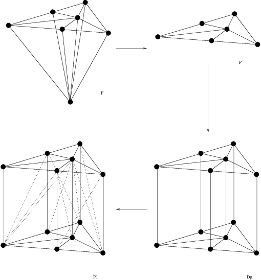
Next, we linearly map to as follows. On the upper face, we take the vertices of to the vertices of that give the pointed structure to . On the lower face of , we take the vertices to the points in Lemma 4.7 that give the pointed structure to the cycle . This defines a collection of pointed -cones in , and hence defines a chain .
From the construction, we have , where is a chain induced by the outer sides of . To finish the proof, we must show that .
To see this, let be a maximal proper face of , and let be the subset of corresponding to . By Proposition 3.16, we have . In fact, determines a unique proper rational boundary component such that .
Any 1-cone in that meets is a subset of , and hence also lies in . This means that the intersection of with the lower face of determines a collection of cones lying in .
Now consider the portion of lying in the upper face of . The 1-cones determined by this subset include the spanning rays of as before, as well some cusps used in the construction of the . By Proposition 3.8 and the restrictions placed on these cusps in Step 2 of Theorem 4.4, these cusps also lie in . Hence all the cones in the image of lie in . Applying this argument to all maximal proper faces of completes the proof.
∎
Finally we complete the proof of the theorem.
4.10.
Now we modify our algorithm to work on cycles , where . The basic construction is the same, but there is one crucial difference. When , the boundary of any automatically lies in . But for to be a relative cycle when , its boundary can meet ; this part must vanish mod . This means that we must be vigilant in our construction to ensure that the choices in Theorem 4.4 and Lemmas 4.6–4.9 can be made equivariantly over .
4.11 Theorem.
Let with . Then the choices in Theorem 4.4 can be made -equivariantly. Specifically,
- (1)
The fans can be constructed -equivariantly, yielding a fan .
- (2)
For any two 1-cones satisfying with , the corresponding cusps and can be chosen in Step 2 to satisfy .
Furthermore, the construction of from in Lemma 4.9 can be performed -equivariantly over all of . Thus, the algorithm in Theorem 4.4, with the modifications above, can be used to construct a cycle satisfying .
Proof.
The first assertion is the key, for if the fans can be constructed -equivariantly, then any construction using them can be done -equivariantly by choosing representatives for the -orbits.
Now the intersection of with consists of a finite set of simplicial cones, so a fortiori there are only a finite number of such cones modulo . This means that we may adapt the proof of Proposition 3.6 and construct the refinements using induction on the dimension. ∎
5. Second Algorithm
In this section we show how to transform cycles in to cycles in without explicitly constructing the fans from §4.1. Instead, we assume only the existence of an “oracle” that answers the following question:
Given a point , which Voronoǐ cone contains ?
This oracle for is the Voronoǐ reduction algorithm [23][12]. Since the rational boundary components are self-adjoint homogeneous cones of lower rank, and they receive a Voronoǐ decomposition by (Proposition 3.8), we are justified in assuming the existence of this oracle on both and its boundary components. Furthermore, in practice the oracle is not difficult to implement, and requires only slightly more information than that necessary for cohomology computations with .44 4 See [14] for implementation in the case of . Accordingly, we define
5.1 Definition.
Given a point , let be the set of cusps that span the unique smallest Voronoǐ cone containing . By abuse of notation, we also write for a 1-cone .
The idea behind our second algorithm is this. Although it is expensive to construct the fans , it is easy to subdivide a lift into a cycle supported on smaller pointed simplicial cones. If the top-dimensional cones in are small enough, then any two nearby 1-cones will lie in the same or adjacent cones of . Thus will be nonempty. Hence we can hope to choose cusps and assemble them into Voronoǐ cones as in Theorems 4.4 and 4.11 to build a cycle in . This is the approach we take, but our task is complicated by two issues:
- •
For efficiency, we want to subdivide as little as possible.
- •
All choices must be made -equivariantly.
To address these issues, we introduce sufficiently fine decompositions of a fan with respect to (§5.4) and the relative barycentric subdivision of a fan with respect to a subfan (§5.2). Theorem 5.12 describes an algorithm that constructs sufficiently fine decompositions, and Theorem 5.15 shows how to use such a decomposition to transform a cycle in to a cycle in in the same homology class.
5.2.
Let be the standard -simplex (§3.12), and let be the finite set . There is a bijection between faces of and subsets of : the subset corresponds to the convex hull of .
Recall that the barycentric subdivision of is the simplicial complex with vertices corresponding to nonempty subsets of , and with -faces corresponding to proper flags of length :
We denote the barycentric subdivision by . Using the concrete description of given in §3.12, we may realize the vertex of corresponding to by the point .
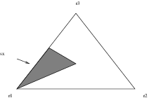
There is another approach to the barycentric subdivision using the stellar subdivision . As an abstract simplicial complex, is isomorphic to the -simplex. In the embedding of given in §3.12, is the image of the affine map that takes and is the identity on the other vertices (Figure 3). The image of is called the star point.

The barycentric subdivision can now be constructed as follows. First construct . Then stellar subdivide the original -faces of , and take the cone of these faces using the star point of as the cone point. Continue subdividing the lower-dimensional faces of the original , each time coning with the previously constructed star points. After the -faces have been subdivided, the result is (Figure 4).

Now let be a closed union of proper faces of . We define the relative barycentric subdivision as follows. We construct the sequence of stellar subdivisions above, but do not subdivide any simplices in (Figure 5).
Both the barycentric subdivision and the relative barycentric subdivision can be iterated, and we denote the resulting simplicial complexes by respectively .

Let be a pointed simplicial cone. Then the barycentric subdivision of is the fan constructed by barycentrically subdividing the simplex spanned by the tuple . We denote the 1-cone on the barycenter of by . We may similarly construct the relative barycentric subdivision of with respect to a union of proper faces. Finally, we may apply either construction to a fan of pointed simplicial cones by applying it to each simplex separately.
5.3 Remark.
Elementary arguments show that the set of vertices in becomes dense in as , no matter what proper subcomplex we choose.
5.4.
We want to formalize how much a given fan must be subdivided for our purposes. Recall that denotes the set of spanning rays of a cone , and that if is a 1-cone, then denotes the set of spanning rays of the unique smallest Voronoǐ cone containing .
5.5 Definition.
Let be a -dimensional simplicial cone, and let be a finite simplicial fan with . Then the fan is said to be a sufficiently fine decomposition of if the following is true: for every -cone , we have
| (3) |
More generally, we can speak of a sufficiently fine decomposition of a set of -cones. In this case, we mean that each cone in the set has been refined into a fan whose -cones satisfy (3).
5.6 Example.
Suppose that is a -cone, i.e. is a cone on an interval . Then a partition of into intervals induces a sufficiently fine decomposition of if and lie in adjacent or the same Voronoǐ cones. (The condition on barycenters is automatic in this case.) This is equivalent to the notion of sufficiently fine for modular symbols for -rank one groups presented in [12].
5.7.
We want to discuss the relationship between sufficiently fine decompositions and the canonical fans of §4.1. We begin by introducing an open covering of a fan.
5.8 Definition.
Let be a fan. Given any , let be the open star of in . In other words,
Let be .
Notice that if , then . Also, if is a subfan (a subset of that is also a fan), then
In general the sets in are not convex, although they are star-shaped.
Let be the canonical fan , with no simplicial refinement.
5.9 Proposition.
Let be a simplicial -cone, and let be a simplicial fan that is a refinement of . Let , and let be the barycenter of . Then satisfies (3) if and only if there is a set such that .
Proof.
Assume satisfies (3). Then there is a Voronoǐ cone such that . This Voronoǐ cone induces . The open star of in the canonical fan is the intersection of with the open star of in . Then is contained in . The converse is obtained by simply reversing this argument.
∎
A consequence of the preceding Proposition is that sufficiently fine decompositions exist for any rational simplicial cone in .
5.10 Proposition.
Let be a rational simplicial -cone. Then the fan gives a sufficiently fine decomposition of for .
Proof.
By Proposition 5.9, any fan subordinate to gives a sufficiently fine decomposition of . Hence the statement follows immediately from the fact that is finite. ∎
5.11.
We now describe an algorithm that constructs sufficiently fine decompositions of a given set of cones. Recall that if is a set of cones, the we let .
5.12 Theorem.
Let , and let . Then the following algorithm constructs a sufficiently fine decomposition of :
- (1)
Set , and set .
- (2)
Assume that has been constructed for , where . Let be any -equivariant extension of to without adding new 1-cones (see Figure 6). Then for some , the fan given by the relative barycentric subdivision is sufficiently fine, and can be taken for .
- (3)
If , terminate. Otherwise, increment and return to Step 2.

Proof.
We must verify two facts. First we claim that can be constructed -equivariantly. This follows because each of the sets is finite modulo , and so we may subdivide a set of representatives and translate by , as in Proposition 3.6.
Now we claim that will be sufficiently fine for . If we were performing the usual barycentric subdivision, then by Proposition 5.10 we would succeed. We must show using the relative barycentric subdivision with respect to poses no obstruction.
So let be a -cone that appears in the refinement of a given . Let be the barycenter of . Since is sufficiently fine, Proposition 5.9 implies that there exists a set , the open star , such that
(See Figure 7. In this and the following figure, we depict a generic affine slice of these objects.)

Suppose that appears as a face of a simplex . Then the canonical fan is a subfan of , which implies . Moreover, is the intersection of with the set . We can picture as a “thickening” of into .
Now extend to , and begin iterating the relative barycentric subdivision. Away from , the new -cones will fill densely, and by Proposition 5.10 the decomposition will become sufficiently fine there. The only possible problem is near . Over each , the new -cones of will converge to . In Figure 8 we show the affine slices of these -cones as grey dots. By Remark 5.3, these new -cones come arbitrarily close to and eventually enter . By Proposition 5.9, this implies will be sufficiently fine for some .

∎
5.14.
We conclude the paper by showing how a sufficiently fine decomposition as in Theorem 5.12 may be used to transform a cycle in to a cycle in giving the same homology class in .
5.15 Theorem.
Let be a Hecke image, and let be a -equivariant sufficiently fine decomposition of . Let be the barycentric subdivision of . Then the following algorithm constructs a cycle satisfying .
- (1)
Each 1-cone is the barycenter of a set of -cones of . For each , choose a cusp . Make these choices -equivariantly over . Let be the vertex of generating .
- (2)
Each -cone corresponds to a flag
where each is a -cone in (cf. Figure 9). For each such flag, assemble the points
into a -tuple , using the orientation on . Form rational pointed cones using these tuples.
Then the desired cycle is
Proof.
Let be a set indexing a -cone . Then the definition of sufficiently fine implies that the set is nonempty. Hence we may select a cusp . Also, the cusps can be chosen -equivariantly over all of by applying a neatness argument similar to Proposition 3.6.
Next, that is homologous to follows from arguments identical to those presented in Lemmas 4.7 and 4.9.
What remains to be shown is that the cones are Voronoǐ cones. This follows since the cusps
are all spanning rays of the Voronoǐ cone containing . (See Figure 10 for an example when and .) Since this Voronoǐ cone is simplicial, this completes the proof of the theorem. ∎

References
- [1] A. Ash, Deformation retracts with lowest possible dimension of arithmetic quotients of self-adjoint homogeneous cones, Math. Ann. 225 (1977), 69–76.
- [2] by same author, Galois representations and cohomology of , Séminaire de Théorie des Nombres, Paris, 1989–90, Progr. Math., vol. 102, Birkhäuser Boston, Boston, MA, 1992, pp. 9–22.
- [3] by same author, Unstable cohomology of , J. Algebra 167 (1994), no. 2, 330–342.
- [4] A. Ash and M. McConnell, Experimental indications of three-dimensional galois representations from the cohomology of , Experiment. Math. 1 (1992), no. 3, 209–223.
- [5] A. Ash, D. Mumford, M. Rapaport, and Y. Tai., Smooth compactifications of locally symmetric varieties, Math. Sci. Press, Brookline, Mass., 1975.
- [6] A. Ash, R. Pinch, and R. Taylor, An extension of attached to a non-selfdual automorphic form on , Math. Ann. 291 (1991), 753–766.
- [7] A. Ash and L. Rudolph, The modular symbol and continued fractions in higher dimensions, Invent. Math. 55 (1979), 241–250.
- [8] A. Borel and J.-P. Serre, Corners and arithmetic groups, Comm. Math. Helv. 48 (1973), 436–491.
- [9] J. E. Cremona, Hyperbolic tessellations, modular symbols, and elliptic curves over complex quadratic fields, Compositio Math. 51 (1984), no. 3, 275–324.
- [10] J. Faraut and A. Korányi, Analysis on symmetric cones, Oxford Mathematical Monographs, Oxford University Press, New York, 1994, Oxford Science Publications.
- [11] F. Grunewald and J. Schwermer, A nonvanishing theorem for the cuspidal cohomology of over imaginary quadratic integers, Math. Ann. 258 (1981), 183–200.
- [12] P. Gunnells, Modular symbols for -rank one groups and Voronoǐ reduction, to appear, 1997.
- [13] by same author, Symplectic modular symbols, submitted, 1997.
- [14] D.-O. Jaquet, Domaines de Voronoi et algorithme de reduction des formes quadratiques definies positives, Sem. Theor. Nombres Bordeaux (2) 2 (1990), no. 1, 163–215.
- [15] A. Krieg, Hecke algebras, Mem. Amer. Math. Soc. 87 (1990), no. 435, x+158.
- [16] R. Lee and R. H. Szczarba, On the homology and cohomology of congruence subgroups, Invent. Math. 33 (1976), no. 1, 15–53.
- [17] I. Satake, On representations and compactifications of symmetric Riemannian spaces, Ann. Math. 71 (1960), 77–110.
- [18] by same author, On compactifications of the quotient spaces for arithmetically defined discontinuous groups, Ann. Math. 72 (1960), 555–580.
- [19] G. Shimura, Introduction to the arithmetic theory of automorphic forms, Princeton University Press, 1971.
- [20] R. Taylor, -adic representations associated to modular forms over imaginary quadratic fields. II, Invent. Math. 116 (1994), no. 1-3, 619–643.
- [21] J. Tits, Tabellen zu den einfachen Lie Gruppen und ihren Darstellungen, Lecture Notes in Mathematics, vol. 40, Springer-Verlag, 1967.
- [22] B. van Geemen and J. Top, A non-selfdual automorphic representation of and a Galois representation, Invent. Math. 117 (1994), no. 3, 391–401.
- [23] G. Voronoǐ, Sur quelques propriétés des formes quadratiques positives parfaites, J. Reine Angew. Math. 133 (1908), 97–178.
- [24] S. Zucker, Satake compactifications, Comment. Math. Helvetici 58 (1983), 312–3439.