The Dodecahedral Conjecture
Abstract
This article gives a proof of Fejes Tóth’s Dodecahedral conjecture: the volume of a Voronoi polyhedron in a three-dimensional packing of balls of unit radius is at least the volume of a regular dodecahedron of unit inradius.
1 Introduction

A packing of congruent unit radius balls in three-dimensional Euclidean space is determined by and is identified with the set of centers of the balls. A packing determines a region called the Voronoi cell around each ball. The Voronoi cell around a ball at consists of points of space that are closer to than to any other . The Voronoi cell is a convex polyhedron containing . Figure 1 shows the Voronoi cells of a finite packing.
The Dodecahedral conjecture asserts that in any packing of congruent balls of Euclidean space every Voronoi cell has volume at least that of a regular dodecahedron of inradius (Figure 2). This bound is realized by a finite packing (of twelve balls and a thirteenth at the origin) obtained by placing a point of at the center of each face of a regular dodecahedron (of inradius ).
The assertion can then be stated as the inequality
for every , and for every set of points whose pairwise distances are at least the diameter . The case of equality occurs exactly when is congruent to a regular dodecahedron of inradius .
1.1 History
L. Fejes Tóth made the conjecture in 1943 [34]. In that article, L. Fejes Tóth sketches a proof based on an unproved hypothesis. This hypothesis is a quantitative version of the kissing number problem in three dimensions. This unproved hypothesis is now generally regarded as being nearly as difficult as the Dodecahedral conjecture itself.
L. Fejes Tóth returned to the Dodecahedral conjecture in a number of publications. It is a prominent part of his two books [36], [35]. According to the strategy of [36], the Dodecahedral conjecture forms a step towards the solution of the sphere packing problem (discussed below). In [35] , he proved that the Dodecahedral conjecture holds for every Voronoi cell with at most twelve faces. This result is reviewed in Section 4. It is an ingredient in the proof presented here.
A lower bound on the volume of a Voronoi cell implies an upper bounds on the density of packings of congruent balls in three dimensions. The Dodecahedral conjecture gives an upper bound on density of . Upper bounds on the density based on lower bounds on the volume of a Voronoi cell in the literature include Rogers’ upper bound 0.7797 [33], and Muder’s upper bounds 0.77836 [27] and 0.7731 [28].
In 1993, Hsiang published what he claimed to be proofs of the Kepler conjecture and the Dodecahedral conjecture [22]. However, the proof did not hold up to careful analysis. “As of this writing, Kepler’s conjecture as well as the dodecahedral conjecture are still unproven” [4, p761]. See also, [12].
An alternative approach to the Dodecahedral conjecture is described in [4]. Unfortunately, a counterexample has been found to both parts of the third conjecture of that article. The counterexample is described in the preprint [16]
K. Bezdek conjectures that the surface area of any Voronoi cell in a packing of unit balls is at least that of a regular dodecahedron of inradius . This strengthened version of the Dodecahedral problem is still open [5].
1.2 The sphere packing problem
The Kepler conjecture, also known as the sphere packing problem, asserts that no packing of congruent balls in three dimensions has density greater than the density of the face-centered cubic packing. S. McLaughlin carried out the research for the proof of the Dodecahedral conjecture at the University of Michigan while S. Ferguson and T. Hales worked on the sphere packing problem. Both problems were solved in 1998.
There is no strict logical connection between the two problems. The Dodecahedral conjecture does not follow from the Kepler conjecture and is not an intermediate step in the solution to the Kepler conjecture. (In Fejes Tóth’s strategy, it was an intermediate step; however, that strategy was not followed in the solution of the sphere packing problem.) Nevertheless, the two solutions follow a similar outline and share a significant number of methods. Both are based on long computer calculations. Computer code was freely exchanged between the two projects.
This article is written in a way that it is not necessary to read or understand the solution of the sphere packing problem before reading this article. However, for the benefit of the reader, this article points out parallels with the sphere packing problem. It also cites various results from that proof.
1.3 Differences
Although the proof of the Dodecahedral conjecture runs parallel to the solution to the sphere packing problem, there are special difficulties that arise in the proof of the Dodecahedral conjecture. In no sense is it a corollary of the sphere packing problem. In the packing problem, there turn out to be many ways to reduce the infinite ball problem to a problem about finite clusters of balls. This multiplicity of choices makes it possible to design many difficulties away. If one reduction is not satisfactory one can work with another. With the Dodecahedral problem, there is no such flexibility. The problem about finite clusters of balls is fixed from the outset. This gives the problem a degree of rigidity that is not present in the sphere packing problem.
1.4 Ten years later
Over ten years have elapsed from the completion of the research until publication. A few words of explanation are in order. The review and publication process for the Kepler conjecture extended from 1998 until 2006. Because of significant sharing between the Kepler conjecture and the Dodecahedral conjecture, a “wait and see” attitude developed toward the Dodecahedral conjecture. Once the Kepler conjecture was published, the path became clear for the publication of Dodecahedral conjecture.
The details of the proof in the current publication are essentially the same as those in the preprint posted on the arXiv [17] in 1998. No significant errors have emerged in the original 1998 preprint. However, the article has undergone various major rewrites since then, including a significantly expanded version in 2002 [16]. That version is written in such a way that it is entirely independent of the proof of the Kepler conjecture. As an abridgment of a longer version, this article replaces some proofs with summaries and references. This article refers the reader when necessary to relevant passages in the full version of the proof. The computer code has also been entirely rewritten.
A formalization project, called Flyspeck, aims to provide a complete formalization of the proof of the Kepler conjecture [15, 11]. (A formal proof is one in which every logical inference of the proof has been independently checked by computer, all the way to the primitive axioms at the foundations of mathematics.) A parallel project, called Flyspeck Light, aims to do the same for the proof of the Dodecahedral conjecture. These long-term projects will take many years to complete. Nevertheless, significant progress has already been made toward the formal verification of the computer code [29, 30]. The revisions in this article incorporate the parts of Flyspeck Light that have already been completed.
1.5 Truncation
The distance from the center of the regular dodecahedron to a vertex is . This parameter is used to truncate Voronoi cells; it makes volumes easier to estimate. A similar truncation takes place in the solution to the packing problem with truncation parameter . It is a happy coincidence that these two truncation parameters are so close to one another. A great deal of duplicated effort might have been avoided if these two parameters were equal. However, the parameter cannot be replaced with anything smaller, and although the parameter could easily have been made larger, its value was already too deeply entrenched in published articles by the time work started on the Dodecahedral conjecture.
As a first step towards unifying the proofs, many results can be stated in a form that holds for all . To transfer a lemma from [18] to this article, a simple process is involved. The first step is generalization, replacing the constant with a free parameter . The second is specialization, .
The number , although rational, can be consistently treated as an independent real transcendental in the solution to the sphere packing problem; that is, none of the proofs involving rely on its exact numerical value. The constant can always be replaced by a constant in a suitably small interval about . However, the only way to know that this small interval is wide enough to contain is to study the details of the proof. We have made a detailed study of relevant proofs in [18] to insure that they can be adapted to the present situation.
As a matter of terminology, a proposition for the Dodecahedral conjecture is said to be a reparametrization of a proposition with the constant , if it is obtained by mechanically replacing with , wherever that constant appears, and if the proof goes through verbatim with this minor change. When this occurs, there is nothing to further to be learned by repeating the proof. The cited proposition already contains all the needed detail.
1.6 Terminology
Various notation and terminology is shared between the solution of the sphere packing problem and this article. Vocabulary can be imported from the sphere packing problem three different ways. The simplest way to import a term is for the term to have precisely the same meaning in both places. For example, the terms “orientation” and “packing” have the same meaning in both places.
The second way to import a term is by making a reparametrization of a term that depends on the parameter . For example, the definition of standard component in this paper is the reparametrization of standard component in [18].
The third way in which terms have been imported into this proof from the proof of the Kepler conjecture has been by structural analogy. For example, the term tame graph is a technical notion that arises in the solution of the sphere packing problems. At the analogous point in this proof, a somewhat related collection of graphs appears. To emphasize the analogous role they play in the proof of the Dodecahedral conjecture, they are called tame Voronoi graphs. Similarly, there is a strong analogy between Voronoi weight assignments in this article, and admissible weight assignments in [18].
There are a some terms in that have been renamed in this version for greater precision. Special has become unstable, standard region has become standard component, dihedral angle has become azimuth angle, and non-external has become internal. Planar maps have been replaced with hypermaps. A few terms (such as distinguished) have been slightly redefined, when doing so is harmless.
2 Outline
This section gives a precise statement of the main theorem and describes the broad outline of the proof.
2.1 Formulation
This article proves the Dodecahedral conjecture in a stronger version than that stated in the abstract. A truncation of the Voronoi cell already has volume at least as great as that of the regular dodecahedron. This subsection describes the truncation and states the stronger version of the main theorem in a precise form.
Let be a packing and let . Let be a closed ball of radius centered at . Let . Let be the set of all consisting of four distinct points such that for all and such that the circumradius of each triangle is at most . Write for the convex hull of .
Define the following truncation of the Voronoi cell :
That is, the the Voronoi cell is truncated by intersecting it with a ball of radius , except inside regions protected by the sets . Note that the special packing satisfies . The Dodecahedral conjecture takes the following strengthened form.
Theorem 2.1.
For every packing and every ,
Equality holds exactly when is congruent to .
2.2 Proof outline
The Lebesgue measure is translation invariant. Thus it does no harm to assume that the center point of the Voronoi cell lies at the origin: . The assumption that remains in force for the rest of this article.
The next reduction is to replace the set with . This is accomplished by the following lemma, which shows that the volumes in Theorem 2.1 are insensitive to points of outside . The proof appears in Lemma 5.3.6.
Lemma 2.2.1.
Let be any packing (with ). Then
The condition is a standing assumption for the rest of the article. Let and let be the cardinality. The proof of Theorem 2.1 splits into two main cases: and . In fact, L. Fejes Tóth settles the case in his book [35]. Section 4 sketches Fejes Tóth’s proof.
Completely different methods treat the case when . This part of the proof is considerably more difficult than the case treated by Fejes Tóth. Here is a sketch of the proof of the case . This rough sketch will be expanded in greater detail later in the article.
Let be a packing satisfying the standing assumptions that and . The Dodecahedral conjecture seeks a minimum to the objective function
This is a nonlinear optimization problem in finitely many variables. The target value for the minimization is . When , this article proves11 1 An examination of the proof shows the right-hand side can be improved to . In fact, in terms of notation to be described later in the article, the proof only relies on the bound for triangles , but in fact every configuration has at least one triangle with ,
Some combinatorial information about each packing is encoded as a graph. The vertex set of the graph is . (Because of this graph, elements of are generally called vertices.) The edge set is
This is a planar graph. The Dodecahedral conjecture reduces to the case when this graph is connected. In fact, when the graph is not connected, this article constructs another packing whose graph is connected, with the same cardinality as , and such that
Similarly, the conjecture reduces to the case where the graph is biconnected. This again involves constructing an auxiliary packing of the same cardinality and whose truncated Voronoi cell has the same volume. Now assume that the graph of is biconnected.

This article supposes the existence of a counterexample to the Dodecahedral conjecture and makes a detailed study of the properties of its graph. It defines a class of graphs (called tame Voronoi) and proves that the graph of every counterexample is tame Voronoi.
Tame Voronoi graphs can be described in purely combinatorial terms, without reference to packings, Voronoi cells, and volumes. All tame Voronoi graphs can be classified up to isomorphism. This classification is one of the main steps of the proof. There are only finitely many possibilities. Thus, the graph of any counterexample to the Dodecahedral conjecture must be one of these finitely many cases.
Each tame Voronoi graph can be encoded as a hypermap . (A hypermap can be defined as a finite set, together with two permutations on that set. The elements of the given finite set are called darts.) If is a hypermap, let be the finite dimensional vector space of real-valued functions on its set of darts. The pair is called a hypermap system if is a set of boolean valued functions for some . A hypermap system is feasible if there is some such that holds for all . The computer code repository specifies a hypermap system, called the Voronoi hypermap system, for each case arising in the classification of tame Voronoi graphs.
Another major step of the proof is the proof that every Voronoi hypermap system is infeasible (Theorem 8.1). The proof of this theorem is a case-by-case analysis based on the explicit enumeration of tame Voronoi graphs, up to isomorphism. The feasibility problem for each Voronoi hypermap system is converted to a system of linear programs. The infeasibility of the Voronoi hypermap system follows from the infeasibility of the corresponding linear program.
If there exists a counterexample to the Dodecahedral conjecture, there is an associated Voronoi hypermap system . By the preceding result, this hypermap system is infeasible. On the other hand, the counterexample can be used to construct a feasible solution to the system (Theorem 8.2). This contradiction shows that a counterexample cannot exist. In this way, the Dodecahedral conjecture is proved.
3 Computation
The proof of the Dodecahedral conjecture is based on a series of computer calculations. This section briefly describes the computer algorithms, the code implementing those algorithms, and issues of the reliability of the computer code.
There are three main computer programs that are used in the proof. The first is a graph generator that generates, up to isomorphism, all planar graphs satisfying a list of properties. The second is a linear programming package. The third is a piece of code based on interval arithmetic that automatically proves nonlinear inequalities over the real numbers. This section discusses each in turn.
This section also discusses some additional computer programs. Although these computer programs, strictly speaking, are not part of the proof, they are relevant to understanding the structure of the proof and the reliability of the computer implementation. We include a brief discussion of nonlinear optimization software, Tarski’s decision procedure for real-closed fields, and formal theorem proving packages.
3.1 Electronic resources
A permanent archive has been set up for all of the external resources related to this proof [26]. This archive is under version control by Google Code [10]. The site consists of a download area where one may obtain the source code and supporting documents to this paper. Additionally there is a subversion [8] repository. This means that the snapshot of the code and documents in the exact form they took at the time of creation is permanently available. It also means that any changes (for instance, a bug fix) will leave a permanent public electronic trail. The major components of [26] are:
- 1.
The source code for the three different programs used in the proof (graph generation, linear programs, and interval arithmetic inequality prover)
- 2.
A list of all tame Voronoi graphs, up to isomorphism.
- 3.
A list of inequalities that have been established by interval arithmetic.
- 4.
A list of the inequalities that have been used in linear programming.
Additional information, such as source code documentation, is available as well.
3.2 Tarski arithmetic
The Dodecahedral conjecture, after a few preliminary reductions, can be expressed as a statement in the elementary language of the real numbers. The elementary language of real numbers is a first order language built from quantifiers (), logical connectives (), functions symbols for ring operations (), variables , and constant symbols (). By a fundamental result of Tarski, the elementary theory of the real numbers is decidable. Thus, the truth of the Dodecahedral conjecture can be decided in theory by standard algorithms such as Collin’s cylindrical algebraic decomposition [7], or the Cohen-Hörmander algorithm [21]. However, in practice, these decision procedures take exponential time in the number of quantifiers, and thus are far too slow to be of practical value for this conjecture.
To formulate the Dodecahedral conjecture as a statement in the elementary theory of the reals, consider Voronoi cells without truncation, centered at the origin. The volume of the regular dodecahedron is an algebraic number , hence definable in Tarski arithmetic. Also, there are a priori bounds on the number of faces of the Voronoi cell, and thus also on the size of the clusters of balls that give candidates for counterexamples. For example, by adding balls to the packing to decrease the volume, the packing becomes saturated. Assuming saturation, E. Harshbarger gives a quick calculation of faces [19]. (The exact value of this constant is not important as long as it is explicitly given.) The assertion of the Dodecahedral conjecture is then expressed as an enormous conjunction of cases, with conjuncts indexed by an explicit enumeration of all possible combinatorial structures of a Voronoi cell, including a fixed triangulation of each face of the cell. The fixed triangulation determines a partition of the Voronoi cell into tetrahedra. The volume of each tetrahedron is expressed by means of a Cayley-Menger determinant as a definable function of the the edge lengths of the tetrahedron. Thus, for each combinatorial structure with faces, a Tarski statement asserts that for all vectors , if the Voronoi cell defined by the vectors has combinatorial structure , then the volume of the cell is at least . The outer block of universal quantifiers – not to mention the nested existential quantifiers – is hopelessly beyond the practical reach of current algorithms. The statement that the regular dodecahedron is the unique minimizer can be similarly expressed.
If the entire Dodecahedral conjecture can be expressed in Tarski arithmetic, then perhaps it is not so surprising that many of the intermediate steps in the proof can also be so expressed. These intermediate steps also tend to be beyond the reach of current decision procedures. But here the situation is not so hopeless. Many of these intermediate problems involve no more than a dozen quantifiers. One can imagine the day that these problems might fall within the reach of decision procedures for Tarski arithmetic.
Describing various intermediate steps of the proof as exercises in Tarski arithmetic is a useful point of view. Doing so identifies a family of subproblems that can be expressed in a common language, and that can often be solved by similar techniques. The complexity of the problems can be measured objectively by counting the number quantifiers.
Here are some geometrical objects that are definable within the Tarski arithmetic that appear in the proof of the Dodecahedral conjecture. By Heron’s formula, the circumradius of a triangle with sides is elementary definable. Set
for three points . The volume of a tetrahedron with vertices is elementary definable. In fact, by Cayley-Menger determinants, there is a polynomial of the six squared edge lengths such that
In particular, , whenever the variables have the form for some points [13, Lemma 8.1.4].
The orientation of in is said to be positive (zero, negative) when and the circumcenter of lie on the same side of (resp. on, on opposites side of) the plane passing through [18, Lemma 5.15]. This is an elementary condition.
For , let be the cone with apex generated by :
Write for the corresponding set with strict inequality . Let be the convex hull
Write when the inequality is strict .
Define the right circular cone by the formula
For a set of fixed finite cardinality, the membership conditions , , can be expressed in the Tarski language.
In preparing this abridged version, the proofs of numerous statements in the Tarski language (involving a small number of quantifiers) have been omitted. These tend to be the arguments that can most easily be skipped without disrupting the overall flow of the proof. The full proofs appear at [16].
3.3 Formal proof
A formal proof is a proof in which every logical inference has been checked, back to the foundational axioms of mathematics. Except in trivial cases, a computer is used to generate a formal proof, because of the large number of inferences involved. Both conventional proofs and computer assisted proofs can be formalized. In a computer assisted proof, this amounts to a formal verification of the correctness of the computer code. Formal verification of computer code is a difficult task. For that reason, formal verification tends to be reserved for situations where correct performance is critically important, such as the verification of aircraft control systems, cryptography algorithms, and security protocols for the internet. There is no other means of checking computer software that can assure reliability at levels that remotely compare with the assurance afforded by formal verification.
There is a long term project, called Flyspeck Light, to give a formal verification of the Dodecahedral conjecture. Although this project is far from complete, parts of this project have already been carried out. This means that some of the computer code for this project now carries a proof of correctness, according to formal mathematical standards. One such program is discussed in the next subsection.
3.4 Graph generation
The proof of the Dodecahedral conjecture is based on three separate computer programs. The first of these is a planar graph generator. It generates all planar graphs, up to isomorphism, that satisfy a given list of restrictions. The restrictions include a bound on the number of vertices in the graph, so that it is obvious that only finitely many graphs are possible.
The correctness of the graph generator program has been the subject of extensive mathematical investigation. Early versions of the program were written by Hales in 1994 (in Mathematica), 1997 (in Java), and 2000 (in Java). The same computer program is used in the Kepler conjecture and Dodecahedral conjecture. They differ only in their input parameters. This computer program became the subject of G. Bauer’s dissertation in computer science at the Technical University of Munich [2]. This 172-page dissertation translates the Java code into the formal theorem proving system Isabelle/HOL [31] and gives a detailed mathematical treatment of the graph theory underpinning the computer code. The dissertation analyzes every line of code. Building on the work of this thesis, B. Bauer and T. Nipkow have completed the formal correctness proof of the HOL implementation of the graph generator [29]. (Their published article mentions only the Kepler conjecture, but the formal verification has been extended to apply to the input parameters of the Dodecahedral conjecture as well.) As a result of this work, the graph generation is currently the most scrupulously checked part of the proof of the Dodecahedral conjecture.
There are several published sources that provide details of this algorithm, and there is no need to repeat details here. The basic idea is to start with a small set of planar graphs (called ‘seed’ graphs) with the property that every planar graph to be classified is known to have one of the seed graphs as a subgraph. The seed graphs are then extended by adding one face at a time. Faces are added in all possible ways so that it is clear at every step of the algorithm that every biconnected planar graph will be generated. At the same time, pruning operations discard partially completed graphs when it can be shown that the partial graph is not a subgraph of any of the graphs to be classified. The pruning operations prevent a combinatorial explosion of cases. See [14, §5], [18, §19], [2], [29].
3.5 Linear programs
The second computer program that is used in the proof of the Dodecahedral conjecture is linear programming. There are several hundred linear programs that appear in the proof.
Formal verification has not yet been extended to this portion of the computer code. However, the recent dissertation of S. Obua takes the first steps in this direction [30]. That work gives a formal correctness proof of the basic linear programs that appear in the proof of the Kepler conjecture. In particular, he has developed all the infrastructure needed to carry out formal correctness proofs of linear programming problems. The formalization completed by Obua is a larger project than the formalization of the linear programming segment of the Dodecahedral conjecture. Thus, one can expect that the formalization of this piece of computer code will soon follow suit.
In the 1998 proof, computer code written in C generated the linear programs, which were then fed to the commercial linear programming package CPLEX. In preparation for a formal proof, the computer code has been rewritten in the programming language Standard ML (SML), with an external interface to the solver GLPK.
It is not necessary to trust the algorithms of the linear programming packages (such as CPLEX and GLPK) that solve the linear programs. These packages produce dual certificates that can be used to give independent verification of the solutions of the linear programming problems.
In the proof of the Dodecahedral conjecture, the following situation arises. The objective is to prove that the maximum of a linear function is less than a given constant , when subject to a system of linear constraints . Here , , are vectors with real entries and is a matrix with real entries. The products are given by matrix multiplication of compatibly sized matrices and vectors. A vector inequality means that for each coordinate . Explicit lower and upper bounds on the variables are given: . Expressed equivalently, the objective is to show that the linear system of inequalities
has no solutions in . The external linear programming package produces a dual certificate in the form of a vector , which that package claims to have the properties
| (1) |
If indeed has these properties, then for any satisfying , it follows that
| (2) |
as desired.
Because of inexact arithmetic used by the external packages, these identities will only be approximately correct. The imprecision in the dual certificate can be readily eliminated as follows. If is any vector, let be the vector obtained by replacing the negative entries of with , and let be the vector obtained by replacing the positive entries of with . By replacing the vector with , the vector satisfies . In the following lemma, and are small error terms that result from machine approximation. By including them in the bounds on , a rigorous bound can be recovered.
Lemma 3.5.1.
Suppose that the real-valued vectors and matrices , , , satisfy the following relations
Define residuals
If
then .
Proof.
The numerical data are all explicitly given, so that the method yields explicit bounds. It is not necessary to trust the package that produces the certificate , because all of the assumptions of the lemma can be checked directly with simple matrix multiplications. The reliability of these matrix multiplications is guaranteed by using interval arithmetic.
3.6 Interval arithmetic
The third major computer program that is used in the proof of the Dodecahedral conjecture is an nonlinear-inequality prover over the real numbers based on interval arithmetic. This subsection describes the methods involved and the computer implementation.
A finite number of nonlinear functions are given. It is assumed that all functions have the same domain
given as a product of intervals in , for some . The computer program verifies that
| (3) |
for every point . The approach is similar to the approach described in R. B. Kearfott [24], based on interval arithmetic. Our methods are similar to algorithms in widespread use for rigorous global optimization. Closely related algorithms are also described in [37].
The method is based on an iteratively refined partition of the domain into a finite number of smaller and smaller rectangles that cover .
Start with , then repeat the following procedure. Pick ; replace with ; and calculate a lower bound , for all . If for some , then the desired bound (3) holds on . If the desired bound holds on , then continue to the next rectangle in . Otherwise, choose finitely many rectangles, that cover ; replace with , then repeat. The procedure terminates when . (If the procedure is applied to a false disjunction (3), there is no termination.)
When subdividing rectangles to obtain smaller covers, one does it in such a way the the width of the rectangle tends to zero as iteration continues. In this way, the lower approximations to can be arranged to converge to the true minimum of on the rectangle.
The lower bounds to a function on a rectangle are obtained by methods of interval arithmetic. The function is generally on its domain.22 2 The functions encountered in practice are usually , but not always so. When functions are not , Taylor approximations are avoided. The function can be expanded in a Taylor polynomial approximation with explicit error bounds. Derivatives are calculated by automatic differentiation. The error bounds are based on the Lagrange form of the error term in the Taylor approximation. Interval arithmetic produces rigorous bounds on the error terms.
There have been several separate implementations of the interval arithmetic package. The source code for all of these packages is publicly available. (The code that is used for the proof of the Kepler conjecture is the same as the code that is used for the proof of the Dodecahedral conjecture. Only the statements of the inequalities to be proved differ.) The first version, written in C++, was developed by T. Hales over the period 1994-1998. A second version, written in C, was developed by S. Ferguson 1995-1997. A third version, written in SML, was developed by S. McLaughlin 2006-2008. A interval arithmetic package has also been developed by R. Zumkeller for the theorem proving system Coq [3], although it has not been used to give a formal verification of any of the inequalities that arise in the proof of the Dodecahedral conjecture [38]. These implementations are all independent of one another. (Algorithms were shared among us, but the code was independently implemented.) By comparing the proofs of different inequalities in different systems, we have developed a high degree of confidence that the implementations of the algorithms are essentially correct. Of course, it would be desirable to have a formal correctness proof, but this part of the Flyspeck Light project has not been completed. (The SML implementation and Zumkeller’s research are partial steps in this direction.)
The list of nonlinear inequalities that are used in the proof of the Dodecahedral conjecture appears at [26]. The domains of the functions are subsets of , for . The complexity of the verification increases rapidly with . This proof implements some of the tricks introduced in [18] to reduce the dimension of the domain wherever possible. Dimension reduction is based on established monotonicity properties of the functions. (For example, the volume of a Voronoi cell does not increase when it is intersected with a half-space.) Whenever the functions are twice continuously differentiable, a first order Taylor polynomial with explicit error bounds on the second derivatives is used.
The functions represent elementary geometric quantities such as linear combinations of angles, dihedral angles, solid angles, and volumes. Explicit formulas for these functions are known involving rational functions, the square root, and functions. The typical form of a function is a linear combination of terms of the form
where are explicit polynomials on . In the formula (3), the number of disjuncts is usually one , but in some cases there are two disjuncts.
The computer calculations use interval arithmetic to control for floating-point rounding errors. Every real number is represented on the computer as an interval containing , where and are exactly representable floating point numbers [1, 32]. The calculations conform to IEEE-754 standards [23]. Approximations to inverse trigonometric functions are based on published approximations [20].
3.7 Nonlinear optimization
Previous subsections describe the three main pieces of computer code used in the proof of the Dodecahedral conjecture: graph generation, linear programming, and interval-arithmetic inequality proving. This subsection describes one additional software package indirectly involved in the proof: nonlinear-optimization.
The disjunction of inequalities in formula (3) can be represented as a constrained minimization problem: show that the global minimum of on the domain
is positive.
Nonlinear optimization libraries have been used to test all the inequalities in the collection [25], [6]. The code generates a large random set of points in the domain and runs the algorithm for each initial point to find a local minimum to the objective function . If is sufficiently large and sufficiently random, it can be expected that one of the local minima produced to be a numerical approximation of the global minimum.
In practice, this approach works remarkably well on this collection of problems, largely because the functions tend to be rather bland from the point of view of nonlinear optimization. (Typically, the second derivatives of are small; the level surfaces of are approximately planar; there are no local minima in the interior of the domain; the global minimum occurs at a corner of the domain; and every run of the algorithm produces the same local minimum.) Thus, the method can usually determine the true global minimum with high probability.
If this nonlinear optimization is not part of the proof tree, what purpose does it serve? First of all, although we have tried to be careful to avoid any errors in the computer code, an independent check of the results is certainly welcome. It makes the proof more robust against possible errors. In fact, this independent check has helped us to spot and correct data entry errors. Secondly, the package was used to discover inequalities that were likely to be true, and to discard quickly inequalities that were false. The plausibly true inequalities then became candidates for rigorous nonlinear optimization with interval arithmetic.
3.8 Summary
This section has described various computer programs and algorithms that have been used in the proof of the Dodecahedral conjecture. The rest of the article assumes that the types of computations described in this section can be reliably performed by computer.
Recall briefly how the three main computer programs enter into the proof. A planar graph is associated with each potential counterexample of the Dodecahedral conjecture. The properties of this graph is studied, and it is shown to be a tame Voronoi graph. Using the graph generator program, all such graphs are classified up to isomorphism. This reduces the proof to a finite enumeration of cases. Linear programs are then used to show that each case in this enumeration is infeasible. The nonlinear inequalities appear in several different parts of the proof. They are used, for example to establish that the graph associated with a counterexample is a tame Voronoi graph. Nonlinear inequalities are also used to justify the list of inequalities used in the linear programs. (The linear programming inequalities come as linear relaxations of nonlinear inequalities.)
4 Fejes Tóth’s Reduction
L. Fejes Tóth proved the Dodecahedral conjecture under the extra hypothesis that has at most elements. The proof occupies about eight pages of the book Regular Figures [35]. See the main theorem of Section 33 and the main theorem of Section 41 (including the note on page 265). Fejes Tóth’s bound is a general bound about the volume of truncated polyhedra. The polyhedra do not need to be Voronoi cells in a sphere packing. Here is a sketch of his proof.
Theorem 4.1.
Let be any polyhedron with at most faces that contains a unit sphere . Let be the ball of radius concentric with . The volume of the intersection of with is at least . Equality holds exactly is congruent to the regular dodecahedron .
Proof.
(Sketch) By translation, the proof reduces to the case that the origin is the center of . If , there is a polyhedron with smaller volume and faces, obtained by clipping a corner of the polyhedron with a new face. Thus, assume . View the case in which some vertices of the polyhedron have degree greater than as degenerate cases of polyhedra where all degrees are three, where some of the vertices have coalesced. With these conventions, there are faces, edges, and vertices.
Let
where is defined by . For each face of the polyhedron, let be the point on closest to the plane through . Let be the radial projection of to a spherical polygon on . The volume of the -truncated polyhedron satisfies
| (4) |
where is the usual measure on , and is the geodesic length of the arc on joining to . The integral on the right is exactly the volume of the truncated polyhedron obtained by projecting each polygon back out to a plane through parallel to . In particular, equality holds if the plane through each face is tangent to .
By the estimate of Section 33 of the book, the integral on the right is at least
where is a spherical triangle with angles , , . Here is the vertex of the triangle that has angle . (This estimate holds more generally for any non-decreasing function .)
This integral is precisely the volume of a regular dodecahedron of inradius . Indeed, when the polyhedron is a regular dodecahedron, the maximum of over the pentagon is exactly . (This fact is equivalent to the definition of as the circumradius of the regular dodecahedron, so that no truncation occurs.) So . The inequality (4) is an equality. Also, each regular pentagon can be triangulated into triangles with angles , , . The faces then give triangles . The result follows.
L. Fejes Tóth also considers the case of equality and finds by similar arguments that the only minimizing polyhedron is the regular dodecahedron. ∎
5 Geometry of Voronoi Cells
This section describes the basic geometry of the Voronoi cell and its truncation.
5.1 Basic truncation
Let be a finite packing containing , and let be the Voronoi cell. Let be the closed ball of radius centered at . Let . Also, has been defined in Section 2.1.
Recall . There is a graph with vertex set , whose edges are formed by pairs such that . Figure 3 shows the regular icosahedron, which is the graph .
5.1.1 One cap
The geometry of will be discussed first, then adapted to . The truncated cell is obtained from the ball by removing a spherical cap
for each . Each spherical cap is bounded by a sphere of radius and a planar disk formed by the intersection of the bisector of with the ball .
Volume and solid angle calculations use the following functions:
| (5) |
where . The subscripts and on the components of stand for ‘volume’ and ‘solid angle.’ This terminology is justified by the following calculation. When has a single point, the truncated Voronoi cell is a ball of radius with a single cap removed. Its volume depends only on (and ). The cone at the origin generated by the points of is . An elementary calculation gives the volume and solid angle formulas.
| (6) |
Thus, is the ratio converting arbitrary linear combinations of volume and solid angle into solid angle.
5.1.2 Two caps
When contains two points, the two spherical caps meet if and only if . (Recall that denotes the circumradius.) The volume formula for as a function of is continuous across the hypersurface , but not analytic. When the caps are disjoint and the volume is independent of , depending only on and . That is, the volume does not depend on the location of the caps, provided they are disjoint.
When , the volume depends on . Note that implies , so that the graph contains the edge . By inclusion-exclusion, the volume of is
| (7) |
The set can be partitioned into four regions (called quoins).
Let be the plane through . Let be the plane orthogonal to that passes through and the circumcenter of the triangle . Then contains four connected components, partitioning into four quoins. Let , , . Let be the volume of the quoin given by the intersection
where is a half-space bounded by and is the half-space bounded by containing . The volume of a quoin is computed in [18, §7.3]. If , then
| (8) |
Otherwise, . By (7), this gives the volume of when .
5.1.3 Three caps
Lemma 5.3.3 shows it is not possible for four or more spherical caps to meet. Here we consider the case of three spherical caps.
When contains three points, the three spherical caps meet if and only if the circumradius of the simplex is less than . When this happens, each edge satisfies , so that the graph is a triangle. Also, the circumradius of each face is at most . Thus,
The convex hull is singled out for special truncation in .
If the three spherical caps do not meet or meet in at most pairs, then the volume, by inclusion-exclusion is given by a formula similar to (7). In particular, the volume is given in terms of quoins, and so forth.
The case when the graph is connected, but not a triangle has particular interest. Suppose that there is no edge between and . In this case, the volume of depends on , and , but not on . Thus, the point can be moved, subject to the constraints fixing and without changing the volume. In particular, can be moved until . This results in the following simple lemma.
Lemma 5.1.1.
Suppose contains three vertices, is connected, but not a triangle. Then there is another packing whose graph is a triangle and such that
The same lemma holds for because in the situation at hand .
5.2 Planarity
Definition 5.2.1 (spherical).
For each edge of a graph on a vertex set , let be the arc on the unit sphere at the origin formed by the intersection of the sphere with . The graph is said to be spherical if the sets do not meet one another, as runs over the edges of .
A spherical graph is clearly a planar.
Lemma 5.2.2.
is a spherical graph.
5.3 Triangles
This subsection describes the geometry associated with triangles in the graph . For each triangle, there is a set such that
| (9) |
Lemma 5.3.1.
Let be a set of four points that satisfies (9). Then there does not exist that satisfies for all .
Proof.
Lemma 5.3.2.
Let be a set of four points that satisfies (9). Then there does not exist (the cone with apex generated by positive linear combinations of ) that satisfies for and .
Proof.
Lemma 5.3.3.
Let , with distinct. The intersection of spherical caps is empty.
Proof.
A nonempty intersection implies that each edge belongs to , forming a complete graph on four vertices. The graph is planar by Lemma 5.2.2. Its planar representation is a triangle with one vertex inside, connected to all three vertices of the triangle. Geometrically, this corresponds to a point , which is impossible by the previous lemma. ∎
Lemma 5.3.4.
Let and be two distinct triangles in . Then is disjoint from . In particular, is disjoint from .
Proof.
Since the graph is planar, if the two cones intersect, then one triangle must be contained in the other triangle. That is, one cone is contained in the other. This leads to a vertex of one triangle in the other cone. This is prohibited by Lemma 5.3.2. ∎
As mentioned earlier, a three-fold intersection of spherical caps produces a triangle in the graph and a set
The next two lemmas investigate the geometry of such .
Lemma 5.3.5.
If is a set of four points such that each face has circumradius at most and such that for , then the circumcenter of lies in . Also, if and if some has distance at least from each point of , then is at least as close to some point of as to .
Proof.
This is a statement in Tarski arithmetic. The statement about the circumcenter is [18, Lemma 5.18]. (No reparametrization is needed.) If comes closer to to than to each point of , then the Voronoi cell meets . Again by [18, Lemma 5.18], this implies that the circumradius of some face of is greater than , which is contrary to hypothesis. An alternative proof of both parts of the lemma is contained in [16, Lemma 3.5,3.6]. ∎
The following lemma justifies limiting packings to those satisfying . Extending the packing beyond radius cannot decrease the volume of the truncated Voronoi cell.
Lemma 5.3.6.
Let . Let , where . Then
That is, the truncated Voronoi cell cannot be decreased in volume by adding additional points to the packing outside the ball .
Proof.
Let (so that ). Every point in is clearly closer to than to so belongs also to .
Assume that and . Then by the definition of , there is some such that . By Lemma 5.3.5, is closer to than to . Thus, . The result follows. ∎
Assume . From Lemma 5.3.5, it follows that
| (10) |
That is, the calculation of volume can be made locally in without reference to the position of the packing . A formula for this volume calculation appears in [13, §8.6.3]. This gives the formula in the case when the circumradius is at most . When the circumradius is at least , the spherical caps intersect in pairs, and the inclusion-exclusion formula (using quoins) can be used (7). In summary, the inclusion-exclusion formula can be used for all calculations of truncated Voronoi cells , except for with a circumradius less than . In this case, the explicit formula just mentioned applies.
5.4 Connecting the graph
The volume formula for depends only on , for and on for and edge of . If the graph is not connected, the collections of spherical caps for two different connected components of the graph do not intersect one another. Thus they form two or more non-interacting “islands” of spherical caps that can be moved independently around the globe without changing the volume of the truncated Voronoi cell. In particular, one island of spherical caps can be moved rigidly until some vertex of on connected component of the graph has distance exactly from some vertex in another component. This connects two components of the graph without changing volume. Thus, every truncated Voronoi cell has the same volume of another with a connected graph. Assume without loss of generality that the graph is connected.
A biconnected graph is defined as a connected graph that has no articulation vertices; that is, by removing any vertex, the graph remains connected. Consider a connected graph that is not biconnected. Then there exists some that disconnects the graph. Write the vertex set as a disjoint union of three sets , , such that there is no edge between and . The volume of is independent of the distances between points of and . This means that can move rigidly, while constrained to preserve for , for . Continue the rigid motion of until some distance decreases to , for and . (See Lemma 5.1.1.) Repeat this construction until becomes biconnected. The process does not alter the volume of . Now assume, without loss of generality, that is biconnected.
5.5 Standard components
This subsection continues to assume the standing list of assumptions on . Specifically, , and is a biconnected planar graph. Under these assumptions, each face of is a simple polygon. In particular, there are no vertices of degree one in the graph.
For the moment, the situation can be generalized somewhat to allow to be any graph on the vertex set that is spherical and biconnected. For each edge of , form the cone . Let be the union of these cones and let be the complement of in . The open set breaks into a finite set of connected components. Write for this set of connected components. The set is in natural bijection with the set of faces of the graph . Write for the connected component corresponding to face . The component is said to be indexed by .
Each face is identified with a sequence of vertices with , giving the cyclic order of the vertices around the face. The sequence is well-defined up to cyclic permutation, so that defines the same face as . Pick the order of the cycle counterclockwise around each face.
Each connected component has a solid angle , which is defined to be the area of . The sum of the solid angles is the area of :
If is a connected component and a vertex of , then there is an azimuth angle assigned to with the property that if are all the faces of that contain , the sum of the azimuth angles around is :
By definition, the azimuth angle equals the interior angle of the spherical polygon at . By Girard’s formula for the area of a triangle or polygon, for :
| (11) |
Set . If is a connected component of , set
Then
| (12) |
Set and set . The desired inequality can be expressed as . We have
The number is called the squander target in [16]. When is a connected component of , set
| (13) |
Then
Now specialize again to the situation where . In this case, write , , and so forth. A connected component of is called a standard component. (This term is a reparametrization of a term by the same name in the proof of the Kepler conjecture.)
If is indexed by a triangle in the graph, then . In this case, is precisely the volume of the region already considered in Equation 10.
If is not indexed by a triangle, then
The formula for in this case follows by inclusion-exclusion as in Section 5.1. Suppose that is a face of whose vertices are given by (listed consecutively around the face). Set , , , . By [18, Eqn. 7.12], inclusion-exclusion gives
| (14) |
The derivation of this formula relies on two geometric facts. First, each quoin lies entirely in a single standard component. Second, for each , let be the open half-plane bounded by the plane through , so that , for some neighborhood of . Then, . These facts are justified in [18, Lemma 12.5]. The reparametrized version appears in [16].
Theorem 6.1 shows that is positive for every standard component . The constant is chosen so that the minimum of – as both and vary – is very close to zero (about ). The function tends to have better numerical behavior than . For that reason, even though the two functions carry essentially the same information, estimates are expressed in terms of rather than , whenever possible.
Remark 5.5.1.
The function is closely related to a function that is used in the proof of the Kepler conjecture. The function is, up to a small error term, a positive multiple of . The small error term comes from the fact that in this article, the constant is used, and in [18] the constant is used, where . (The constant is Rogers’s famous bound on the density of sphere packings.) The difference is small:
Because of the close similarity between and , for every estimate involving there is apt to be an analogous estimate involving . The translation involves replacing with , with and rescaling the resulting function by an explicit positive scalar to get .
6 The Main Estimate
This section proves the main estimate, which gives a lower bound on the function for any standard component . The standing assumptions on remain in effect: and is biconnected. This section makes no assumptions on the cardinality of except where explicitly stated.
Theorem 6.1.
Let be a finite packing satisfying the standing assumptions. Let be a standard component indexed by a face of . Suppose that the polygon has vertices. Then , where
The proof of this theorem is rather long. The proof extends for twenty pages in [16, pp.19-38]. The analogous estimate in the proof of the Kepler conjecture takes a full thirty pages [18, pp.126-156]. We cannot pretend to give justice to the proof under the page constraints imposed on this version. The reader is referred to the two articles just cited for full details of the proof. This article gives a general summary of the ideas of the proof, with references for the reader who wishes to pursue the proof in greater detail.
6.1 Verifications in low dimension
The first two cases of the theorem can be handled directly with interval arithmetic, because they are explicit nonlinear inequalities involving a small number of variables. The case can be expressed as a nonlinear optimization problem over a tetrahedron whose edge lengths vary in length between and . In other words, it is a minimization problem on the six-dimensional domain . This is readily treated by interval arithmetic [26].
The case can also be directly proved with interval arithmetic. Here the optimization runs over a nine-dimensional domain. The quadrilateral face is parameterized up to rigid motion by the nine variables (3 coordinates for each of four points minus the 3 dimensional group of rotations). Monotonicity arguments reduce the configuration to a seven-dimensional domain. (Two of the points can be rescaled with until a constraint is met, because parallel shifts in faces of a truncated Voronoi cell towards the origin are decreasing in volume.) The inequality on a seven-dimensional domain can be proved directly by interval arithmetic [26].
6.2 Strategy: superadditivity
Define constants for
by
For , in this domain, the following superadditivity holds:
| (15) |
In fact, this inequality follows immediately from the definitions and the easily verified inequality, for ,
Note that there are only finitely many cases involved in the verification of this identity, because is constant for .
One of the basic strategies of the proof is to give a partial triangulation of the face (with sides) into smaller polygons . The polygon will have sides. Let be the number of edges of with . Drawing a diagonal increases the number of oriented edges by two, and this is the reason for the shift by two on the right hand side of (15). The proof defines a decomposition of into smaller components corresponding to each , gives a bound and uses superadditivity (15) to prove the identities:
| (16) |
| (17) |
The idea is that the objects are lower-dimensional objects than (that is, the polygons have fewer edges). The dimension controls the complexity of the estimates. Thus a series of inequalities can be expected to be easier to prove than a single inequality in higher dimension.
On the other hand, if the edges of the polygons are allowed to get too long, numerical experiments show that function tends to become numerically unstable. This prevents an overly aggressive triangulation of . These experiments lead to a restriction of at most on the edge lengths.
A triple is called unstable if are distinct vertices of such that
| (18) |
A pair is unstable if there exists such that is unstable. Otherwise it is said to be stable. Unstable edges create numerical instabilities and are best avoided.
Remark 6.2.1 (strict inequalities).
In most places in the proof, one can be sloppy about whether weak or strict inequalities are used, but not here. It is significant that a weak inequality is used in the definition of the constant . (Deformation arguments will be used to decrease on a closed interval and the weak inequality will keep constant.) The strict inequalities are also significant in the definition of unstable triples. (Deformation arguments will be used to increase on the interval and when the upper endpoint is reached the triple becomes stable.)
6.3 Construction of subcomponents
Let be a face of the graph and let be the corresponding standard component. Represent as a cycle with . The function depends on only through . Thus, for the purpose of the proof of Theorem 6.1, assume without loss of generality that .
Say that is visible from if is not a collinear set and if . When this occurs, call the pair internal. When is internal, if the edge is added to the graph , the graph continues to be spherical.
Define to be a distinguished pair in if
- 1.
,
- 2.
is internal.
- 3.
is stable.
Inductively, build a set of distinguished edges as follows. Start with . Order the distinguished pairs by increasing length . Considering each distinguished edge in turn, if it satisfies the non-crossing condition
then add it to ,
Let be the graph on vertex set obtained by adding the edges . By the non-crossing conditions, is a spherical graph. By the Jordan curve theorem for polygons, has two connected components, and the complementary region . Each connected component is either a subset of or . Since all the added edges are internal to , there is exactly one component of that lies in , and that component is equal to . Write for the set of components of internal to .
Enumerate them . Define and , as usual, by (13). Then (14) and (16) hold. In fact, the justification given for (14) holds verbatim in this more general context. Let be the number of edges of the face of corresponding to . Let be the number of edges of such that . (These are edges of that do not belong to and edges of that have length exactly .)
The function depends on only through the vertices of on . Thus, for purposes of estimating for fixed , assume that is equal to the set of vertices of . The estimates can then be expressed locally. This motivates the following definition.
Definition 6.3.1.
Let be a packing such that . Let be a graph on vertex set consisting of a single cycle containing vertices. Suppose that is spherical. Let be a connected component of . The triple is called a local configuration if the following conditions hold:
- 1.
Every edge of satisfies .
- 2.
If is internal in , then .
- 3.
If is internal in and stable, then .
Let be the cardinality of . Equivalently, is the number of edges in the graph . Let be the number of edges of such that .
The main estimate (Theorem 6.1) now follows from the following refined version of the estimate and superadditivity.
Theorem 6.2.
Let be any local configuration. Let and be the corresponding constants. Assume that . Then
6.4 Deformations
The proof of Theorem 6.2 is a total induction argument on the cardinality of . The induction base case is vacuous, if the induction starts at , since every local configuration has . Take and assume that Theorem 6.2 holds for any local configuration with cardinality less than .
The strategy of the proof is to deform the local configuration by moving a single vertex at a time in a way that preserves the constraint of being a local configuration, preserves , is non-increasing in , and is non-decreasing in . Under these conditions, any counterexample to the theorem propagates to a new counterexample under the deformation. Note that it is easily checked that , for all and all . Thus, the condition that is non-decreasing can be replaced with the constraint that is non-decreasing under deformation.
The azimuth angle is defined for each . Call concave in if . Otherwise, say that is convex in . If every vertex is convex in , then is a convex set. When is convex, it is known that is contained in some open half-space whose bounding plane contains the origin. Moreover, if is convex (and ), it is known that is visible from in for any two nonadjacent vertices . Note that when is convex, the conditions on local configurations require that , for any two non-adjacent vertices , because is automatically internal.
6.5 Deformation at concave vertices
The most challenging part of Theorem 6.2 is the proof when the local configuration has a concave vertex. This subsection sketches the proof in that case.
The following subsections describe several different deformations. For each, we describe the deformation, the starting and halting conditions on the deformation. We show that the remains a local configuration throughout the deformation, that in non-increasing, and is non-decreasing.
Let be concave in . Let be the two vertices of adjacent to in . If , then the deformation is defined as the continuous motion of preserving , moving along the bisecting plane of and increasing . If , then the deformation is defined as the continuous motion of preserving and and increasing .
The deformation must halt if any of the following conditions are met. (If the initial configuration satisfies any of these conditions, no deformation at occurs.)
- 1.
For some , is internal and .
- 2.
For some , is internal, stable, and .
- 3.
and .
- 4.
, and , .
By a calculation of derivatives with interval arithmetic, the deformation is non-increasing in [16, Lemma 7.7]. (Although, the function is potentially a function of a large number of variables, the derivative of along the deformation depends only on the six edge lengths of the simplex . This derivative calculation is within the reach of interval methods.) The deformation is non-decreasing in , because the length is increasing.
The deformation preserves , so that the constraint is preserved. For to remain a packing, the condition , for must hold. This article does not repeat the rather technical proof that the condition is preserved, for . The proof runs a couple of pages [16, Lemma 7.6]. It is the reparametrization of [18, Lemma 12.20].
The next constraint is that the deformation should preserve the condition that is spherical. If not, then the deformation produces a situation where for some fixed edge of ; or for some fixed of . The first case is ruled out by [16, Remark p.22], which is the reparametrization of [18, §12.7,p.132]. The second case is ruled out by the argument of [16, p.27], a reparametrization of [18, §12.8,p.134].
The cardinality of the vertex set is preserved. The set of edges of the graph of is combinatorially determined and remains fixed under deformation. In particular, remains a single cycle. Since is spherical and consists of a single cycle, the set has two connected components throughout the deformation. The component evolves continuously under deformation.
The condition for a pair to be internal is not constant under deformation. Nevertheless, [16, p.23] (or [18, p.132]) shows that a pair cannot switch to internal when . When is stable, it cannot switch to internal when . The enumerated conditions on the internal pairs in the definition of local configurations now follow from the halting conditions. (In fact, the halting conditions on internal edges can be replaced with equality, because of the constraints on local configurations.)
The preceding arguments fully justify that the deformation preserves the property of being a local configuration, and that any counterexample to the lemma is propagated under the deformation.
There is no loss in generality to assume that the first two halting conditions are never met. Indeed, these conditions allow a new stable internal edge to be formed. The graph can be extended to a spherical graph by adding the internal edge. The component is partitioned into a disjoint union of two components of and the separating set . The vertex set is the union of with with corresponding cycles and . Both and are local configurations. Moreover, . By the induction hypothesis and superadditivity, the theorem follows in this case. As the proof in this case now complete, the following arguments assume that the first two halting conditions are never met.
Thus, the halting condition on simplifies to
| (19) |
After repeating the deformation at all concave vertices, assume that the halting condition holds for each concave vertex. Note that the halting condition at is incompatible with the length conditions in the definition of an unstable triple . It follows that every internal edge at a concave vertex is stable. By the definition of local configuration, this implies that . Thus, the hypotheses in the following lemma are fulfilled.
Lemma 6.5.1.
Let be a local configuration with at least one concave vertex. Suppose that condition (19) holds at each concave vertex. Suppose further whenever is an internal pair with concave and not adjacent to . Let be the parameters attached to . Finally, assume the induction hypothesis that Theorem 6.2 holds for all . Then
Proof.
(Sketch) By definitions, , so it is enough to prove . Define to be the angle opposite in a triangle with sides . Recall the right-circular cone from the discussion of Tarski arithmetic. The proof breaks into two cases: there are at least two concave vertices, and there is exactly one concave vertex.
Suppose that there are at least two concave vertices. Pick two . Partition into three components , for ; and . It is known that is disjoint from [16, Lemma 3.7]. A study of the geometry of and shows the shape of and the solid angle of depend only on two parameters: and . Interval arithmetic gives the estimates
for these two-dimensional objects [16, §7.2.6]. On the remaining piece, holds [18, p.138]. The sum of these terms is
Now suppose that there is exactly one concave vertex . In this case, if is not adjacent to , then is internal [18, p.140]. This implies that for all . Consider the deformation that rescales to decrease its norm , for . Under this deformation, decreases in volume and the solid angle is unchanged, so that decreases. Combine this deformation with the deformation for concave vertices given at the beginning of this subsection so that the constraints in the hypothesis of the lemma are preserved. As before, the induction hypothesis is used to avoid the first two conditions of (6.5). The constants are unchanged; remains a packing, and so forth. The deformation continues33 3 A typo in [16] incorrectly states . until the halting condition is satisfied.
Let and . A study of the geometry of shows that its volume and solid angle only depend on two parameters and . An interval arithmetic calculation over this two-dimensional space, using , gives
(See [16, §7.2.6]. The constant there is a typo. It should be . The typo does not affect the proof.) The inequality holds for the same reason provided in the case of two convex vertices. This completes the proof of Lemma 6.5.1.
∎
6.6 Deformation at convex vertices
The results of the previous subsection reduce the proof of Theorem 6.2 to the case where is convex at every vertex. A convex spherical polygon on a unit sphere has perimeter at most . A polygon in projects to a spherical polygon on the unit sphere . An edge of satisfies bounds , . This implies that every edge of the spherical polygon has arc length at least , and that the number of edges is at most seven ().
In this subsection, the geometry is much more explicit than in the previous subsection, because is convex and has at most seven sides. Let be a local configuration. Let be the associated parameters. This section describes the proof of Theorem 6.2 under the total induction hypothesis on and assuming the truth for local configurations already treated. The method, again, is to produce a deformation of the local configuration by moving one vertex at a time.
Let be a local configuration with convex. Let . Let be the two vertices of adjacent to . By convexity, every pair , with , is internal.
6.6.1 First convex deformation
Consider the deformation that fixes and and moves to decrease . The deformation halts (or never starts) once any of the following conditions holds.
- 1.
For some , .
- 2.
For some , the pair is stable and .
- 3.
.
- 4.
There exists such that is an unstable triple and .
- 5.
.
- 6.
.
- 7.
.
As with deformations at nonconvex vertices, the deformation of a local configuration remains a local configuration. Here, in the convex situation, the proof is more elementary, because the geometry is explicit. For instance, the condition that remains a packing follows immediately from the halting conditions, because every nonadjacent vertex gives an internal edge. The function is non-increasing under the deformation by [16, Lemma 7.8]. The value of in non-decreasing by the halting conditions.
6.6.2 Second convex deformation
Let be a local configuration with convex. Consider the deformation that fixes and and moves to increase or decrease . The direction of the deformation is chosen to decrease . The deformation halts (or never starts) once any of the following conditions holds.
- 1.
For some , .
- 2.
For some , the pair is stable, and .
- 3.
.
- 4.
.
- 5.
.
- 6.
.
- 7.
.
By an interval arithmetic calculation of derivatives, the function does not have a local minimum, provided none of the halting conditions hold [16, Lemma 7.10]. That is, the deformation can always continue to decrease until a halting condition is met.
6.6.3 Completion of the proof
Proof.
(Sketch) With these two deformations at hand, the proof of Theorem 6.2 can be completed. Let be the cardinality of . If , the inequality of the theorem is an inequality in six variables and can be verified directly by interval arithmetic [26], [16, §7.4.1]. Now assume that . Furthermore, by previous estimates, .
By induction, it may be assumed that the theorem is established for all . By previous arguments, it may be assumed that the theorem is known for with a concave (and the same value of ).
By the induction argument and the reduction to the convex case, there is no loss in generality to assume that the first three halting conditions (for both deformations) never occur.
The halting condition (4) of the first convex deformation is rather strange: There exists such that is an unstable triple and . (It was needed in the interval arithmetic verifications that prove the monotonicity of .) Note that and are both adjacent to when this halting condition holds. This implies that .
Consider the case . The dimension of a general configuration is nine, parameterized by four lengths for , four lengths for edges of , and for one internal pair . Even if the halting condition (4) becomes binding at , deformations can continue at the three other vertices, until some halting condition holds at each vertex. Eventually the deformations reduce the dimension of the configuration to at most three. Interval arithmetic finishes this case [16, §7.4.2].
With the case out of the way, the the halting condition for the first convex deformation reduces to
The first convex deformation can be applied at each vertex so that this condition holds for every edge of . Then, the halting conditions (4) and (5) of the second convex deformation now never occur. The second convex deformation can be applied until or for each .
The local configuration is now a low-dimensional object. The only remaining continuous parameters are the lengths of internal pairs needed to triangulate the -gon . Thus, it has dimension , for .
Unfortunately, the proof does not end here with a simple interval arithmetic calculation in low dimension. It does not end here because there is no control on the lengths of the triangulating diagonals, and without any such control the calculations are simply too numerically unstable.
A different strategy completes the proof, based on truncated corner cells. Although the dimension of this problem is now small, this argument requires several pages. See [16, pp.30-38]. It is modeled on a published -page argument in the solution to the sphere packing problem [18, §§13.2-13.11], following the same strategy. The final parts of this section give a brief summary of the two principal methods that are used.
6.6.4 Dealing with unstable edges
If is an unstable triple, then the halting conditions force . (This relies on the strictness of the inequalities (18) defining stability, as mentioned in Remark 6.2.1.) The value of can be or . In this final stage of the proof, contrary to the constraints of Section 6.3 on distinguished pairs, it is now permitted to split the region into two pieces separated by , where the pair is unstable and . One of these pieces is indexed by a triangle . Because of instability, the usual inequality does not hold. To compensate, stronger inequalities are proved for . The deformations can continue on the component . Nevertheless, it must be remembered that the induction hypothesis and the reduction to the convex case do not cover the stronger inequality for that is now needed.
6.6.5 Truncated corner cells
If has no unstable internal , then the following argument gives the desired bound. The component is partitioned into parts, one for each vertex and a final part for the remainder . The function is a sum of terms and . The function is a function of the six edges of (with adjacent to ) and most of these edges are fixed in length by the deformations. So the function is readily bounded with interval arithmetic. Each part
is called a truncated corner cell. The defining conditions for are
where is the angle defined in Section 6.5, and is the open half-space containing , bounded by the plane through and through the circumcenter of , orthogonal to the plane of . The sets , as ranges over , are disjoint from one another. We refer the reader to the unabridged version of the proof for details. ∎
7 Classification of Tame Hypermaps
This section turns to the problem of classifying a large finite collection of planar graphs. For combinatorial simplicity, this classification is phrased in terms of hypermaps, which are defined in the first subsection. The next subsection shows how a sphere packing gives a hypermap. The rest of the section is devoted to the classification problem. A final subsection shows how a counterexample to the Dodecahedral conjecture gives one of the hypermaps classified in this section.
7.1 Hypermap
A hypermap is a tuple , where is a finite set, and are three permutations on that set that compose to the identity: . The elements of are called darts. The permutations are called the edge permutation, node permutation, and face permutation, respectively. (A hypermap was previously defined as a finite set with two permutations , which amounts to the same thing, since is uniquely determined by .)
If is any permutation on , write for the set of orbits in under . Similarly, if is any group of permutations on , write for the set of orbits of under . In particular, is the set of orbits under the group generated by . An orbit of under (, or ) is called a face (resp. node, or edge).
A planar graph gives a hypermap by the following procedure. Starting with a planar graph, place a dart at each angle (or equivalently at the tail of each directed edge). That is, at a vertex of degree , place darts, one between each consecutive pair of edges. The face permutation has a cycle for each face of the planar graph and traverses the darts in a counterclockwise direction around each face. The node permutation has a cycle for each vertex and traverses the darts in a counterclockwise direction around each vertex. The edge permutation is defined by the relation . It can be interpreted as an involution that pairs a dart associated with the tail of a directed edge with a dart associated with the tail of the oppositely directed edge.. See Figure 5.
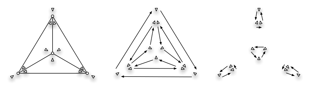
Hypermaps are the primary combinatorial object used by Gonthier in the formalization of the Four-Color theorem in Coq [9]. Hypermaps, by being purely combinatorial, are more convenient to represent on a computer than planar graphs.
Not all hypermaps arise from a planar graph in this way. Those that do have two special properties. They are involutive and planar in the following sense. The definition of planar hypermap is the standard condition on the Euler characteristic, translated into the language of hypermaps.
Definition 7.1.1.
- •
The hypermap is involutive, if is an involution:
- •
The hypermap is planar, if
where denotes the cardinality of .
7.2 Packings and hypermaps
Let be a packing satisfying . The graph is planar. Assume that is biconnected. This subsection describes in greater detail the hypermap attached to .
For each , let
For each , there is a half-plane containing , bounded by the line through . There is a cyclic order on the half-planes , moving in a counterclockwise circle around the ray emanating from through . Write for the cyclic permutation on , given by this ordering.
Define the set of darts by
Define face, edge, and node permutations on by
A formal calculation shows that is an involutive hypermap.
The nodes of are in bijection with under the correspondence:
The edges of are in bijection with the edges of under the correspondence:
The faces of are in bijection with the faces of under the correspondence:
where is the third component of the four-tuple and each face of is represented as usual as cycle . The set of darts is in bijection with the set of oriented edges of under the correspondence:
The graph is connected. This implies that acts transitively on .
The graph is planar. If are the number of vertices, edges, and faces, then ; or equivalently, . Under the bijections just described, this implies that the cardinalities of these sets satisfy
Thus, the hypermap is planar.
Remark 7.2.1.
In [16], the basic combinatorial structure is called a planar map rather than hypermap. In that article, the combinatorial structure is represented in computer code as a finite set of faces
and each face is represented as a cycle of vertices. This is essentially equivalent to a hypermap. This representation is converted to a hypermap by sending to the dart . There are -choices of which vertex to list first in the cycle, and by taking all choices, darts are obtained. Running through all faces in this way, all darts are constructed. In the opposite direction, an earlier argument describes how a face of the hypermap gives a face of , expressed as a cycle.
7.3 Tameness
This subsection defines a collection of hypermaps called tame Voronoi hypermaps. The classification of these hypermaps, up to isomorphism, is one of the main steps of the proof of the Dodecahedral conjecture. Bauer and Nipkow have formally proved the classification in Isabelle [29]. This Isabelle proof was originally designed for the classification of the sphere packing problem. Nipkow and McLaughlin have modified that proof to cover the Dodecahedral conjecture as well. The modified Isabelle proof is found at [26].
Let be a hypermap. A face of (that is, an orbit of under ) is said to be a triangle, quadrilateral, pentagon, etc. if the cardinality of the orbit is , , , respectively. Two nodes are said to be adjacent if there is an edge of such that belongs to one of the nodes and belongs to the other.
Let be a node of (that is, an orbit of under ). A node is said to have type , if the cardinality of is and if there are triangular faces, quadrilateral faces, and other faces that share a dart with . The cardinality of a node is also called its degree.
| 0 | 1 | 2 | 3 | 4 | |
|---|---|---|---|---|---|
| 0 | * | * | * | 0.093 | 0.125 |
| 1 | * | * | 0.092 | 0.093 | * |
| 2 | * | 0.133 | 0.062 | * | * |
| 3 | * | 0.043 | 0.118 | * | * |
| 4 | 0.053 | 0.051 | * | * | * |
| 5 | 0.004 | * | * | * | * |
| 6 | 0.121 | * | * | * | * |
| 7 | * | * | * | * | * |
Define constants by Table 1. If falls outside this table, or if the entry is marked , then set . Let , , be the collection of constants defined in Theorem 6.1.
A weight assignment of a hypermap is a function that is constant on faces: for . A weight assignment is said to be a Voronoi weight assignment if the following properties hold:
- 1.
If the face containing has cardinality , then . (In particular, for all .)
- 2.
Let be any face with cardinality . Let . Let be a set of nodes, each meeting , such that no two are adjacent to one another. Assume that the type of each node of is . Let ; that is, the set of darts in nodes in except those in . Let be the cardinality of . Then
- 3.
If the node of has type and degree , then
The total weight of a weight assignment is defined to be
where is a set of representatives of the orbits of under .
Definition 7.3.1.
is said to be a tame Voronoi hypermap if the following conditions hold.
- 1.
is an involutive, planar hypermap.
- 2.
is connected. That is, is a single orbit under .
- 3.
(Simple face) Every face of meets every node of in at most dart.
- 4.
The number of nodes is at least .
- 5.
The cardinality of each face of is at least and at most .
- 6.
(Triangle types) Let be any three nodes of such that is adjacent to for each . Then there is a dart such that is a face of .
- 7.
There are never two nodes of type that are adjacent to one another.
- 8.
(Quadrilateral types) Let be any four distinct nodes of such that is adjacent to for (setting ). Then darts can be chosen so that the faces containing fall into one of the four patterns depicted in Figure 6.
- 9.
The cardinality (degree) of a node of type is at most five if .
- 10.
The degree of each node of is at least and at most .
- 11.
There exists a Voronoi weight assignment of total weight at most .

7.4 Classification
Two hypermaps and are properly isomorphic if there is a bijection between and that is equivariant for the face, node, and edge permutations. Each hypermap has a mirror image:
An improper isomorphism between two hypermaps is a proper isomorphism between one hypermap and the mirror image of the other. Two hypermaps are isomorphic if there is a proper or improper isomorphism between the two hypermaps. If a hypermap is involutive or planar, then so is every isomorphic hypermap.
There is an archive of tame Voronoi hypermaps [26]. This archive contains hypermaps.
Theorem 7.1.
If is a tame Voronoi hypermap, then it is isomorphic to some hypermap in the archive.
The proof of this theorem relies on the piece of computer code described in Section 3.4. The reader is referred to that section for a description of the details of the theorem.
7.5 Counterexamples are tame Voronoi hypermaps
The following theorem proves that every potential counterexample to the Dodecahedral conjecture gives a tame Voronoi hypermap. In particular, the classification of tame Voronoi hypermaps gives an explicit case enumeration of the possible combinatorial structures of a counterexample. The following section will eliminate each case in the enumeration. This will eliminate all possible counterexamples to the Dodecahedral conjecture.
Theorem 7.2.
Assume that is a counterexample to the Dodecahedral conjecture. Without loss of generality, assume that ; that the cardinality of is at least ; and that is biconnected. Let be the hypermap attached to the graph . For every dart in face , set
Then is a tame Voronoi hypermap and is a Voronoi weight assignment on of total weight at most .
Since the definition of tame Voronoi hypermap is a long enumeration of different properties, the proof of this theorem breaks into a long enumeration of lemmas, each establishing one property. The statement of the theorem specifies the weight assignment . The verification that is a Voronoi weight, breaks into separate lemmas for each property in the definition. The article [16] devotes many pages to the proofs of these lemmas. This articles sketches the proofs and refers the reader to the fuller version for details. Turn to an item by item discussion of the properties. The first several are elementary.
7.5.1 Involutive
The hypermap is involutive and planar. This has been established in Section 7.2.
7.5.2 Connected
The set of darts is a single orbit under . This is also contained in Section 7.2. It follows directly from the connectedness of .
7.5.3 Simple
Every face of meets every node of in at most dart. This is a direct consequence of the biconnectedness of . Indeed, if by following the face permutation , the darts lie at the same node ; then is an articulation vertex of , and the graph is not biconnected.
7.5.4 Node cardinality
The number of nodes is at least . This is a consequence of the assumption that the cardinality of is at least and the bijection in Section 7.2 between nodes of the hypermap and .
7.5.5 Face cardinality
The cardinality of each face of is at least and at most . By definition, the face map on a dart takes the form
| (20) |
In a biconnected graph with more than two vertices, every vertex has degree at least two. Thus every node of the hypermap has degree at least two. Thus, and . Also, , which does not contain . Thus, the form of , and in (20) shows these darts are distinct, and the face contains at least three distinct darts.
If some face of has cardinality at least , then by Theorem 6.1
Thus, is not a counterexample, as was assumed.
7.5.6 Triangle types
Let be any three nodes of such that is adjacent to for each . Then there is a dart such that is a face of . This is a restatement of Lemma 5.3.2 in terms of the combinatorial properties of hypermaps.
7.5.7 Adjacent degrees
There are never two nodes of type that are adjacent to one another. If there are two adjacent nodes of type , then the graph takes the shape of Figure 7. This is an impossible configuration in a packing for purely geometric reasons. It has nothing to do with the value of and volumes of truncated Voronoi cells. The impossibility proof appears as [16, Lemma 3.8]. It is a reparametrization of [13, Prop.4.2]. This is one of the most delicate reparametrizations.

7.5.8 Quadrilateral types
Let be any four distinct nodes of such that is adjacent to for (setting ). Then darts can be chosen so that the faces containing fall into one of the four patterns depicted in Figure 6. Let be the spherical graph on the vertex set with edges for . Then by Jordan curve theorem for polygons, consists of two connected components. The result of [16, Lemma 3.8] cited in the previous proof states more precisely that exactly one connected component of has solid angle less than , and that contains at most one point. If is empty, then the first pattern of Figure 6 occurs.
In remaining cases, contains a single point . Again, by the Jordan curve theorem and the planarity of , all edges in have the form for . Section 7.5.5 shows that each node has degree at least . Thus, is adjacent to , , or of the vertices . Figure 6 gives all such connection patterns of with , except the one shown in Figure 8.

Thus, it is enough to show that pattern of Figure 8 does not occur in any counterexample to the Dodecahedral conjecture. This graph contains a triangle and a pentagon , with corresponding standard components and . An important estimate [16, Lemma 10.1] gives that
If there is some other face with sides, then Theorem 6.1 gives
Otherwise, pick any four vertices in other than . Let be the standard components indexed by triangles of that contain one of these four vertices. Another estimate [16, Lemma 5.2] gives
This shows that is not a counterexample.
7.5.9 Degree
The degree of a node of type is at most five if . Indeed, it is a direct consequence of the inequalities of [26] that if , for , are the standard components of the faces around the node, then
7.5.10 Degrees
7.5.11 Total weight
There exists a Voronoi weight assignment of total weight at most . By definition, a counterexample is a packing such that
| (21) |
The set of standard components is in bijection with the faces of . By the definition of in the statement of the theorem, (21) can be rewritten as
This is exactly what it means for to have total weight at most .
7.5.12 Voronoi weight
The weight assignment is a Voronoi weight. This can be expressed as the following claims.
- 1.
If the face has cardinality then .
- 2.
Let be any face with cardinality . Let . Let be a set of vertices of , such that no two are adjacent to one another. Assume that the type of each node of is . Let be the set of triangles at the vertices . that is, the set of darts in nodes in except those in . Let be the cardinality of . Then
(22) - 3.
If the node of has type and degree , then
(23)
The first of these claims is a direct consequence of Theorem 6.1. Consider the second claim. Form the graph and partition into subcomponents by the algorithm described in Section 6.3. A result in Tarski arithmetic states that two internal pairs and with do not cross each other in the sense of Section 6.3 [16, Sec. 7.2.1]. It follows that every internal pair such that forms an edge of the graph . The bound on is obtained by superadditivity, from a collection of inequalities for each subcomponent.
Let be a node in . Let be the dart in at node . Let be the subcomponent indexed by the triangle in . At a node of type , by angle considerations, the pair is necessarily internal. Let be the standard components indexed by the four triangles at . By summing over , the following two inequalities imply (22).
- 1.
If , then
- 2.
If , then
These inequalities are obtained by summing over interval arithmetic inequalities for each term . A detailed proof appears at [16, Theorem 8.1].
Consider the final claim. The argument at [16, p.14] goes as follows. Let be a vertex. To have type means that there are triangles and quadrilaterals in the graph at the vertex . Interval arithmetic can be used to compute lower and upper bounds on the azimuth angles when is a triangle or quadrilateral. These bounds are [16, F.2.1,F.4]
| (24) |
By the bounds on the azimuth angles, this equality can only be satisfied for special . Anything else is a geometric impossibility. The feasible pairs are listed in [16, Lemma 6.1]. According to this list, and .
Interval arithmetic methods establish a list of nonlinear inequalities relating to when is a triangle or quadrilateral [26]. If free variables and are substituted into these inequalities for and , then the resulting inequalities are linear in these variables. A system of linear inequalities results. (This is the method of linear relaxation.) A lower bound on the left-hand side of (23) is the solution of the linear program
subject to
and to the system of linear inequalities. The linear program is run for each and a constant slightly smaller than the minimization was picked. This gives the table of values.
If is a counterexample to the Dodecahedral conjecture with a vertex of type , then
An inspection of the list of constants in the table shows that that this implies that . That is, the degree of every vertex of type is at most . This is the property needed in Section 7.5.10.
8 Linear Programs
This section discusses Theorem 8.1. It is one of the main steps in the proof of the Dodecahedral conjecture. The discussion begins with the terminology used in the statement of the theorem.
Definition 8.0.1.
A hypermap system is a pair , where is a hypermap, and is a finite set constraints on . More precisely, let be the vector space of real-valued functions on . Each is a boolean valued function for some . (Assume is independent of ).
The hypermap system is said to be feasible, if there is some such that holds for all . Otherwise, the system is infeasible.
In our hypermap systems, the constraints are generated from a list of about one hundred generic parametrized constraints, with a parameter running over the darts in a hypermap. For example, a parameterized constraint might be interpreted as an inequality relating , the solid angle of , and azimuth angles, whenever is a triangular face containing the dart . As runs over the darts in a hypermap , the generic constraint evaluates to a constraint for each dart in every triangular face of , yielding dozens of particular constraints for . We do not list the generic constraints here, but they appear in [16] and also at [26].
For each tame Voronoi hypermap , the generic constraints specialize to a particular set of constraints . Each set contains about constraints. The hypermap systems arising in this way are called Voronoi hypermap systems.
Theorem 8.1.
Let be any tame Voronoi hypermap. Then is infeasible.
This proof is carried out by computer as a collection of linear programs. This is one of the three major parts of the proof of the Dodecahedral conjecture that have been carried out by computer. This article describes the relationship between the feasibility of and a linear programming feasibility problem. It also describes some details of the implementation of the code.
Section 7.4 enumerates of all tame Voronoi hypermaps. Thus, the proof of Theorem 8.1 may proceed case by case. Let’s focus attention for a moment on one tame Voronoi hypermap and the corresponding Voronoi hypermap system . A simple strategy will show that it is infeasible. For some , each constraint is a function on , where is the vector space of real-valued functions on . Thus, can be identified with , where . An inspection of the form of the generic constraints described above reveals they all have a very special form. They are all linear constraints on .
Some of the linear constraints carry guard conditions. That is, some constraints have the form
| (25) |
for , and various matrices and vectors . (The vector inequality means that for every component of the vectors .) The constraint is called a guard condition. Variations are allowed in which some of the inequalities in the guard condition are weak and some of the inequalities in the consequent are strict.
The collection of all inequalities that do not have a guard condition is a system of linear inequalities. Standard linear programming packages can be used to determine whether this system of linear inequalities has a feasible solution. If this linear program is infeasible, then the hypermap system is clearly also infeasible. When this happens, a proof of the infeasibility of results.
When this fails, the constraints with guard conditions are used. The introduction of a constraint that has a nontrivial guard condition involves multiple steps. The constraint (25) can be rewritten in logically equivalent form as
where and are the rows of and . Taking each disjunct in turn, one linear inequality at a time is added to the system of linear inequalities, and the resulting system is shown to be infeasible. When each systems are infeasible, then itself is infeasible.
This discussion may give the impression that a great many linear programming feasibility problems are created in this manner. In practice, nearly all of the hypermap systems are eliminated in the first pass, without requiring recourse to the guard conditions.
8.1 Counterexample implies feasibility
Theorem 8.2.
Let be a counterexample to the Dodecahedral conjecture. Let be the Voronoi hypermap system attached to . Then is feasible.
Proof.
It is enough to give some assignment of such that holds for all . Each is a real-valued function on darts. The notation for the functions has been set up in a way that suggests the assignment. Let be a dart. Let be the face containing . Make the following settings. The first row of this table gives the functions in the notation of [26]. The second row gives the real number .
All of the predicates can be shown to hold for this assignment, either as a consequence of definitions, as consequences of geometrical facts, or as consequences of interval arithmetic calculations.
The interval arithmetic calculations for the predicates with guard conditions were verified in two stages. The polygonal face is triangulated, and the standard component is partitioned in a corresponding way into parts . In the first stage, the guard hypotheses were used to obtain interval arithmetic bounds on the lengths of the internal edges of the triangulation. In the second stage, these edge length bounds are used as hypotheses in further interval arithmetic bounds that give lower bounds on . Then
This becomes a general predicate on darts of the form:
∎
Since no tame Voronoi hypermap is feasible, by the argument of Section 2.2 the Dodecahedral conjecture is established.
Thanks
This research was supported by NSF grant 0503447. Many of the nonlinear inequalities for the proof of the Dodecahedral conjecture were proved by computer by S. Ferguson. We wish to thank him for his generous support of this project. We wish to thank C. Anghel for helpful comments.
References
- [1] G. Alefeld and J. Herzeberger. Introduction to Interval Computations. Academic Press, 1983.
- [2] G. Bauer. Formalizing Plane Graph Theory – Towards a Formalized Proof of the Kepler Conjecture. PhD thesis, Technische Universität München, 2006.
- [3] Y. Bertot and P. Castéran. Interactive theorem proving and program development: Coq’Art: the Calculus of Inductive Constructions. Texts in theoretical computer science. Springer-Verlag, 2004.
- [4] K. Bezdek. Isoperimetric inequalities and the dodecahedral conjecture. In International Journal of Mathematics, volume 8/6, pages 759–780, 1997.
- [5] K. Bezdek. Sphere packings in -space. In Proceedings of COE Workshop on Sphere Packings, pages 32–49. Kyush University Press, 2004.
- [6] R. H. Byrd, J. N. Ocedal, and R. A. Waltz. Knitro: An integrated package for nonlinear optimization. In G. di Pillo and M. Roma, editors, Large-Scale Nonlinear Optimization, pages 35–59. Springer-Verlag, 2006.
- [7] G. E. Collins. Quantifier elimination for real closed fields by cylindrical algebraic decomposition. In H. Brakhage, editor, Automata Theory and Formal Languages, volume 33 of Lecture Notes in Computer Science, pages 134–183, Berlin, 1975. Springer-Verlag.
- [8] B. Collins-Sussman, B. W. Fitzpatrick, and C. M. Pilato. Version Control with Subversion. O’Reilly & Associates, Inc., 2004.
- [9] G. Gonthier. A computer-checked proof of the four colour theorem. Unpublished manuscript, 2005.
- [10] Google Project Hosting. http://code.google.com/hosting.
- [11] T. Hales. The Flyspeck Fact Sheet, 2003 (revised 2007). http://code.google.com/p/flyspeck/wiki/FlyspeckFactSheet.
- [12] T. Hales. The status of the Kepler conjecture. In Mathematical Intelligencer, volume 16/3, pages 47–58, 1994.
- [13] T. Hales. Sphere packings I. In Discrete and Computational Geometry, volume 17, pages 1–51, 1997.
- [14] T. Hales. Some algorithms arising in the proof of the Kepler conjecture. In Discrete and Computational Geometry, volume 25, pages 489–507, 2003.
- [15] T. Hales. The Flyspeck Project, 2007. http://code.google.com/p/flyspeck.
- [16] T. Hales and S. McLaughlin. A proof of the Dodecahedral conjecture (1998 version). http://arxiv.org/abs/math/9811079v2.
- [17] T. Hales and S. McLaughlin. A proof of the Dodecahedral conjecture (2002 version). http://arxiv.org/abs/math/9811079v1.
- [18] T. C. Hales and S. P. Ferguson. The Kepler conjecture. Discrete and Computational Geometry, 36(1):1–269, 2006.
- [19] E. Harshbarger. Saturated packings and Voronoi cells, 1996. http://www.ericharshbarger.org/voronoi.html.
- [20] J. F. Hart et al. Computer Approximations. John Wiley & Sons, 1968.
- [21] L. Hörmander. The Analysis of Linear Partial Differential Operators II, volume 257 of Grundlehren der mathematischen Wissenschaften. Springer-Verlag, 1983.
- [22] W.-Y. Hsiang. On the sphere packing problem and the proof of Kepler’s conjecture. In International Journal of Mathematics, volume 4/5, pages 739–831, 1993.
- [23] IEEE Standards Committee 754. IEEE Standard for binary floating-point arithmetic, ANSI/IEEE Standard 754-1985. Institute of Electrical and Electronics Engineers, New York, 1985.
- [24] R. B. Kearfott. Rigorous Global Search: Continuous Problems. Kluwer, Dodrecht, Netherlands, 1996.
- [25] C. Lawrence, J. L. Zhou, and A. L. Tits. A C code for solving (large scale) constrained nonlinear (minimax) optimization problems, generating iterates satisfying all inequality constraints. Technical Report TR-94-16r1, Institute for Systems Research, University of Maryland, 1997. http://www.aemdesign.com/download-cfsqp/cfsqp-manual.pdf.
- [26] S. McLaughlin. KeplerCode: computer resources for the Kepler and Dodecahedral Conjecutures. http://code.google.com/p/kepler-code/.
- [27] D. J. Muder. Putting the best face on a voronoi polyhedron. In Proceedings of the London Mathematical Society, volume 3/56, pages 329–348, 1988.
- [28] D. J. Muder. A new bound on the local density of sphere packings. In Discrete and Computational Geometry, volume 10, pages 351–375, 1993.
- [29] T. Nipkow, G. Bauer, and P. Schultz. Flyspeck I: Tame Graphs. In U. Furbach and N. Shankar, editors, International Joint Conference on Automated Reasoning, volume 4130 of Lecture Notes in Computer Science, pages 21–35. Springer-Verlag, 2006.
- [30] S. Obua. Flyspeck II: The Basic Linear Programs. PhD thesis, Technische Universität München, 2008.
- [31] L. Paulson. Isabelle: A Generic Theorem Prover, volume 828 of Lecture Notes in Computer Science. Springer-Verlag, 1994.
- [32] W. H. Press et al. Numerical Recipes in C, volume Chapter 20. Less-Numerical Algorithms. Cambridge University Press, second edition, 1992.
- [33] C. A. Rogers. The packing of equal spheres. In Journal of the London Mathematical Society, volume 3/8, pages 609–620, 1958.
- [34] L. F. Tóth. Uber die dichteste kugellagerung. In Mathematische Zeitschrift, volume 48, pages 676–684, 1943.
- [35] L. F. Tóth. Regular Figures. Pergamon Press, Oxford-London-New York, 1964.
- [36] L. F. Tóth. Lagerungen in der Ebene auf der Kugel und im Raum. Springer-Verlag, Berlin-New York, second edition, 1972.
- [37] R. Zumkeller. Formal global optimisation with taylor models. In U. Furbach and N. Shankar, editors, International Joint Conference on Automated Reasoning, volume 4130 of Lecture Notes in Computer Science, pages 408–422. Springer-Verlag, 2006.
- [38] R. Zumkeller. Rigorous Global Optimization. PhD thesis, Ècole Polytechnique, 2008.