On the Distribution of the Length of the Longest Increasing Subsequence
of Random PermutationsThanks: The authors would like to acknowledge
many extremely useful and enlightening conversations with Persi Diaconis and
Andrew Odlyzko. Special thanks are due
to Andrew Odlyzko and Eric Rains for providing us with
the results of their Monte Carlo simulations. Thanks: The work of the second author was supported in part by NSF
grant #DMS-9500867.Thanks: The work of the third
author was supported in part by the Swedish Natural Research Council
(NFR)
Jinho Baik
Address: Courant Institute of Mathematical Sciences, New York
Current address: Email address: baik@cims.nyu.edu, Percy Deift
Address: Courant Institute of Mathematical Sciences, New York
Email address: deift@cims.nyu.edu and Kurt Johansson
Address: Royal Institute of Technology, Sweden
Email address: kurtj@math.kth.se
Date: July 2, 1998 ; March 25, 1999 (revised)
Abstract.
The authors consider the length, , of the length of the longest
increasing subsequence of a random permutation of numbers.
The main result in this paper is a proof that the distribution function
for , suitably centered and scaled, converges to the
Tracy-Widom distribution [TW1] of the largest eigenvalue of a random
GUE matrix.
The authors also prove convergence of moments.
The proof is based on the steepest decent method for Riemann-Hilbert
problems, introduced by Deift and Zhou in 1993 [DZ1] in the context
of integrable systems.
The applicability of the Riemann-Hilbert technique depends, in turn,
on the determinantal formula of Gessel [Ge] for the Poissonization
of the distribution function of .
Key words and phrases:
Random permutations, orthogonal polynomials, Riemann-Hilbert
problems, random matrices, steepest descent method
1991 Mathematics Subject Classification
05A05, 15A52, 33D45, 45E05, 60F99
1. Introduction
Let be the group of permutations of .
If , we say that
is an increasing subsequence in if and
.
Let be the length of the longest increasing subsequence.
For example, if and is the permutation
(in one-line notation
: thus , , ), then the longest
increasing subsequences are and , and .
Equip with uniform distribution,
where .
The goal of this paper is to determine the asymptotics of
as .
This problem was raised by Ulam in the early 60’s [Ul],
and on the basis of Monte Carlo simulations, he
conjectured that the limit
(1.1)
exists.
(Here denotes the expectation value with respect
to the distribution function .)
The problem of proving the existence of this limit and the computation
of has became known as “Ulam’s problem”.
An argument of Erdös and Szekeres [ES] shows that
, so that if the limit
exists, then .
Subsequent numerical work by Baer and Brock [BB]
in late 60’s suggested that value of is 2.
The existence of the limit was rigorously
established by Hammersley [Ha] in 1972.
In [LS], Logan and Shepp proved that and simultaneously
Vershik and Kerov [VK1] (see also [VK2]) showed that ,
thus settling Ulam’s problem.
Alternative proofs of Ulam’s problem are due to Aldous and Diaconis
[AD], Seppäläinen [Se1] and Johansson [Jo1].
Over the years, various conjectures have been made concerning
the variance of , and Monte Carlo simulations of
Odlyzko and Rains beginning in 1993, indicated that
(1.2)
for some numerical constant .
Also Odlyzko and Rains computed to higher order
and found
(1.3)
where .
Further historical information on Ulam’s problem, together with some
discussions of the methods used by various authors, can be found
in [AD] and [OR]
Before stating our results, we need to define the Tracy-Widom
distribution [TW1] (see below).
Let be the solution of the Painlevé II (PII) equation,
(1.4)
where is the Airy function.
The (global) existence and uniqueness of this solution was first
established in [HM] :
the asymptotics as are,
(1.5)
(see, for example, [HM], [IN], [DZ2]).
Recall [AS] that as .
Define the Tracy-Widom distribution
(1.6)
From (1.5) and (1.6), ,
as and
as , so that is indeed a distribution function.
Our first result concerns the convergence of in distribution
after appropriate centering and scaling.
Theorem 1.1.
Let be the group of all permutations of numbers
with uniform distribution and let be the length of
the longest increasing subsequence of .
Let be a random variable whose distribution function is .
Then, as ,
i.e.
In order to show that the moments of converge to the
corresponding moments of we need estimates for the distribution
function of for large . From the large
deviation formulas for (see below), we expect that
(resp., )
should go to zero rapidly as (resp., ).
In fact, we will prove that, for
sufficiently large, there are positive constants and
such that
(1.7)
if , and
(1.8)
if .
Together with Theorem 1.1 these estimates yield
Theorem 1.2.
For any , we have
where denotes expectation with respect to the distribution
function . In particular,
(1.9)
and
(1.10)
If one solves the Painlevé II equation (1.4) numerically
(see, [TW1]), and then
computes the integrals on the RHS of the formulae of (1.9)
and (1.10), one obtains the values 0.8132 and -1.7711
which agree with
and in (1.2) and (1.3) respectively,
up to two decimal places.
The distribution function in Theorems 1.1 and 1.2
first arose in the work of Tracy and Widom on
the Gaussian Unitary Ensemble (GUE) of random matrix theory.
In this theory (see, e.g., [Me]), one considers
hermitian matrix with probability density
where is the normalization constant.
In [TW1], Tracy and Widom showed that
as the size of the hermitian matrices increases,
the distribution of the (properly centered and scaled) largest
eigenvalue of a random GUE matrix
converges precisely to !
In other words, properly centered and scaled, the length of the longest
increasing subsequence for a permutation , behaves statistically
for large like the largest eigenvalue of a random GUE matrix
(see the Appendix for an intuitive argument).
In [TW1], the authors also computed the distribution functions of
the second, third, largest eigenvalues of such random matrices,
and the question arises whether such distribution functions describe
the statistics of quantities identifiable in the random permutation
context.
Recall the Robinson-Schensted correspondence
(see, e.g., [Sa], and also Section 5.1.4 in [Kn])
which establishes a bijection from
to pairs of Young tableaux with shape shape.
Under this correspondence, the number of boxes in the first row
of (equivalently ) is precisely ,
(see, [Sa], [Kn]).
In other words, the results on can be rephrased as results on
the statistics of the number of boxes in the first row of Young tableaux.
Monte Carlo simulations of Odlyzko and Rains [OR] indicate that ,
the number of boxes in the second row of
(equivalently ) behaves
statistically for large , like the second largest eigenvalue of a
random GUE matrix.
More precisely, their simulations indicate that
and
These values agree, once again, to two decimal places with
the mean and variance of the suitably centered
and scaled second largest eigenvalue of a GUE matrix,
as computed in [TW1].
Presumably, the number of boxes in the third row of should
behave statistically like the third largest eigenvalue of a GUE matrix
as , etc.
In recent work [BDJ], the authors have shown that this
conjecture is indeed true for the second row.
Also, beautiful results of Okounkov [Ok],
using arguments from combinatorial topology, have now provided an elegant
basis for understanding the relationship between the statistics
of Young tableaux and the eigenvalues of random matrices.
Over the last year, many other intriguing results have been obtained
on a variety of problems arising in mathematics and mathematical
physics, which are closely related to, or motivated by,
the longest increasing subsequence problem.
We refer the reader to
[TW2], [Bo], [Jo2, Jo3] and [BR].
The function is a distribution function (in ) of
a random variable coming from a superadditive process
introduced by Hammersley in [Ha], and used by him to show that the
limit (1.1) exists. The random variable is defined as
follows.
Consider a homogeneous rate one Poisson process in
the plane and let denote the maximum number of points in
an up-right (increasing) path through the points starting at
and ending at . For more details see
[AD] and [Se2], and for a generalization to the non-homogeneous case
see [DeZe1]. Theorem 1.1 and 1.2
hold for the random variable
as .
Referring to the “de-Poissonization”
Lemmas 8.2 and 8.3
below, we see that it is easy to recover the asymptotics of
as from the knowledge of for
.
In other words, in order to compute the asymptotics of ,
we must investigate
the double scaling limit of when
and , and this is
the technical thrust of the paper.
To this end we use the following representation for ,
(1.12)
where denotes the Toeplitz determinant
with weight function
on the unit circle, (see, e.g.,[Sz1]).
The above formula follows from work of Gessel in [Ge] using well known
results about Toeplitz determinants.
As noted in [Jo1], the formula can also be proved using
the following representation for , ,
discovered by [OPWW],
(1.13)
In addition, an earlier result of Diaconis and Shahshahani ([DS]) shows
that the above formula (1.13) is true also in the case
when .
Inserting (1.13) into (1.11), we obtain
(1.14)
which is precisely (1.12) by standard methods in the theory of
Toeplitz determinants (see, [Sz1]).
An additional proof of (1.12) can be found in [GWW], and
also an alternative derivation of formula (1.13) is given
in [Ra].
For the convenience of the reader we provide (yet another)
proof of (1.12)
in the Appendix to this paper.
Using the integral representation (1.12),
Johansson ([Jo1]) proved
the following bound for :
for any given , there exist and such that
(1.15)
This information and the de-Poissonization Lemma 8.2
are enough to give a new proof ([Jo1]) that
(1.16)
The first estimate in (1.15) is a consequence of the following lower
tail large deviation formula for ,
(1.17)
if .
For the upper tail Seppäläinen in [Se2] used
the interacting particle system implicitly
introduced by Hammersley in [Ha] to show that
(1.18)
if . We note that Hammersley’s interacting particle system was also used
earlier by Aldous and Diaconis in [AD].
The super-additivity of the process described above implies that we
actually have, see [Se2] and also [Ki],
(1.19)
if is a positive integer and . This estimate can be used
to show (1.8), but in this paper we will give an independent proof
of (1.8).
The large deviation formula (1.18) implies, via a de-Poissonization
argument, that for ,
(1.20)
For the lower tail the large deviation formula for is not the
same as for , the Poissonized case. Deuschel and Zeitouni
in [DeZe2] use combinatorial and variational
ideas from Logan and Shepp [LS] to prove that
(1.21)
if , where
(1.22)
For the lower tail we have no analogue of (1.19). The rate functions
and are related via a Legendre transform, see [Se2].
The above results show clearly that the distribution function for
is sharply concentrated in the region
for
any , and they can be used to see heuristically that the
variance for should be of order , see [Ki].
As is well known (see, [Sz1]) the Toeplitz determinant
in (1.12)
is intimately connected with the polynomials
,
which are orthonormal with respect to
the weight
on the unit circle,
(1.23)
The leading coefficient can be expressed
in terms of Toeplitz determinants,
(1.24)
where .
But by Szegö’s strong limit theorem ([Sz2])
for Toeplitz determinants,
, and hence
(1.25)
Therefore, if one can control the large
behavior of
for all , one will control the large
behavior of .
The key point in our analysis is that
can be expressed in terms of
the following Riemann-Hilbert Problem (RHP) :
Let be the unit circle oriented counterclockwise.
Let be the matrix-valued function satisfying
(1.26)
where and denote the limit from inside and outside of
the circle respectively, and ,
so that .
Here is the identity matrix.
This RHP has a unique solution
(see (4.1) below), and the fact of the matter is that
(1.27)
where is the -entry of the solution
at .
In [DZ1] and [DZ2], Deift and Zhou introduced a steepest descent
type method to compute the asymptotic behavior of RHP’s containing
large oscillatory and/or exponentially growing/decaying factors as in (1.26).
This method was further extended in [DVZ1] and eventually placed
in a very general form by Deift, Zhou and Venakides in [DVZ2],
making possible the analysis of the limiting behavior
of a large variety of asymptotic problems in pure and applied mathematics
(see, e.g., [DIZ]).
As we will see, the application of this method to (1.26) makes it possible
to control the large behavior of .
The calculation in this paper have many similarities to the computations
in [DKMVZ], where the authors use the steepest descent method to obtain
Plancherel-Rotach type asymptotics for polynomials orthogonal with respect of
varying weights, on the real line, and hence to prove
universality for a class of random matrix models.
The Riemann-Hilbert formulation of the theory of orthogonal
polynomials on the line is due to Fokas, Its and Kitaev ([FIK]) :
the RHP (1.26) is an adaptation of the construction in [FIK]
to the case of orthogonal polynomial with respect to a weight
on the unit circle.
This paper is arranged as follows.
In Section 2, we discuss of some of the basic theory of RHP’s
and also provide some information on the RHP associated with the PII equation.
This information will be used in the construction of an approximate solution,
i.e. a parametrix,
for the RHP (1.26) in
subsequent sections. The appearance of the
PII equation in the limiting distribution
for
originates in this construction of the parametrix.
A connection of to Toda lattice and the Painlevé III equation
is presented in Section 3.
Section 4 is the starting point for the
analysis of the RHP (1.26).
In this section, (1.26) is transformed into an equivalent
RHP via
a so-called -function.
The role of -function, first introduced in [DZ2], and then
analyzed in full generality in [DVZ2],
is to replace exponentially growing terms in a RHP by oscillatory or
exponentially decreasing terms.
It turns out that in the case of (1.26), as in [DKMVZ1], the
-function can be constructed in terms of an associated equilibrium
measure as follows,
(1.28)
The measure is the unique minimizer of the following variational problem :
(1.29)
where
(1.30)
and .
The variational problem (1.29) describes the equilibrium configuration
of electrons, say, confined to the unit circle with Coulomb interactions,
and acted on by an external field .
It turns out that the support of the equilibrium measure depends
critically on the quantity
(1.31)
We need to distinguish these two cases, and .
As noted by Gross and Witten ([GW]), and also by Johansson
([Jo1]), the point corresponds
to a (third order) phase transition for a statistical system
with partition function (1.14).
The first case, when ,
is discussed in
Section 5, and the second case,
when , is discussed
in Section 6.
The principal results of the above two sections are summarized in
Lemmas 5.1 and 6.3.
We obtain full asymptotics of
for when .
In Section 7, by summing up
for all , we obtain the asymptotics of
in Lemma 7.1.
The relation between and
(de-Poissonization) is discussed in
Section 8.
Finally, the proofs of Theorem 1.1 and 1.2 are given in
Section 9.
Notational remarks : The primary variables in this paper are ,
and .
The letters , denote general positive constants.
Rather than introducing many such constants
we always interpret in a general way.
For example, we write , etc.
We will also use certain auxiliary positive parameters
.
If a constant depends on some of these parameters, we indicate
this explicitly, for example, .
In addition to the standard big notation, we also use a notation
.
Thus means , where
is independent of .
On the other hand, means
,
where depends on at least one of the parameters
.
In the estimates that follow we will often claim that an inequality
is true “as ”.
For example, in (7.3) below, we say that
as .
This mean that there exists a number , say, which may
depend on all the other relevant constants in the problem,
such that the inequality is true for , etc.
(For this particular inequality the only other parameter is
, but it turns out that the constants , can be
chosen independent of (see below).)
2. Riemann-Hilbert Theory
In this section, we first summarize some basic facts about RHP’s in general,
and then discuss the RHP for the PII equation in some detail.
Basic references for RHP’s are [CG], [GK], and
the material on PII is taken from [DZ2].
Let be an oriented curve in the plane (see,
for example, Figure 1).
Figure 1.
By convention, the -side (resp., -side) of an arc in
lies to the left (resp., right) as one traverses the arc in the direction
of the orientation.
Thus, corresponding to Figure 1, we have Figure 2.
Figure 2.
Let and
be a smooth map from , for some .
If is unbounded, we require that as
along .
The RHP consists of the following (see, e.g., [CG]) :
establish the existence and uniqueness of an matrix valued
function (the solution of the RHP )
such that
(2.1)
Here where
.
The precise sense in which these boundary values are attained, and also
the precise sense in which as , are
technical matters
that should be specified for any given RHP .
In this paper, by a solution of a RHP , we always mean
that
(2.2)
Given , the existence of under appropriate
technical assumptions on and , is in general
a subtle and difficult question.
However, for the RHP (1.26), and hence for all RHP’s obtained by
deforming (1.26) (see, e.g., (4.9)), we will prove the
existence of directly by construction (see, Lemma 4.1) :
uniqueness, as we will see, is a simple matter.
The solution of a RHP can be expressed in terms of
the solution of an associated singular integral equation on
(see, (2.7), (2.8) below) as follows.
Let be the Cauchy operators
(2.3)
where denotes the non-tangential limit from the side
of respectively.
A useful reference for Cauchy operators on curves which may have points of
self-intersection is [GK].
Under mild assumptions on , which will always be satisfied
for the curves that arise in this paper, the non-tangential limits
in (2.3) will exist pointwise a.e. on .
Furthermore, if , , then
the boundary values (appropriately interpreted at the points
of self-intersection)
of
are also taken in the sense of and
.
A simple calculation shows that
(2.4)
Let
(2.5)
be any factorization of .
We assume , and hence , are smooth on , and
if is unbounded, we assume as
along .
Define the operator
(2.6)
By the above discussion, if , then
is bounded from .
Suppose that the equation
(2.7)
has a solution ,
Or more precisely, suppose solves
(2.8)
which is a well-defined
equation in provided that
.
Then the solution of the RHP (2.1) is given by
(see, [CG],[BC])
and similarly , so that a.e. on .
Under the appropriate regularity assumptions on and ,
one then shows that solves the RHP
in the sense of (2.2).
As indicated, the above approach to the RHP goes through for any
factorization .
Different factorization may be used at different points in the
analysis of any given problem (see e.g. [DZ1]).
However, in this paper we will always take , so that
.
Thus always denotes the operator .
In this paper we will not develop the general theory for the solution
of RHP’s, giving conditions under which (2.7) has a (unique)
solution, etc.
Rather, for the convenience of the reader who may not be familiar with
Riemann-Hilbert theory, we will use the above calculations
and computations as a guide,
and verify all the steps directly as they arise.
We now consider the RHP for the PII equation
([FN], [JMU] : see also [IN], [FZ], [DZ2]).
We will consider two equivalent versions of the RHP for PII.
These two RHP’s
will be used in the later sections for the construction of parametrices
for the solution of (1.26).
Let denote the oriented contour consisting of 6 rays
in Figure 3.
Thus ,
with associated jump matrix ,
where the monodromy data and are
complex numbers satisfying the relation
(2.10)
Figure 3. and
For and , set
(2.11)
where
(2.12)
The contour consists precisely of the set .
This implies, in particular, that .
For example, as along the real axis,
is oscillatory
(on the other rays, , ,
could grow), and so we cannot expect that the RHP
has a solution in the sense of (2.2).
However, if we rotate in the clockwise direction by any
angle , , , then it is
easy to see that ,
and we may expect that the RHP
has a solution in the sense of (2.2).
Moreover, as is analytic, it is clear that if one can
solve for some ,
then one can solve
for any other , and the solution of the
-problem can be obtained from the -problem
by an analytic continuation, and vice versa.
So suppose that for some fixed , and for
,
is a ( matrix) solution of the RHP
,
(2.13)
in the sense of (2.2).
Let denote the residue at of
, given by
where (resp., ) denotes
the -entry (resp, -entry) of .
It is easy to see that , and hence in (2.14),
is independent of the choice of
A solution of the RHP
for some , hence for all , may not exist
for all satisfying (2.10) and .
A sufficient condition (see [FZ])
for the RHP to have a unique solution (in the sense of (2.2))
for all , is that
In this paper, we need the singular case
(2.15)
Figure 4. case ; and
The latter condition implies that
there is no jump across the rays ,
and we may replace by
as in Figure 4 (note that the orientations across the rays
have been reversed).
As noted in [DZ2], a unique solution in the sense of (2.2)
still exists in this singular case
for all : a proof of this fact is not given in [DZ2],
but can be found in [DKMVZ3 ; nonregular case, Case II].
In addition, the solution has the property that
(2.16)
for any fixed .
As solves (2.13)
in the sense of (2.2), we see
in particular that (2.16) holds up to the boundary in each sector.
The asymptotics of
given in (1.5), is computed in [DZ2] via the above RHP and
from the proof in [DZ2], one learns that
(2.17)
where denotes the -entry of .
Also, using the methods in [DZ2], for example,
one obtains the relation
(2.18)
and verifies directly that is real-valued.
Figure 5. and
For the first of the two equivalent RHP’s advertised above,
we consider Figure 5, which consists of
the real axis (the dotted line), for some
fixed, small (the dashed lines), and a contour
consisting of a pair of curved solid lines.
The contour is of the general shape indicated
in the Figure, with one component in and one component in ,
and we require that is asymptotic to straight lines
lying strictly within
the region .
Together with the line ,
these contours divide
the complex plane into 4 open regions,
, , as shown in Figure 5.
Let be the jump matrix on which is given by
in
and by in .
We define
where the regions , are defined
in Figure 4.
A straightforward calculation with the jump relations for
,
shows that
solves the new RHP
(2.19)
where
and is given in Figure 5.
This deformed RHP is clearly equivalent to the original RHP
for
in the sense that a solution of the one RHP yields a solution
of the other RHP, and vice versa.
Also we have
(2.20)
for the residues of (resp, ) at .
From (2.16),
we see that for any fixed ,
(2.21)
A particular choice of contour will be made in
Section 5 (see below).
Figure 6.
The second of the equivalent RHP’s is restricted to the case ,
and we consider
Figure 6, which consists of the real axis (the dotted line),
for some fixed small
(the dashed lines) and a contour consisting of 5 straight lines, one
finite and four infinite.
The regions , , are the components
of .
The infinite lines make an angle strictly between and
with the real axis.
Set
(2.22)
which is defined to be analytic in , and behaves like
as .
Therefore for any ,
(2.23)
and
(2.24)
We define by
Then from the jump relations for ,
we see that solves the new RHP
in the sense of (2.2),
(2.25)
where is given by
(2.26)
Also we have
(2.27)
for the respective residues of and
at .
Finally, from (2.16) and (2.23),
we see that, for any fixed
(2.28)
3. Connection to the Toda Lattice and the Painlevé III Equation
In this Section, we discuss the connection of the RHP (1.26)
for and the RHP for the Toda lattice
and the Painlevé III equation.
In the RH context, the connection results from
the specific form of the weight, .
Connections can also be seen from the Toeplitz determinant/orthogonal
polynomial point of view as in [PS], [Hi] and [Wi].
The purpose of this short Section is purely to establish the
various connection, but we do not use the results in the sequel.
A simple calculation shows that solves the following RHP,
(3.2)
Once again, the RHP for is equivalent to the RHP for
in the sense that a solution of one problem yields a solution
of the other problem.
Recall that the RHP related to the Toda Lattice problem, for
,
(3.3)
under initial data decaying at infinity is the following (see,e.g.,[Ka]).
Suppose that there are no solitons and denote the
reflection coefficient by , .
Then we find such that
(3.4)
When is even, if we set and in (3.2),
then the RHP is identical with the above RHP
with .
For the connection to the Painlevé III equation,
define
where is analytic in
and real-valued for real .
If we set , then
this is the same RHP for the particular
Painlevé III equation (see [FMZ] for results and notations)
with monodromy data
In the RHP (1.26), we are interested directly in the quantity
, or by (3.1), .
On the other hand, for the Toda lattice and the PIII equation, one is
interested in quantities other than which are
related to the respective RHP’s.
For example, the solution of PIII equation is given by
where , which is clearly different from .
However, the importance of the connection of (1.26) to the RHP’s
for Toda lattice and the PIII equation lies precisely in the fact that
(resp., ) solve differential-difference
(resp., differential) equations which in turn imply that the coefficients
of the generating function , ,
must satisfy a certain class of identities.
We plan to investigate these relations in a later publication.
Finally, note that for PIII, the interesting asymptotic question is
to evaluate the limit , with fixed.
In this paper, as in the Toda lattice, we are interested in the double
limit when and is allowed to vary
(note that in [Ka], the singular case is not
considered).
When , ,
we are in a region where the solution of PIII equation degenerates
to a solution of PII equation, and this explains the appearance of
PII in the parametrix for the solution of of the RHP (1.26).
4. Equilibrium Measure and -function
In this Section, the equilibrium measure is explicitly calculated
for each (Lemma 4.3) and, using this equilibrium measure,
the -function (4.8) is introduced in order to
convert the RHP (1.26)
into a RHP which is normalized to be at .
Let denote the unit circle oriented counterclockwise
and be a non-negative, periodic, smooth
function on .
Let be the -th normalized orthogonal
polynomial with respect to the weight
on the unit circle.
Define the polynomial (see [Sz1]).
We consider the following RHP :
Let be the matrix-valued function satisfying
(4.1)
The following Lemma is the starting point of our calculations.
Lemma 4.1.
(cf. [FIK], [DKMVZ1]) The RHP (4.1) has a unique solution
Proof.
Existence : Using the property of Cauchy operator , where
,
it is a straightforward calculation
to show that the above expression for satisfies the jump condition.
The asymptotics at codes in precisely the fact that the
are the normalized orthogonal polynomials for the weight
.
Uniqueness : Suppose that there is another solution of RHP. Noting
, we have that is entire,
and
as . Therefore by Liouville’s theorem, .
In particular, is invertible.
Now set . Then it has no jump on
hence is entire.
Also, as , and therefore .
∎
From this Lemma, we have
(4.2)
Therefore the RHP (1.26) has a unique solution
and (1.27) is verified.
Again set and
(4.3)
We are interested in the case when and
are of the same order
, or more precisely, .
In this Section, and also in Sections 5 and 6, we consider
the RHP (1.26) with parameter and ,
(4.4)
rather than and .
With fixed, the RHP (4.4) is of the Plancherel-Rotach type
with varying exponential weight
on the unit circle
(see [Sz1], [DKMVZ1]).
Similar problem on the real line is analyzed in [DKMVZ1]
without double scaling limit ( is kept fixed).
Our goal is to find the large behavior of for all .
Figure 7. branch cut of
Let be a probability measure on the unit circle.
Define
(4.5)
where for each , the branch is chosen such that
is analytic in
(see Figure 7)
and for real .
The following Lemma is based on related calculations in [DKM].
Lemma 4.2.
Suppose is an absolutely continuous probability
measure on the unit circle and .
Then has the following properties :
(1)
is analytic in
(2)
On
(3)
as
(4)
is analytic in
(5)
as
(6)
(7)
on where
(8)
on z
Proof.
(i)-(v) are trivial.
For (vi),
using the evenness of .
For (vii), fix .
Then is analytic if and
Note that for ,
This yields
Set
If we show , then (vii) is proved.
Note that (a) ,
(b) and
(c) .
This gives us . But . Therefore
For (viii),
∎
Let be the set of probability measures on .
The equilibrium measure for potential
on the unit circle is defined by the following minimization problem,
(4.6)
The infimum is achieved uniquely (see, e.g. [ST]) at the
equilibrium measure.
Let denote the support of .
The equilibrium measure and its support are uniquely determined
by the following Euler-Lagrange variational conditions :
(4.7)
In Lemma 4.3 below, we find ,
its support and explicitly from this variational condition
with the aid of Lemma 4.2.
Let
(4.8)
where is the equilibrium measure.
Following [DKMVZ1], we define
Once again we note that this RHP for is equivalent to
the RHP for in the sense that
a solution of one RHP yields a solution of the other RHP, and vice versa.
Using Lemma 4.2, the jump matrix is given by
(4.11)
As indicated in the Introduction, the purpose of the -function is to
turn exponentially growing terms in the jump matrix for the RHP,
into oscillatory or exponentially decaying terms : this can be seen
explicitly in (4.11), using (4.7).
We have explicit formulae for the equilibrium measure and .
For , the equilibrium measure has the whole circle
as its support but for , a gap opens up.
See, also [GW] and [Jo1].
Notation : denotes the indicator function of the set
.
Lemma 4.3.
For the weight , the equilibrium measure and are given as follows :
(1)
If , then
(4.12)
and .
(2)
If , then
(4.13)
and
(4.14)
where .
In this case, the inequality in the variational
condition (4.7) is strict.
Proof.
(i) First, it is easy to check that defined above
in (4.12) is a positive probability measure. We set
Of course, varies with .
However, using estimates from [GK], it is not difficult to
show that the Cauchy operators on
are uniformly bounded,
(5.7)
for all .
Observe also that in the limit , takes the
form of the cross
(5.8)
Apart from the neighborhood of , there is considerable freedom
in the choice of .
For example, could be replaced by any angle between
and .
Also the form of the contour for is not critical,
as long as it has the general shape drawn in Figure 8 :
all that we really need is that the jump matrix below
has the property
exponentially as .
Using the factorization
we define
Then solves the RHP where
(5.9)
and
(5.10)
As , .
Set .
The RHP
(5.11)
has, of course, the unique solution, .
Let for some .
From the choice of ,
(5.12)
But, for , a straightforward estimate shows that
(5.13)
so that
(5.14)
Since , for
some constant independent of (see (5.7)),
is invertible for large and
the solution for the RHP is given by
(see (2.9))
Now from the fact that the length of is uniformly
bounded and for all , we obtain,
(5.17)
The above calculation also applies to the case when slowly.
Indeed, suppose ,
where is a fixed, sufficiently large number.
(The lower bound is chosen for convenience. Any fixed number
between 0 and 1 would work.)
From (5.13), (5.14), for some constant
which is independent of ,
(5.18)
if is sufficiently large.
For convenience, we only consider .
From (5.15),
and, as ,
(5.19)
Hence, we have
(5.20)
where the (final) constant is independent of and
(sufficiently large), provided that
.
Since the length of is bounded, we have , which is
the same estimation (5.17) as in the case .
But for future calculations (see (7.2) below), we need a sharper result.
We estimate as follows :
Focus on .
For , similar computations apply.
Only the -component of is non-zero.
Set .
where is an integration over
and covers the remainder.
Note from (5.8) that .
Substituting (5.5) into (5.4),
we obtain on ,
Hence, adjusting the constants if necessary,
we have
and
Therefore,
(5.23)
and we obtain
(5.24)
Let be a fixed number
and consider .
For this case, as , and
.
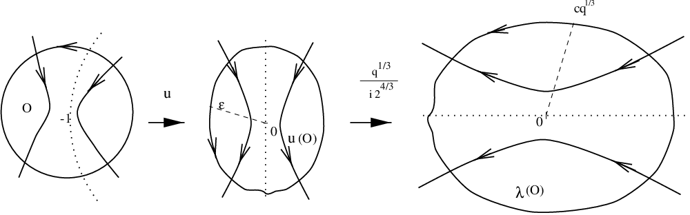
We need to devote special attention to the neighborhood of ,
where we will introduce a parametrix for the RHP,
which is related to the special solution of the Painlevé II (PII)
equation (1.4) given in Section 2.
For a discussion of parametrices in RHP’s, see e.g. [DZ2], [DKMVZ1].
Set .
The region above corresponds to .
Let be a small neighborhood of size around
, where is a fixed number which is small enough
so that first,
The goal is to solve
the RHP for explicitly in this small region.
Let in .
Figure 9.
As noted above, we choose and fix sufficiently small
(in fact, any number would do.) so that
is a bijection
from onto some open neighborhood of in the -plane :
under the bijection,
becomes a part of
the imaginary axis.
Set
Note that with fixed, there are constants
such that
(5.27)
for all .
Under the map , now becomes
part of the real axis and
(5.28)
where is a fixed small number.
As , , we see that
the contour makes an angle
and uniformly bounded away from zero as ,
hence has the general shape of the contour in
Figure 5, Section 2,
within the ball .
We define
(5.29)
and extend smoothly outside
in such a way that it is asymptotic to straight lines making angles
between 0 and with the real axis.
It is clear from the estimation in Section 2, and the
preceding calculations, that for such a contour ,
the bound (2.21) for the solution
of
(5.30)
is uniform for satisfying the relation
.
Introduce the parametrix around as follows.
Define
As , for ,
and we have for ,
(5.31)
The key fact is that is an approximation to
with error of order .
We compare, for example, the 12-components of and
on .
We focus on .
Using the variable, the -entries of and are
Let be a fixed number which is sufficiently large so
that (5.18) is satisfied.
Also let and
be fixed numbers.
As , we have the following results.
(1)
If ,
then, for some constants which may depend on ,
(2)
If ,
then,
for some constant which is independent of satisfying (5.18),
(3)
If ,
where is defined by .
6.
Let be given in Lemma 4.3,
.
Decompose where
and .
Note that on the support of the measure in (4.13),
for .
Figure 10. and
Lemma 6.1.
Define
where and the branch is chosen to
be analytic in
and for real . Then
(1)
is independent of the path in ,.
(2)
.
(3)
.
Proof.
Property (i) follows from a standard reside calculation
: the change in around
the point at is , and the change in
around is . Property (ii) follows from the definition of .
For (iii), set
for , .
From the variational condition (4.7), we have .
Differentiating,
A residue calculation similar to that in (i), now shows that .
Therefore we have .
∎
Note that for
outside the support of , i.e. for .
By (4.11) and above Lemma, our RHP becomes
We use the same conjugation (5.2)
for as in the case .
Then our new jump matrices for are
(6.2)
and .
Set
where and are open arcs as chosen below.
Note the factorization on .
Set , so that .
Recall the Cauchy-Riemann equations in polar coordinates ,
For ,
is pure imaginary and
Hence
Therefore for fixed , , there is
such that (resp. ) for with
(resp. ).
We take (resp, )
such that (resp, )
on (resp, ).
Clearly there exist such that
(resp, ), for all
(resp, ), apart from a small neighborhood
of the endpoints.
Introduce the regions ,
as in Figure 10.
Define as follows,
Then is given by
and
(6.3)
From Lemma 6.1 (iii) and the second variational
condition in (4.7), we have, for any ,
(Recall that the inequality in (4.7) is strict
from Lemma 4.3 (ii)).
Also from the choice of and ,
on , , respectively.
Therefore as ,
(6.4)
The following result can be verified by direct calculation.
Our goal now is to show that indeed
as . As in Section 5, we must control
the behavior of the solution of the RHP for near the
endpoints, where the rate of exponential convergence
, becomes smaller and smaller.
Let be fixed numbers, let
be a fixed, sufficiently small number satisfying (6.35) below,
and let be a fixed, sufficiently large number
satisfying (6.32) and (6.39) below.
We consider 3 cases for :
(1)
(2)
(3)
Calculations similar to those that are needed for the asymptotics
of the orthogonal polynomial on the real line (see, [DKMVZ1]),
show that for ,
(6.6)
The error is uniform for for any fixed .
However, we will not use this result, utilizing instead (stronger) estimates
from [Jo1] (see next section).
Figure 11.
We consider case (iii).
Set with and .
In defining above, there is some freedom in the choice
of and .
We make the following choice (see (6.11) below).
Set as ,
and let be the contour defined in Figure 6
for this specific .
Let ,
and let be small and fixed (see (6.7), (6.10) below).
For definiteness, we can, and do assume that the rays
make an angle of with the real axis.
Consider .
If is large enough, then .
Set .
We choose such that (cf. (5.25))
(6.7)
is a bijection from an open neighborhood of onto .
Clearly there are constants such that
for all .
Under , the points are mapped into respectively,
and .
Consider a point , the inverse image of
a point .
Changing variables twice,
and ,
(6.8)
where is defined to be analytic in and
positive for real ;
,
which is analytic in and ;
, which is also analytic
in and .
Since is a straight ray of angle
at , ,
which yields
(6.9)
provided is sufficiently small so that
(6.10)
for , where the terms on the LHS
are given in (6.8).
The same choice of gives rise the same
result for , and
also
for .
We thus fix by choosing
(6.11)
and extending it to a contour of the general shape
as in Figure 10.
Define
(6.12)
where solves the RHP of Painlevé II equation
given by (2.25) and (2.26).
Then solves the RHP on
in which the jump matrix is given by
In a similar manner, for such that ,
same result holds and for ,
the difference of the -entries of and satisfies
.
For ,
.
Again by (6.8),
the difference of the -entries of and satisfies
.
Therefore, we have
(6.15)
Secondly, for ,
implies
exponential decay for and
for and
, respectively.
Therefore we have
Therefore, from (6.3)
using
and the fact that is bounded for ,
(this follows, for example from (2.18) and the boundedness of
; alternatively statements like (2.28) are true also
for all the -derivatives of , etc.),
(6.20)
Finally we consider the case (ii), .
We conjugate with jump matrix given
by (6.2), as follows.
(6.21)
Define ,
where is the same as in Lemma 6.1, but
now we choose the branch so that
is analytic in , and
as .
Then the jump matrix for is given by
(6.22)
and .
Figure 12.
Noting the factorization
on ,
we define (see Figure 12)
so that
As in the case of , we have for and
for .
Therefore taking , we have
(6.23)
This RHP can be solved explicitly as in Lemma 6.2,
and we find
(6.24)
where
is now analytic in and
as .
From (6.24), we have and
as .
Again, we need to construct parametrices around and
in order to prove
that indeed .
Note that : this follows either by direct calculation
or by a general argument as .
where is the Airy function.
Then satisfies the jump conditions
(6.26)
Let and be neighborhoods
around and of size
, respectively, where is a small,
fixed number chosen to satisfy (6.27), (6.29) below.
Since ,
and have no intersection,
provided
(6.27)
For definiteness we assume that and
are oriented counterclockwise.
In , a simple substitution shows that
,
where is analytic and .
Here and
.
Define
(6.28)
where is analytic in and
as .
Of course, .
Figure 14.
It is a simple calculus question to verify that we may choose
sufficiently small so that
(6.29)
Define .
As in the construction in [DZ2], set (cf. (4.34) in [DZ2])
(6.30)
and for , define the parametrix
for by
(6.31)
Then satisfies the same jump conditions
on as ; .
And if becomes large, then
for ,
.
Therefore,
(6.32)
then by the explicit choice of in (6.30), we find
for ,
(6.33)
Noting the symmetry ,
define , and
for
set .
We now extend
to to have the same general shape as in Figure 12.
Finally, for ,
define .
Set .
Then solves a RHP on
with
the jump matrix ,
(6.34)
Let be a fixed, small number : for example, we may take
satisfying (6.7), (6.10) above.
Choose sufficiently small so that
(6.35)
for .
By calculations similar to (6.8) and (6.9),
for
(in fact the estimate is true on the full set
)
and also for
.
Thus,
for
.
Also, by calculations similar to (6.8) and (6.9) again,
for
.
Therefore we have estimation
(6.36)
Furthermore, from calculations similar to (5.23),
on ,
using on the integration contour for the second inequality,
(6.37)
The same calculations apply to the other part of
and also
to ,
so that
.
On the other hand, and
, and hence, by the
above estimates,
and
.
Thus
(6.38)
Using the choice of and , direct
calculation shows that , hence (as
), are uniformly bounded for in the region
,
for .
On the other hand, even though the contour
varies with and , the length of
is uniformly bounded for .
Also a simple scaling argument shows that the Cauchy operators on
are uniformly bounded for
.
Therefore,
Note that this is consistent with the result (6.6) for case (i)
where .
Summarizing, we have proven the following results.
Lemma 6.3.
Let be fixed numbers.
Let be a fixed sufficiently
small number satisfying (6.35),
and be a fixed, sufficiently large number
satisfying (6.32) and (6.39).
As , we have the following asymptotics.
(1)
If ,
where the error is uniform for for
any fixed .
(2)
If ,
where the error is uniform in the region.
(3)
If ,
where is defined by , .
Note that, comparing Lemma 6.3 (iii) with Lemma 5.1 (iii),
we have same result everywhere in the region ,
(6.41)
where is defined by ,
and is any fixed positive number.
where is independent of and is fixed once
satisfying (6.35) is determined.
7. Asymptotics of as
In this Section, using Lemmas 5.1 and 6.3,
we obtain the large behavior of .
In the following are fixed numbers
between and , and
are fixed and positive.
These numbers are free apart from the following requirements :
(d) satisfies (6.32), (6.39)
and condition (7.8) below.
We consider the following five cases for and :
(1)
(2)
(3)
(4)
(5)
Consider case (i).
For any , .
From Lemma 5.1 (i), we have as ,
(7.1)
Consider case (ii).
We split the sum into two pieces.
where and represent the regions
For , .
From Lemma 5.1 (ii), for some constant , independent of
satisfying (5.18),
Using the fact that
is monotone decreasing in the second inequality below,
we have, as ,
(7.2)
We use the change of variable for
the integral in the third line.
The fifth inequality is obtained from the substitution
,
and at the end, we have used .
The fourth equation is obtained using the change of variable
, and for the sixth equation,
we use the fact that
is uniformly bounded for
(see the remark below (6.19)).
To pass from the second to the third line, note that
for integers ,
(7.5)
For the case at hand, a simple calculation shows that
Also, the contribution to the integral from the interval
is .
For ,
As , by a calculation similar to the case (ii), again using
the monotonicity of
for the second inequality,
we have
The first inequality follows from Lemma 5.1 (ii) (note that,
by assumption, satisfies (5.18)).
For the second line, in order to control the contribution
to the integral from the interval
, we use the inequality
for large enough .
For the third line, we use the change of variable
, and
for the fourth line, we use the inequality
for sufficiently large .
The fifth equation is obtained from the substitution ,
and for the sixth line, we have used the inequality
for sufficiently large .
Summing up all these calculations, for
with , we have, as ,
for a constant which depends on , and for a
constant which is independent of .
Using the asymptotics of as
(see (2.17)), we have
(recall )
(7.6)
Now we consider case (iv),
.
We write
where indicate the following regions :
For , we have for sufficiently large,
.
Therefore, using (6.42), we obtain
(7.7)
The first line follows from the inequality
for ( note from (6.42) that is independent of
).
In the second line, we use the monotonicity of
and of
in the region .
In the succeeding lines, we have used the changes of variables
, and .
For the last line, note that , and we require
(7.8)
Remark : In estimating the sum in the second line of (7.7)
by an integral, the monotonicity of the integrand plays a crucial role :
we cannot, for example, use an estimate of the form (7.5), as
the derivative is not sufficiently small.
For , we have
.
Calculations similar to
the previous cases (i), (ii) and (iii) show that
The result follows by splitting the sum into the following
regions ,
and
: we leave the detail to the reader.
Therefore, for , we have
(7.9)
For case (v), we use the estimation of [Jo1] given in the
Lemma 7.1 (v) below.
Summarizing, we have
Lemma 7.1.
Let and be fixed number.
Suppose that and satisfy conditions
(a),(b),(c) and (d) given at the beginning of this Section, respectively.
Set
(7.10)
We have the following estimates for the large
behavior of :
(1)
If ,
for some constants which may depend on .
(2)
If ,
for constants C,c independent of .
(3)
If ,
so that ,
there is a constant which depends on ,
and a constant which is independent of ,
such that
The really new results in this Lemma are (iii) and (iv).
Indeed, (i) and (ii) can also be obtained from (1.19),
and as indicated, (v) is given in [Jo1].
8. De-Poissonization Lemmas
In this section, we present two Lemmas which show that is
a good approximation of .
We need a Lemma showing the monotonicity of in .
The statement and proof can be found in [Jo1].
Lemma 8.1.
For all ,
Using this monotonicity result,
the following Tauberian-like “de-Poissonization” Lemma can be proved.
This is a modification of Lemma 2.5 in [Jo1] and
the proof is the same.
Lemma 8.2.
Let be a fixed real number.
Set
and .
Then there are constants and such that
for , .
The reader will observe that the above Lemma is actually
enough for all of our future calculations.
Nevertheless, for convenience and the purpose of illustration,
we use the following Lemma for the convergence of moments.
Lemma 8.3.
There exists such that
for all sufficient large , .
Proof.
Note that . Using Lemma 8.1 and
Stirling’s formula for sufficiently large , we have from (1.11),
where .
One can easily check that is a decreasing function
for . Thus
for sufficiently large , .
For the second inequality, note that by definition.
Again, using Lemma 8.1 and
Stirling’s formula for sufficiently large ,
where .
One can check that for ,
so that .
If is sufficiently large, .
Therefore
for sufficiently large , .
∎
9. Proofs of main Theorems
In this Section, we prove the main Theorems.
Proof of Theorem 1.1
Assume for definiteness that .
For , the calculation is similar.
From the definition of ,
(9.1)
Set
As is fixed, observe that , as .
Using Lemma 8.2 with any fixed value of , we have
Set
(cf. the definition of in (7.10).)
Then, for all large ,
Let be any sufficiently large, fixed number satisfying
condition in Lemma 7.1.
Using Lemma 7.1 (iii), we have, for some constant
which depends on , and a constant which is
independent of ,
Taking , and then taking , we obtain,
For , we obtain the same limit by a similar calculation,
Thus, recalling in (2.18),
integration by parts yields
Proof of Theorem 1.2
Integrating by parts,
where
as in Theorem 1.1.
From Theorem 1.1, we have pointwise convergence of to .
We need uniform control of for large .
Let be a sufficiently large, fixed number
and be a fixed, sufficiently small number.
Set .
First consider the case when .
If , then .
For ,
(9.1) and Lemma 8.3 yield
Inserting the above estimates (9.9) and (9.11)
into (9.8), we obtain for
(9.12)
as .
Once again, as for , it follows by
the dominated convergence theorem that
(9.13)
Appendix A
As advertised in the Introduction, in
this Appendix we give a new derivation of the formula
(A.1)
where , and is the distribution function for the length,
, of the longest increasing subsequence in the random permutation
from . We set .
Let , ,
be a partition of , i.e. , , are positive integers and
; we write . With we can associate
a Young diagram, also denoted by , in the standard way, see for example
[Sa]. In the Young diagram there are boxes in the row. If we
insert the numbers in the boxes in such a way that the numbers
in every row and column are increasing we get a (standard) Young tableau
; has shape , . Let denote the number of
rows in .
Schensted, [Sc], has constructed a certain bijection, the Schensted
correspondence, between the permutation group and pairs of
Young tableaux with the same shape , where
. This correspondence has the property that if , , then equals the length, ,
of the first row in , and the length, , of the longest
decreasing subsequence in equals , the number of rows
in . For details see [Sa].
If we put the uniform probability distribution on then clearly
the random variables and have the same distribution
(just reverse the permutation). Let denote the number of Young
tableaux with shape . Then, by the Schensted correspondence,
(A.2)
If we set , , we have the following formula,
due to Frobenius and Young,
(A.3)
see for example [Si]. Note that
and . Combining the formulas (A.2)
and (A.3) we get
(A.4)
where the means that we sum over all different integers
such that , and is the
Vandermonde determinant. That we can remove the ordering of the
’s in (A.4) follows from symmetry under
permutation of . The constraint is
removed by the Poissonization
(A.5)
where
We have used the fact that and
, since the ’s are different integers. The condition that
the ’s are different can then be removed since otherwise .
Observe that is a Hankel determinant with respect to the
discrete measure
see [Sz1], i.e.
If , , are any polynomials with and leading
coefficient , row and column operations on the determinant gives
(A.6)
We now make a particular choice of , ,
if and , so that
(A.7)
The elements in the Hankel determinants can then be written
(A.8)
Now,
and hence we can perform the differentiations in (A.8) and get
where . Inserting this identity into
the formula (A.6) yields
(A.9)
where is the Toeplitz determinant
and . Hence, using the formula (A.5), we get , which is what we wanted to prove.
In the remaining part of this appendix we will give a heuristic argument
showing why we can expect the random variable to behave
like the largest eigenvalue of a random hermitian matrix. From our
considerations above we see that
By the same computations as above this leads to
(A.10)
where
Note that as . We can think
of
(A.11)
as the probability of the configuration
. This probability has
the form of a discrete Coulomb gas
on at inverse temperature
confined by an external potential. An random hermitian
matrix with a probability density of the form
has an eigenvalue density
with ; are the eigenvalues of .
Thus we can think of the ;s as some kind of “eigenvalues”.
Let
i.e. is the probability that the largest “eigenvalue”
is . Then, by (A.9) and (A.10),
(A.12)
Now, the essential contribution to the right-hand side of (A.12)
comes from
around since otherwise
is very small. Thus
i.e. is like the probability that the largest
“eigenvalue” in the discrete Coulomb gas (A.11)
is .
References
[AS]
M.Abramowitz and I.A.Stegun, Handbook of Mathematical Functions,
Dover Publications, New York, (1965).
[AD]
D.Aldous and P.Diaconis, Hammersley’s Interacting Particle
Process and Longest Increasing Subsequences,
Prob. Th. and Rel. Fields, 103, 199-213, (1995).
[Bo]
A.Borodin, Longest increasing subsequences of random
colored permutations, Electron. J. Combin., 6 (1),
R13, (1999).
[BB]
R.M.Baer and P.Brock, Natural sorting over permutation spaces,
Math. Comp., 22, 385-410, (1968).
[BC]
R.Beals and R.Coifman, Scattering and inverse scattering for
first order systems, Comm. Pure Appl. Math., 37,
39-90, (1984).
[BDJ]
J.Baik, P.Deift and K.Johansson,
On the distribution of the length of the second row
of a Young diagram under Plancherel measure,
preprint, LANL E-print math.CO/9901118.
[BR]
J.Baik and E.Rains, Symmetrized increasing subsequence problems,
in preparation.
[CG]
K.Clancey and I.Gohberg, Factorization of Matrix Functions
and Singular Integral Operators, Birkhäuser, (1981).
[De]
P.A.Deift, Integrable Hamiltonian systems. Dynamical systems
and probabilistic methods in partial differential equations, 103-138,
in Lectures in Applied Mathematics, 31, edited by
P.A.Deift, C.D.Levermore and C.E.Wayne, American
Mathematical Society, Providence, RI, 1996.
[DeZe1]
J.-D.Deuschel and O.Zeitouni, Limiting curves for i.i.d.
records, Ann. Probab., 23, 852-878, (1995).
[DeZe2]
J.-D.Deuschel and O.Zeitouni, On increasing subsequences of
i.i.d. samples, preprint, (1997).
[DIZ]
P.A.Deift, A.R.Its and X.Zhou, Long-time Asymptotics
for Integrable Nonlinear Wave Equations,
in Important Development in Soliton Theory,
2nd Edition, edited by A.S.Fokas and V.E.Zakharov,
Springer-Verlag, to be published.
[DKM]
P.A.Deift, T.Kriecherbauer and K.T-R McLaughlin,
New Results on the Equilibrium Measure for Logarithmic potentials
in the Presence of an External Field, J. Approx. Theory,
95, no.3, 388-475, (1998).
[DKMVZ1]
P.A.Deift, T.Kriecherbauer, K.T-R McLaughlin, S.Venakides
and X.Zhou, Asymptotics for Polynomials Orthogonal with
respect to Varying Exponential Weights, Internat. Math. Res.
Notices, no. 16, 759-782, (1997).
[DKMVZ2]
P.A.Deift, T.Kriecherbauer, K.T-R McLaughlin, S.Venakides
and X.Zhou, Strong Asymptotics for Orthogonal Polynomials with
respect to Varying Exponential Weights via Riemann-Hilbert
Techniques, To appear in Comm. Pure. Appl. Math.
[DKMVZ3]
P.A.Deift, T.Kriecherbauer, K.T-R McLaughlin, S.Venakides
and X.Zhou, Uniform Asymptotics for Polynomials Orthogonal with
respect to Varying Exponential Weights and Applications to
Universality Questions in Random Matrix Theory,
To appear in Comm. Pure. Appl. Math.
[DS]
P.Diaconis and M.Shahshahani, On the Eigenvalues of
Random matrices, J. Appl. Prob. 31, 49-61, (1994).
[DVZ1]
P.A.Deift, S.Venakides and X.Zhou, The collisionless shock
region for the long-time behavior of solutions of the
KdV equation, Comm. Pure Appl. Math., 47 no. 2, 199–206, (1994).
[DVZ2]
P.A.Deift, S.Venakides and X.Zhou, New Results in Small
Dispersion KdV by an Extension of the Steepest Descent Method for
Riemann-Hilbert Problems, Internat. Math. Res.
Notices, no. 6, 285-299, (1997).
[DZ1]
P.A.Deift and X.Zhou, A Steepest Descent Method for
Oscillatory Riemman-Hilbert Problems; Asymptotics for
the MKdV Equation, Ann. Math., 137, 295-368, (1993).
[DZ2]
P.A.Deift and X.Zhou, Asymptotics for the Painlevé II
Equation, Comm. Pure. Appl. Math., 48, 277-337, (1995).
[ES]
P.Erdös and G.Szekeres, A combinatorial theorem in geometry,
Compositio Math., 2, 463-470, (1935).
[FIK]
A.S.Fokas, A.R.Its and V.E.Kitaev, Discrete Painlevé
equations and their appearance in quantum gravity,
Comm. Math. Phy., 142, 313-344, (1991).
[FMZ]
A.S.Fokas, U.Mugan and X.Zhou, On the Solvability of Painlevé I, III
and V, Inverse Problems, 8, 757-785, (1992).
[FN]
H.Flaschka and A.Newell, Monodromy and spectrum preserving
deformations, I, Comm. Math. Phy., 76, no.1, 67-116, (1980).
[FZ]
A.S.Fokas and X.Zhou, On the Solvability of Painlevé II and IV,
Comm. Math. Phy., 144, 601-622, (1992).
[Ge]
I.M.Gessel, Symmetric functions and P-recursiveness,
J. Combin. Theory. Ser. A, 53, 257 - 285, (1990).
[GK]
I.Gohberg and N.Krupnik, One-Dimensional Linear Singular
Integral Equations vol.I and II, Operator theory, advances
and applications ; v. 53-54, Birkhäuser Verlag, Basel, 1992
[GW]
D.J.Gross and E.Witten, Possible third-order phase transition
in the large N lattice gauge theory, Phys. Rew. D, 21,
446-453, (1980).
[GWW]
I.M.Gessel, J.Weinstein and H.S.Wilf, Lattice walks in
and permutations with no long ascending subsequences,
Electr. J. Combin., 5(1), (1998).
[Ha]
J.M.Hammersley, A few seedlings of research, Proc. Sixth
Berkeley Symp. Math. Statist. and Probability, Vol. 1,
345-394, University of California Press, 1972.
[Hi]
M.Hisakado, Unitary matrix models and Painlevé III,
Modern Phys. Lett. A, 11, no.38, 3001-3010, (1996).
[HM]
S.P.Hastings and J.B.McLeod, A boundary value problem
associated with the second Painlevé transcendent and
the Korteweg de Vries equation, Arch. Rational Mech. Anal.
73, 31-51, (1980).
[Ka]
S.Kamvissis, On the Long Time Behavior of the Doubly Infinite
Toda Lattice under Initial Data Decaying at Infinity,
Comm. Math. Phy., 153, 479-519, (1993).
[Kn]
D.E.Knuth, The art of computer programming,
vol. 3 : sorting and searching,
2nd ed., Addison Wesley, Reading, Mass., 1973.
[IN]
A.R.Its and V.Yu.Novokshenov, The Isomonodromic Deformation
Method in the Theory of Painlevé Equations, Lecture Notes
in Math.1191, Springer-Verlag, Berlin, Heidelberg, 1986.
[Jo1]
K.Johansson, The Longest Increasing Subsequence in
a Random Permutation and a Unitary Random Matrix Model,
Math. Res. Lett., 5, no.1-2, 63-82, (1998).
[Jo2]
K.Johansson, Shape fluctuations and random matrices,
LANL E-print math.CO/9903134.
[Jo3]
K.Johansson, Transversal fluctuations for increasing subsequences
on the plane, preprint, 1999.
[JMU]
M.Jimbo, T.Miwa and K.Ueno, Monodromy preserving deformations
of linear ordinary differential equations with rational coefficients, I.
General theory and -function,
Physica D, 2, no.2, 306-352, (1981).
[Ki]
J.-H. Kim, On the longest increasing subsequence of random
permutations - a concentration result, J. Comb. Th. A, vol. 76,
148-155, (1996).
[LS]
B.F.Logan and L.A.Shepp, A variational problem
for random Young tableaux, Advances in Math., 26,
206-222, (1977).
[Me]
M.L.Mehta, Random Matrices, Second Edition, Academic Press,
San Diago, 1991.
[Ok]
A.Okounkov, Random matrices and random permutations,
preprint, 1999.
[OPWW]
A.M.Odlyzko, B.Poonen, H.Widom and H.S.Wilf, On the
distribution of longest increasing subsequences in random permutations,
unpublished manuscript.
[OR]
A.M.Odlyzko and E.M.Rains, On longest increasing subsequences
in random permutations, in preparation.
[PS]
V.Periwal and D.Shevitz, Unitary-Matrix Models as Exactly Solvable
String Theories, Phys. Rev. Lett., 64, 1326-1329, (1990).
[Ra]
E.M.Rains, Increasing subsequences and the classical groups,
Electron. J. of Combinatorics, 5(1), R12, (1998).
[Sa]
B.Sagan, The Symmetric Group : Representations, Combinatorial
Algorithms, and Symmetric Functions, WadsworthBooks/Cole,
Pacific Grove, Calif., 1991.
[Sc]
C.Schensted, Longest increasing and decreasing subsequences,
Canad. J. Math., 13, 179 - 191, (1961).
[Se1]
T.Seppäläinen, A microscopic model for the
Burgers equation and longest increasing subsequences,
Electron. J. Prob., 1, no.5, (1996)
[Se2]
T.Seppäläinen, Large deviations for increasing sequences
on the plane, Probab. Theory Related Fields, 112,
no.2, 221-244, (1998).
[Si]
B.Simon, Representations of Finite and Compact Groups,
Graduate Studies in Mathematics vol. 10, American Mathematical Society,
1996.
[ST]
E.B.Saff and V.Totik, Logarithmic Potentials with External
Fields, Springer-Verlag, New York, 1997.
[Sz1]
G.Szegö, Orthogonal Polynomials, American Mathematical
Society Colloquium Publications, Vol 23, 4th Ed, New York, 1975.
[Sz2]
G.Szegö, On Certain Hermitian Forms Associated with the
Fourier Series of a Positive Function, Comm. Seminaire Math de
l’Univ. de Lund, tome supplementaire, dedie a Marcel Riesz,
228-237, (1952) (or Gabor Szego : Collected Papers - Vol 3
(1945-1972), 270-280, Birkhäuser, 1982).
[TW1]
C.A.Tracy and H.Widom, Level-Spacing distributions
and the Airy kernel, Comm. Math. Phys., 159, 151-174, (1994).
[TW2]
C.A.Tracy and H.Widom, Random unitary matrices, permutations
and Painlevé, preprint, LANL E-print math.CO/9811154.
[Ul]
S.M.Ulam, Monte Carlo calculations in problems of
mathematical physics, in Modern Mathematics for the Engineers,
E.F.Beckenbach, ed., McGraw-Hill, 261-281, 1961.
[VK1]
A.M.Vershik and S.V.Kerov, Asymptotics of the Plancherel
measure of the symmetric group and the limiting form of Young tables,
Soviet Math. Dokl., 18, 527-531, (1977).
[VK2]
A.M.Vershik and S.V.Kerov, Asymptotic behavior of the maximum
and generic dimensions of irreducible representations of the symmetric
group,
Functional Anal. Appl., 19, no.1, 21-31, (1985).