Multi-scale linear solvers for very large systems derived from PDEs This work presented at the Fifth Copper Mountain conference on Iterative Methods, April, 1998.
Abstract
We present a novel linear solver that works well for large systems obtained from discretizing PDEs. It is robust and, for the examples we studied, the computational effort scales linearly with the number of equations. The algorithm is based on a wavelength decomposition that combines conjugate gradient, multi-scaling and iterative splitting methods into a single approach. On the surface, the algorithm is a simple preconditioned conjugate gradient with all the sophistication of the algorithm in the choice of the preconditioning matrix. The preconditioner is a very good approximate inverse of the linear operator. It is constructed from the inverse of the coarse grained linear operator and from smoothing operators that are based on an operator splitting on the fine grid. The coarse graining captures the long wavelength behavior of the inverse operator while the smoothing operator captures the short wavelength behavior. The conjugate gradient iteration accounts for the coupling between long and short wavelengths. The coarse grained operator corresponds to a lower resolution approximation to the PDEs. While the coarse grained inverse is not known explicitly, the algorithm only requires that the preconditioner can be a applied to a vector. The coarse inverse applied to a vector can be obtained as the solution of another preconditioned conjugate gradient solver that applies the same algorithm to the smaller problem. Thus, the method is naturally recursive. The recursion ends when the matrix is sufficiently small for a solution to be obtained efficiently with a standard solver. The local feedback provided by the conjugate gradient step at every level makes the algorithm very robust. In spite of the effort required for the coarse inverse, the algorithm is efficient because the increased quality of the approximate inverse greatly reduces the number of times the preconditioner needs to be evaluated. A feature of the algorithm is that the transition between coarse grids is determined dynamically by the accuracy requirement of the conjugate gradient solver at each level. Typically, later iterations on the finer scales need fewer iterations on the coarser scales and the computational effort is proportional to rather than , where is the number of equations. We have tested our solver on the porous flow equation. On a workstation we have solved problems on grids ranging in dimension over 3 orders of magnitude, from to , and found that the linear scaling holds. The algorithm works well, even when the permeability tensor has spatial variations exceeding a factor of .
keywords
multi-grid, conjugate gradient, linear solver, porous flowAMS
65F10, 65N22, 65N551 Introduction
We present a novel linear solver that works well for large systems obtained from discretizing PDEs. It is robust and for the examples we studied, the computational effort scales linearly with the number of equations. The algorithm is based on a wavelength decomposition which combines conjugate gradient, multiscaling and iterative splitting methods into a single approach. On the surface, the algorithm is a simple preconditioned conjugate gradient with all the sophistication of the algorithm in the novel choice of the preconditioning matrix. The preconditioner is an approximate inverse of the linear operator constructed from the inverse of the coarse grained linear operator and a smoothing operator based on an iterative expansion of the operator on the fine grid. To transform the coarse grained operator to the fine grid it is pre- and post-multiplied by reduction and prolongation operators. The coarse graining captures the long wavelength behavior of the inverse operator while the smoothing operator captures the short wavelength behavior. The conjugate gradient iteration accounts for the coupling between long and short wavelengths.
The coarse grained operator corresponds to a lower resolution approximation to the PDEs. While its inverse is not known explicitly, the conjugate gradient algorithm only requires that the preconditioner can be applied to a vector. The inverse is obtained as the solution of another preconditioned conjugate gradient solver that applies the same algorithm to the smaller problem. Thus, the method is naturally recursive. The recursion ends when the matrix is sufficiently small for a solution to be obtained efficiently with a standard solver.
Basing a preconditioner on the inverse of a simpler problem is akin to using an incomplete factorization. As with an incomplete factorization, our preconditioner only requires knowledge of sparse matrices. But rather than a simple forward and backward substitution used to evaluate the inverse of the product of a lower and upper triangular matrix, our preconditioner requires an iterative method. Despite the extra effort required for the coarse inverse, the algorithm is efficient because the increased quality of the approximate inverse greatly reduces the number of times the preconditioner needs to be evaluated. In the cases we studied the computational effort is dominated by the operations performed on the finest scale.
As with the multigrid method, by utilizing several scales we obtain rapid convergence of long wavelengths. In contrast to the way multigrid algorithms are typically applied, the recursive use of the conjugate gradient algorithm at each stage enforces an accurate transition from one scale to the next. In particular, the algorithm naturally accounts for the coupling between the long and short wavelengths introduced at every level of refinement. Thus, it avoids the accumulation of errors that stem from the interaction terms between the different levels. In addition, the transition between levels is determined dynamically rather than preprogrammed with a V-cycle or W-cycle. The algorithm is robust and works well without fine tuning even when the PDE is far from diagonal in Fourier space.
2 Algorithm
Let the linear system be given by
| (1) |
With a preconditioning matrix , the system to be solved is
| (2) |
Our aim is to determine a good approximate inverse of that can be used for . This reduces the condition number of the system and hence enhances the convergence rate of any iterative solver. We use a conjugate gradient algorithm since it has the advantage that convergence can greatly be enhanced even if the preconditioner fails to account for a small number of modes.
To develop an approximate inverse, we start with a standard operator splitting of the form, see for example [2],
| (3) |
We assume that and are positive and symmetric. For our algorithm, it is necessary that the inverse of applied to a vector can be evaluated efficiently and that damps out short wave lengths. The inverse is given formally by
| (4) |
The series converges when , where denotes the matrix norm. Frequently, the matrix arising from discretizing a PDE is diagonally dominated and it can be shown that standard splittings, such as Jacobi or Gauss-Seidel, do indeed satisfy the sufficient condition for the series to converge. However, as the resolution of the discretization increases typically approaches 1. Then, the convergence of the series for is very slow.
We observe the following identity
| (5) |
for any integer . This identity is easily proved by substituting (4) for on the right hand side of the equation and resumming the series. If one replaces on the right hand side of the equation with a matrix corresponding to an approximation of , then one obtains an approximate inverse better than :
| (6) |
A measure of the improvement of the inverse can be obtained from the formula
| (7) |
Consequently, . Thus, with respect to this norm, is closer to the identity than provided that . For large systems is near 1 and for to be an effective preconditioner and need to be complementary in the sense that they approximate different parts of the spectrum of . In this case, can be a much better inverse of than either or the series given in (4) truncated after terms.
Equation (6) forms the basis for a number of approximation schemes. Tatebe [5] pointed out that will be symmetric positive definite if , , and are all symmetric and positive. We note that need be only positive and not positive definite for to be a valid preconditioner for a conjugate gradient algorithm. Consequently, the coarse grained inverse can be used for even though its null space is non-empty.
2.1 Polynomial Preconditioner
The simplest choice is . In this case, corresponds to a conventional polynomial preconditioner; i.e.,the first terms of the series for in (4). At high resolution, is typically close to 1 and is a poor preconditioner. The underlying reason is that connects only neighboring grid points and consequently provides a poor approximation of at long wave lengths. This is born out by experience showing that the number of iterations grows rapidly with the dimension of the system.
2.2 Multi-Grid Preconditioner
A better choice is that advocated by Tatebe [5] which aims to account for the long wavelengths by basing the preconditioner on a single step of a multigrid algorithm. Let be a sequence of successively coarser grids, and be the reduction and prolongation operators connecting the grids and , the coarsened operator on the grid , and and the splitting of . Here corresponds to the finest mesh and to the coarsest mesh. The preconditioner can be defined recursively as
| (8) |
where . Provided that the reduction and prolongation operators are chosen such that , the approximate inverse at every level, is symmetric. On the coarsest mesh, the problem can be solved exactly. Thus, the recursion ends with . The standard multigrid algorithm uses as an approximate inverse in conjunction with a simple iterative solver. By contrast Tatebe’s algorithm uses as a preconditioner for a conjugate gradient solver.
For to be a good approximate inverse of , the splitting must be chosen such that smoothes the shorter wavelengths to complement which operates only on the longer wavelengths. Thus, the underlying rationale for the multigrid preconditioner to be a good approximate inverse is a wavelength decomposition. When the system is large enough to require many coarsening levels, two problems can arise. The first is that many iterations are needed to account for the coupling between short and long wavelengths. The second is that errors due to the coupling can accumulate at each level to such an extent that the iterative improvement to the solution saturates and the the desired tolerance can not be achieved.
2.3 Recursive Multi-Scale Conjugate Gradient
The difficulties with the multi-grid preconditioner can be overcome by defining the preconditioner in term of the exact inverse of the coarsened operator as follows
| (9) |
In effect, and the evaluation of on a vector is computed by applying the same algorithm to the coarse grained operator. Again the recursion ends by solving the problem exactly on the coarsest level. Using the exact inverse for is the best preconditioner based on a single level of scaling.
An important feature of this preconditioner is that the long and short wavelengths are coupled at each level by a conjugate gradient solver before proceeding to the next finer grid. This prevents truncation errors from the coarsening of the operator at each level from accumulating. In particular, if the coarsened operator does poorly on a few modes, which typically occurs when the coefficients of the underlying PDE are discontinuous, then these modes will be corrected by the conjugate gradient solver with only a small penalty.
The efficiency of the algorithm is due to the high quality of the approximate inverse. This results in a preconditioned matrix with a low condition number and consequently a small number of iterations for the conjugate solvers at every level. The condition number for positive symmetric matrices is the ratio of the largest to smallest eigenvalues. The coarsening increases the smaller eigenvalues associated with the long wavelengths and the iterative splitting decreases the larger eigenvalues associated with short wavelengths. Squeezing the eigenvalues together greatly decreases the condition number of the preconditioned matrix. Of course the reduced number of iterations must overcome any increase in the cost per iteration. The numerical examples below show that this is indeed the case.
The efficiency of the conjugate gradient algorithm comes from the simple recursion relations for the conjugate directions. The orthogonality of the conjugate directions is a consequence of the linearity of the preconditioner. A potential draw back of a preconditioner that depends on a linear solver is that the preconditioner is only a linear operator if the coarse grained inverse is solved accurately. In the numerical experiments described below we have found that the coarse grained inverse only need be solved to an accuracy comparable to that desired for the overall solution on the fine grid. This may be explained by following heuristic argument. Suppose the error from the inaccuracy in the coarse grained inverse is random. Then for a large problem, dimension , the component of the error along a particular vector is likely to be small. Thus the error in orthogonality for the first few iterations, , is small. If only a small number of iterations are required because of the quality of the approximate inverse then the effect of small non-linearities of the preconditioner, introduced by the recursive solvers, is negligible.
3 Implementation
To validate the algorithm we have implemented the solver in an object oriented C++ based code. The implementation is general enough to allow for an arbitrary choice of solver and an arbitrary preconditioner at every level. We have tested the code with the conjugate gradient solver using the three preconditioners described in the previous section: polynomial preconditioner, multi-grid preconditioner and the recursive multi-scale preconditioner. In addition, the implementation includes the standard multi-grid algorithm. This enabled us to compare the algorithms while using the same extension, reduction, splitting and coarsening operators.
As a test case we used the porous flow equation
| (10) |
Here, is a permeability tensor, is the pressure and is a source. We considered only a diagonal tensor and used the linear system derived from the standard 5-point stencil for the finite difference operator on a two-dimensional regular grid. In the discretization and are cell centered fields whereas the components of are face centered; from the cell centers is offset by a cell in the x-direction and is offset by a cell in the y-direction. The face centered components of the permeability field are obtained as the harmonic mean of the adjacent cell centered values. This discretization is a special case of support operator differencing [4] and results in a matrix that preserves the positivity and symmetry of the differential operator.
The discrete operator has a unique decomposition, where is diagonal, is strictly upper triangular and is strictly lower triangular. In terms of these matrices, we used two operator splitting : the symmetric Gauss-Seidel splitting for which and , and a modified Jacobi splitting with and . In contrast to the standard Jacobi splitting, the modified version is effective in damping short wavelength errors associated with the checker board modes. Though the Jacobi splitting does work with our algorithm, it is not as effective and the results presented below are for the Gauss-Seidel splitting.
We allow for both Dirichlet and Neumann boundary conditions. Each point on the boundary can be independently chosen to satisfy one or the other condition. The type of boundary condition affects the discretized field along the boundary. In addition, the value of the boundary condition enters as a source term in the boundary cells of the discretized equations. The boundary source terms are large and under coarsening scale differently then the source terms in the interior. To avoid complications from the boundary source terms, we transform to a problem with zero boundary conditions. This is accomplished by generating a smooth field that matches the boundary conditions. We then solve the problem for with zero boundary conditions but an additional source term .
The coarse grained permeability tensor is based on the transmissivities, and where and are the width and height of a grid cell. Physically these are extensive rather than intensive quantities. The transmissivity behaves like a conductance rather than a conductivity. The component is taken as
| (11) |
where the sum is over fine cells contained within a coarse cell. When a fine cell only partially overlaps a coarse cell the value of associated with the fine cell is scaled by the fraction of the height in the overlap and inversely as the fraction of the width in the overlap. A similar construction is used for (with the sums over i and j interchanged). The coarse grained operator remains diagonal. It is typically not a scalar even if on the finest grid is chosen to be scalar. This simple coarsening properly accounts for the effect of the boundary conditions on the boundary ’s. Furthermore, the form of the Laplace operator is preserved under coarsening.
It is noteworthy that the scale factor between grids is not limited to a factor of two, nor for that matter to an integer. Consequently, the number of grid points in a linear dimension does not have to be a power of the scale factor. Typically, we scaled between successive grid levels by a linear factor of 4 which reduces the dimension of the problem at each level by a factor of 16. The effective scale factor between adjacent levels may vary slightly in order to obtain an integer grid dimension.
The reduction operator is taken as the adjoint of the extension operator. For the extension operator we use the tensor product of 1-D linear interpolations. A piecewise constant interpolation works nearly as well. In contrast to the piecewise constant interpolation, a linear interpolation requires a boundary condition. For both Dirichlet and Neumann boundaries, we chose a zero slope for the boundary interpolation. While this correctly captures the Neumann condition, it introduces a small error for the Dirichlet case. However, the viability of the piecewise constant interpolation suggests that the error is small and can be neglected. Numerical experiments confirm this suggestion. For a Neumann boundary, since near the boundary can be large, a zero boundary condition is highly detrimental to the convergence of the algorithm. The fact that the zero slope interpolation condition is acceptable for both the Dirichlet and Neumann case greatly simplifies the implementation of boundary conditions that vary between Dirichlet and Neumann from cell to cell.
The degree of smoothing is related to the scale factor. Since the smoothing operator typically connects only neighboring grid points we have chosen to be the same as the scale factor. As a result the preconditioning matrix fully couples every fine grid cell. Smaller values of would require a larger number of conjugate gradient iterations for problems in which the short wavelengths dominate the solution.
Our implementation of the conjugate gradient algorithm is conventional, as outlined in [3, §2.3.1, Figure 2.5]. We base the convergence criterion on the norm of the residual rather than the norm with respect to the preconditioner. This is because applying the preconditioner is the most expensive operation in the conjugate gradient step. It is performed at the beginning of the cycle and hence is out of date when the check for convergence is made at the end of the cycle. A convergence criterion of the same type is applied on every level. The criterion for convergence on the level is
| (12) |
where is the residual, is the number of grid points, is the desired root mean squared error of the residual on the finest level, and is an adjustable parameter that allows us to tighten the error criterion on the coarser levels. The algorithm appears not to be very sensitive to the choice of . In practice we found works well. As increases the number of iteration on the fine level gradually increases, while too small a value of results in unnecessary iterations on the coarse levels.
4 Numerical Examples
We have tested our solver algorithm on several examples of the porous flow equations. The examples below use both Dirichlet and Neumann boundary conditions, typically, constant pressure on the left and on the right, and no flow on the top and bottom. We generated random log-normal permeability field with either a Gaussian auto-correlation function or a power law auto-correlation function
where is a positive definite matrix which defines cutoff lengths for the power law behavior. The variance of the permeability field is adjusted by scaling the log of the field. Similar problems have previously been used to test the conjugate gradient algorithm with a multi-grid preconditioner [1].
Our test examples include meshes varying in size by a factor of ; from to grid points. We also have varied the difficulty of the problem by increasing the variance of the permeability field to obtain a maximum to minimum permeability ratio up to . In addition, we have adjusted the error tolerance to vary the accuracy of the solution up to machine accuracy.
4.1 Base case
For a basic test case we used a power law field on a quarter of the unit square. We choose a variance of 2 with a zero mean and minimum correlation lengths of 0.016 and 0.002 oriented at 15 degrees with respect to the x-axis. The resulting permeability field contains a wide range of wavelengths. On a grid the distribution of the log of the permeability field extends over 3.5 standard deviations. Consequently, the permeability field varies from to and the ratio of its maximum to minimum value is . The flow lines for the solution superimposed on the log of the permeability field are shown in figure 1. The conjugate gradient solver on the finest level required 5 iterations to reduce the mean squared residual by a factor of . Later we show that this corresponds to 5 digits accuracy. Replacing the Neumann boundary conditions on the top and bottom with Dirichlet boundary conditions does not change the performance of the solver.
The algorithm dynamically determines its effort on every level. From the level tree shown in figure 2 it is seen that the effort on the coarsest levels diminishes as the calculation proceeds. The total number of iterations is summarized in table 1. The effort on each level is proportional to the total number of iterations on that level times the dimension of the level. It is seen from the table that the total effort is dominated by the computation on the finest level.

To set the scale, the total computational effort is equivalent to about 1600 scalar products of vectors on the finest grid. On a workstation (SUN Ultra I, 170 Mhz) or a PC (PentiumPro, 200 Mhz) the time per point is s. This time is for the solver only and does not include initialization of the permeability fields on the coarse grids. Our implementation is memory efficient. The solver requires storage for a total of 10 vectors: 3 for the matrix, one each for the pressure field, the source field, the residual and the conjugate direction, and three temporaries to evaluate the preconditioner (9) on the residual.
| Level | Grid | dimension | iterations | iterations dimension | per cent total | |
| 4 | 4 | 4 = | 16 | 119 | 1904 | 0.03 |
| 3 | 16 | 16 = | 256 | 94 | 24064 | 0.37 |
| 2 | 63 | 63 = | 3869 | 63 | 214326 | 3.29 |
| 1 | 252 | 252 = | 63504 | 20 | 1270080 | 19.48 |
| 0 | 1001 | 1001 = | 1002001 | 5 | 5010005 | 76.84 |
| total 6520379 | ||||||

Specializing the algorithm to the Laplace equation reduces the computational effort to s per point and decreases the required memory by 4 vectors. The difference in speed, as well as memory, can be attributed largely to the much more efficient coding for the simpler linear operator. It is a remarkable fact that the same preconditioned conjugate gradient algorithm works equally well for an operator with a rapidly varying permeability field as for the simple Laplace operator.
We choose this problem, which is fairly large for a workstation, as a base case because we felt it is necessary to have several levels of coarsening to assess the quality of the algorithm. With a scale factor of roughly 4, there are only 4 coarsenings for a grid. The problem we have choosen is not trivial. The polynomial preconditioner fails to converge, and so does the standard multigrid algorithm. Our implementation of Tatebe’s algorithm succeeds and will be discussed in more detail later.
Though the algorithm has not been optimized, it is relatively insensitive to the parameters characterizing the algorithm. Figure 3 shows the effect of the scale factor between grids. For scale factors between 2 and 5, the time per point varies by only 30%. A minimum time of s per point occurs with a scale factor of 3.

4.2 Scaling behavior
For high resolution, the scaling properties of the solver algorithm are critical. To test the scaling behavior we solved a series of problems on sucessively larger grids varying in dimension by 3 orders of magnitude. We found the effort per point to be independent of the size of the grid.
We started by generating a random permeability field on a unit square with a very fine grid, . Then the grid is truncated to a square subgrid by using only the subregion defined by the lower left corner and a specified upper right corner. The field corresponds to our base case and is choosen to have a variance of 2 with a mean of zero. The cutoff lengths of the correlation function on this sequence of grids remains constant (32 by 4 cells) but the variance of the permeability field increases with the size of the grid. Consequently, the problem gets harder as the size increases.
Figure 4 shows the scaling behavior on grids ranging from to . It can be seen that the number of iterations and the time per point are almost constant. This indicates that the computational effort scales linearly with the grid dimension. Despite the variable coefficients, this scaling is better than the scaling for solving the Laplace equation with fast Fourier transforms.

We have run the same problems with Tatebe’s multi-grid preconditioning algorithm. As seen in figure 5 this algorithm requires more iterations. The overall trend is linear which indicates that the computational effort scales as . This is in line with the results of Ashby & Falgout [1]. A comparison with their results is necessarily imprecise because they concentrated on 3-D problems and a parallel implementation. The larger number of iteration in Tatebe’s algorithm is partially offset by a lower cost per iteration. For the largest problems in this series, the time per point is a factor of two greater than for our algorithm. For the small problems the two algorithms are comparable in time.
In addition, we have tested the scaling behavior on a family of problems with the permeability field generated by interpolating from the very fine grid to coarser grids on the same physical domain and then rescaling to obtain the same variance. For this family of problems, the cutoff length to the auto correlation function in units of cells is proportional to the grid size. The decreasing smoothness of the discretized field, in terms of cell to cell variation, increases the difficulty of the problem for the smaller grids. Due to the changing correlation length, with this set of problems the time per point for our algorithm decreases slightly as the grid dimension increases while Tatebe’s algorithm continues to scale as . For the largest grid our algorithm is again 50% faster than Tatebe’s algorithm.
The numerical evidence suggest that our algorithm scales as . This linear scaling behavior is one of the strong points of the recursive multi-scale conjugate gradient algorithm. In fact the only algorithms robust enough to solve this class of problems are the hybrids that combine multi-scaling with conjugate gradient. The simplest representative of this hybrid class is Tatebe’s algorithm. Our algorithm is an example of the trade-off between a higher cost per iteration and a more accurate preconditioner. These examples show that this tradeoff reduces the computational time and also improve the scaling behavior compared to Tatebe’s algorithm. Because of the favorable scaling, we expect that the advantage of the recursive multi-scale conjugate gradient algorithm to increase with the problem size.

4.3 Accuracy
In order to obtain an estimate of the accuracy of our method, we first generated a test problem for which the exact solution is known. To this end we solved our base case approximately using another solver. We intentionally did not strive for high accuracy. By adding the small residual of the approximate solution to the source term of the base problem, we created a new test problem which by construction is solved exactly by the approximate pressure field of the base problem.
By varying the error tolerance of our solver we generated a sequence of solutions. For these solutions, the iteration count as a function of the accuracy is shown in figure 6. Both the root mean squared error and the maximum error are used as measures of the accuracy. We observe that the iteration count increases linearly with the log of the accuracy until the improvement of the solution is limited by machine accuracy. The linear trend indicates that each iteration reduces the error by a factor of about 11. Consequently, only a small number of iterations are needed to achieve machine accuracy. The fact that the maximum error is within a factor of 3 of the root mean squared error indicates that the solution is uniformly accurate. This is another strong point of our algorithm and is a consequence of the preconditioner acting on all length scales.

To further test the robustness of our algorithm we increased the difficulty of the base problem by increasing the variance of the permeability field. The iteration count as a function of the variance is shown in figure 7. We observe that the iteration count is almost constant. A variance of 3 results in the value of permeability field varying from minimum to maximum by a factor of . For the larger variances, round-off errors in the finite difference approximation to limits the accuracy to which the solution can be computed.
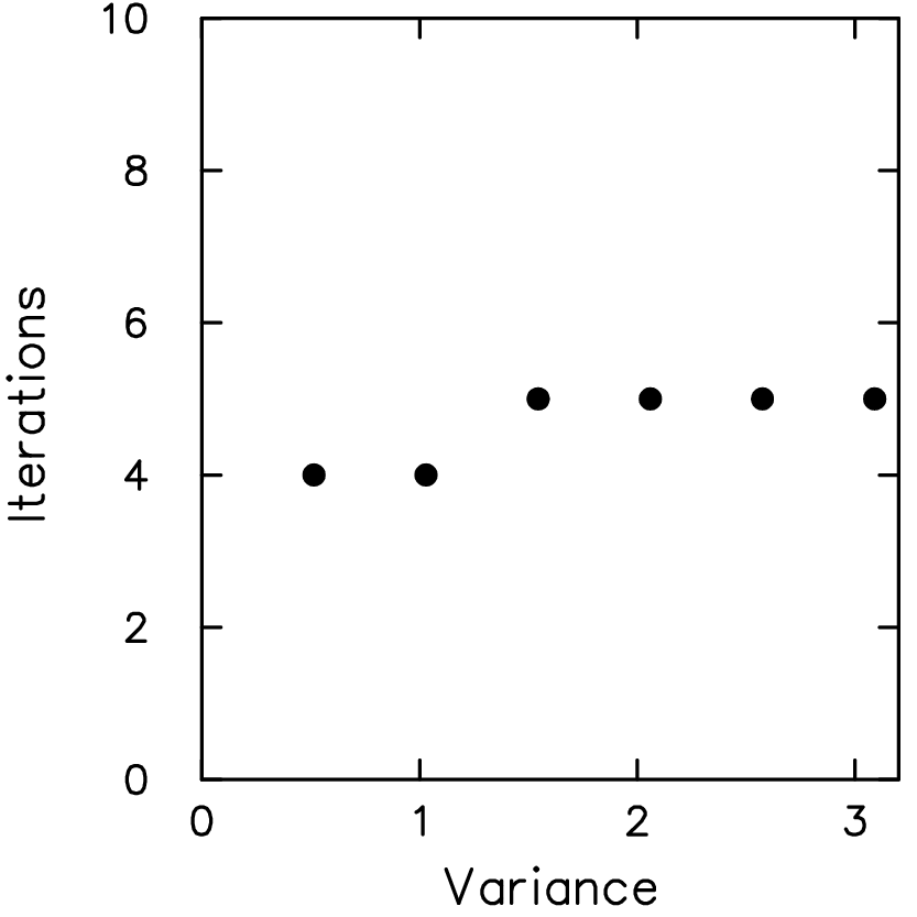
These tests shows that our algoithm is very robust. The preconditioner is effective on difficult problems. With a small increase in the number of iterations the solution can be driven to near machine accuracy. It is remarkable, that despite rather large spatial variation in the value of the permeamility field, a solution can still be obtained in only 5 iterations.
4.4 Non-isotropic permeability field
We performed preliminary tests to determine whether the algorithm can be applied to problems with large aspect ratios in either the domain or the individual grid cells. For the permeability field we used a strip of the fine field generated for the scaling study (full width and 25% of the height). The left half of the new field corresponds to the top half of the permeability field of the base case. The discretized grid of has the same overall dimension, , as the base case. In addition, as with the base case, the variance is set to 2.
We then reinterpreted the discretized field by assuming a cell aspect ratio of 10 to 1. While the initial field ranged from 0 to 1 in both the - and -directions, the new field ranges from 0 to 10 in the x-direction and from 0.25 to 0.5 in the y-direction. The rescaling results in a new permeability field in a channel with a length 40 times its width and in which the typical features (ratio of the correlation lengths) have an aspect ratio of 80 to 1.
The matrix for the problem with a 10 to 1 cell aspect ratio is equivalent to the matrix corresponding to square cells and a non-isotropic permeability field with a factor of 100 times . The flow lines superimposed on the log of the permeabilty field are shown in figure 8. The effect of the anisotropy is seen in the abrupt changes in direction of the flow lines in order to follow paths of high permeability.

We found that the solver performed better when the coarsening strategy aimed for cells with an aspect ratio of 1. Thus, despite the smaller dimension, the grid is first coarsened in the y-direction, and then uniformly in both directions. This is similar to the “semi-coarsening” strategy used for multi-grid algorithms. The iteration count on each level is shown in table 2. The finest level still required only 4 iterations but the semi-coarsening does not reduce the grid dimension by as large a factor for the first two levels and the time per point of 768s is 2.4 times as large as for the base case. We conjecture that a better coarsening algorithm which accounts for off-diagonal components of the permeability tensor would not require the semi-coarsening and that with a uniform reduction in grid size the algorithm would be as efficient as for the base case.
| Level | Grid | dimension | iterations | iterations dimension | per cent total | |
| 4 | 160 | 4 = | 640 | 1548 | 990720 | 6.3 |
| 3 | 520 | 13 = | 6760 | 191 | 1291160 | 8.2 |
| 2 | 1760 | 44 = | 77440 | 66 | 5111040 | 32.3 |
| 1 | 2000 | 147 = | 294000 | 15 | 4410000 | 27.9 |
| 0 | 2000 | 500 = | 1000000 | 4 | 4000000 | 25.3 |
| total 15802920 | ||||||
5 Conclusion
For a large system, any iterative algorithm requires an excellent preconditioner. For PDEs that can be reasonably described by discretization, a coarser discretization forms the basis for a good preconditioner. If our algorithm is well suited for the finest level of discretization, it stands to reason that it is equally well suited to the next level. Thus we are naturally led to a class of preconditioned algorithms which are recursive in nature. The preconditioner applies the very same algorithm on a coarser scale until the problem is either so coarsely resolved that further coarsening is detrimental or the problem is sufficiently small for direct solvers to be more efficient.
We have applied this philosophy to the conjugate gradient algorithm. However, it is clear that the same ideas apply to other solvers. Indeed, the high quality of the preconditioner is even more valuable for other Krylov space methods which need to store a set of conjugate directions. In our example the memory required is equivalent to 10 solution vectors on the finest grid. Since the algorithm generally converged in fewer than 10 iterations, the overhead of storing intermediate vectors would increase the memory requirement by less than a factor of 2. This suggests that similar algorithms would be effective when the operator is not symmetric or not positive definite, significantly broadening the number of problems that can be addressed. Even for porous flow problems of the type addressed here, optimum coarsening techniques would naturally lead to nonsymmetric tensors.
Our solver is yet another example that demonstrates the advantages of hybrid schemes that combine multi-grid and conjugate gradient algorithms. Because of their scaling behavior and robustness, hybrids algorithms are the only ones effective on truly large problems. Our implementation allows us to define a different preconditioner on every level. The algorithm can be specialized to a particular problem by tailoring the solver on every level to the frequency distribution of scales. From this point of view Tatebe’s algorithm and our algorithm are the end points of a large class of multi-scale algorithms. Our algorithm has the advantage of a favorable scaling, but for some problems Tatebe’s algorithm may be more suitable.
The ideas on which our approach is based are quite general and transcend the specific implementation. In many regards our implementation is a particularly simple example of the general approach. We expect in the future to see similar recursive algorithms that have equally favorable scaling behavior but can be applied to a large class of problems with more complex gridding and coarse graining schemes. In this paper we were also not concerned with parallelizing. However, it is clear that similar approaches can be parallelized and that a significant increase in speed could thus be obtained.
References
- [1] S. F. Ashby and R. D. Falgout, A parallel multigrid preconditioned conjugate gradient algorithm for groundwater flow simulations, Nuclear Science and Engineering, 124 (1996), pp. 143–159.
- [2] O. Axelsson, Iterative Solution Methods, Cambridge Univ. Press, 1994.
- [3]
R. Barrett, M. Berry, T. F. Chan, J. Demmel, J. Donato, J. Dongarra,
V. Eijkhout, R. Pozo, C. Romine, and H. Van der Vorst, Templates for
the Solution of Linear Systems: Building Blocks for Iterative Methods, 2nd
Edition, SIAM, Philadelphia, Pa., 1994.
http://www.netlib.org/linalg/html_templates/Templates.html. - [4] V. Shashkov and S. Steinberg, Support-operator finite-difference algorithm for general elliptic problems, J. Comput. Phys., 118 (1995), pp. 131–151.
- [5] O. Tatebe, The multigrid preconditioned conjugate gradient method, in Proceedings of the Sixth Copper Mountain conference on Multigrid Methods, 1993, pp. 621–634.