The honeycomb model of tensor products I:
Proof of the saturation conjectureThanks: Supported by an NSF Postdoctoral Fellowship.Thanks: Partially supported by NSF grant DMS-9706764.
Abstract.
Recently Klyachko [Kl] has given linear inequalities on triples of dominant weights of necessary for the the corresponding Littlewood-Richardson coefficient to be positive. We show that these conditions are also sufficient, which was known as the saturation conjecture. In particular this proves Horn’s conjecture from 1962, giving a recursive system of inequalities [H].
Our principal tool is a new model of the Berenstein-Zelevinsky cone for computing Littlewood-Richardson coefficients [BZ, Ze], the honeycomb model. The saturation conjecture is a corollary of our main result, which is the existence of a particularly well-behaved honeycomb associated to regular triples .
1991 Mathematics Subject Classification
Primary 05E15, 22E46; Secondary 15A421. The saturation conjecture
A very old and fundamental question about the representation theory of is the following:
For which triples of dominant weights does the tensor product of the irreducible representations with those high weights contain a -invariant vector?
Another standard, if less symmetric, formulation of the problem above replaces with its dual, and asks for which is a constituent of . In this formulation one can without essential loss of generality restrict to the case that , , and are polynomial representations, and rephrase the question in the language of Littlewood-Richardson coefficients; it asks for which triple of partitions is the Littlewood-Richardson coefficient positive.
It is not hard to prove (as we will later in this introduction) that the set of such triples is closed under addition, so forms a monoid. In this paper we prove that this monoid is saturated, i.e. that for each triple of dominant weights ,
This is of particular interest because Klyachko has recently given an answer11 1 Klyachko gives a finite set of inequalities, that as a set are necessary and sufficient for this asymptotic result. However, Chris Woodward has informed us that contrary to Klyachko’s unproven claim in [Kl], the inequalities are not independent – not all of them determine facets of the cone. This will be the subject of inquiry of our second paper [Hon2]. to the general question above, which in one direction was only asymptotic [Kl]:
If has a -invariant vector, then satisfy a certain system of linear inequalities derived from Schubert calculus (plus the evident linear equality that be in the root lattice; in the L-R context this asks that the number of boxes in the partition is the number of boxes in and together). Conversely, if satisfy these inequalities, then there exists an integer such that the tensor product has a -invariant vector.
Our saturation result completes this converse, saying that Klyachko’s inequalities completely characterize the monoid. The survey papers [F, Ze] point out another important consequence of these two results taken together: Horn’s conjecture [H] from 1962, which gives a recursive system of inequalities, since the relevant Schubert calculus questions can be cast as lower-dimensional Littlewood-Richardson questions.
The main tool in this paper is the Berenstein-Zelevinsky cone [BZ, Ze], and in particular the BZ polytope associated to the triple , in which the number of lattice points is the corresponding Littlewood-Richardson coefficient. We use a new description of the BZ cone: the honeycomb model. (The reader who is willing to grant appendix 1 does not need to absorb separately the definition of the BZ cone.) This is a special case of a general way of producing polyhedra that we dub tinkertoy models. This viewpoint gives us natural ways to interpret faces of the BZ polytope as associated to simpler tinkertoys. In addition, the Gel′fand-Cetlin system fits in this theory as associated to a -dimensional tinkertoy.
The essence of the proof is as follows. We introduce a way of indexing (real) points in the Berenstein-Zelevinsky cone by planar pictures called honeycomb diagrams; this identification is in appendix 1. This rational polyhedral cone linearly projects to the space of triples of (real) dominant weights of . By [BZ], the number of integral points (honeycomb diagrams whose vertices lie at points in the triangular lattice) in a fiber of this projection is the dimension . In order to work conveniently with honeycomb diagrams, we introduce the seemingly richer notion of a honeycomb, since honeycombs can be seen to naturally fit into a polyhedral cone. Then we prove the somewhat technical theorem 1 that honeycombs are characterized by their diagrams (whose linear structure is less apparent).
If for some large we have , then the fiber over of this linear projection contains a lattice point and is thus nonempty. By rescaling we find that the fiber over is also nonempty. So the question comes down to showing that a nonempty fiber over an integral triple necessarily contains a lattice honeycomb. Equivalently, we want a way of deforming a non-lattice honeycomb with integral “boundary conditions” to a lattice honeycomb.
We do this by maximizing a linear functional, the ‘‘weighted perimeter’’,22 2 One point easily missed is that an arbitrary choice is made in choosing this functional, making the subsequent construction non-canonical – but since we only seek an existence proof, this is not a problem. on the polytope of honeycombs with given . This picks out an extremal honeycomb,33 3 It was not a priori obvious that the lattice point we seek occurs as a vertex of the honeycomb polytope. In particular, not all the vertices are at lattice points (see figure 18). Nor was it plain that a single functional could be used to pick them out uniformly for all . These facts are side consequences of the proof. the “largest lift”, which we prove in theorem 2 to have very nice properties if the three weights are suitably generic. This theorem seems to be the useful one for studying honeycombs, and will play an equally important role in the next paper in this series [Hon2].
It is then straightforward to prove from its nice properties that the largest lift is integral. A continuity argument handles the case of nongeneric triples of weights. This ends the proof.
Not all of the framework presented in this paper is strictly necessary if one only wishes to prove the saturation conjecture. In the very nice paper [Bu] a streamlined version of our proof is presented, avoiding honeycombs in favor of the hive model44 4 The first version of this paper required the reader to absorb both models and switched viewpoint back and forth. The paper [Bu] was inspired by that version, and took the approach of eliminating honeycombs, rather than hives as is done here. (presented in appendix 2), and in particular not requiring theorem 1. However, one consequence of theorem 1 is that honeycombs have a very important operation called overlaying which will be central for developments in later papers. In the next in this series we will use the overlaying operation to study which of Klyachko’s inequalities are in fact essential [Hon2].
We thank Chris Woodward for pointing out that the saturation conjecture gives a new proof of the weak PRV conjecture for , which states that (for in the positive Weyl chamber) is a constituent of . (This “conjecture” is nowadays known to be true for all Lie groups [KMP].) In fact one can do better, and without using saturation; in section 4 there is a canonical honeycomb witnessing each instance of the long-proven “conjecture”, constructed by overlaying -honeycombs.
We mention very briefly some connections to algebraic and symplectic geometry (much more can be found in [F, Ze]). By Borel-Weil, the space is the space of invariant sections of the line bundle on the product of three flag manifolds. Given two nonzero invariant sections, one of the line bundle and one of the , we can tensor them together to get an invariant section of the line bundle. The geometrical fact that the flag manifold (hence the product) is reduced and irreducible guarantees that this tensor product section is again nonzero; this is why the set of triples with invariant sections forms a monoid.
This same data is involved in defining a geometric invariant theory quotient of the product of three flag manifolds by the diagonal action of . The space is the th graded piece of the coordinate ring of this quotient space. (Klyachko’s paper is a study of the semistability conditions that arise in performing this quotient.) The BZ counting result then says that this moduli space of triples of flags has the same Hilbert function as a certain toric variety, and our saturation result says that the (by definition ample) line bundle on this moduli space actually has sections. W. Fulton has shown us examples in which this line bundle is not very ample. If one had an explicit degeneration of the moduli space to the toric variety, one might be able to relate this non-very-amplitude to the existence of nonintegral vertices on the corresponding polytope of honeycombs.
The symplectic geometry connection then comes from the “GIT quotients are symplectic quotients” theorem [MFK, chapter 8] (whose proof is essentially repeated in Klyachko’s paper, in this special case). In this case, the corresponding symplectic quotient is the space of triples of Hermitian matrices with spectra , , and which sum to zero, modulo the diagonal action of .
In particular, this identification shows directly that the existence of a -invariant vector in implies the existence of a triple of Hermitian matrices with zero sum. The reverse implication exactly amounts to the saturation conjecture.
B. Sturmfels has pointed out that the “largest lift” construction can be interpreted as selecting a vertex of the fiber polytope [BS] of the projection from the cone of honeycombs to the cone of triples of dominant weights. Combining this idea with the hypothetical degeneration of the moduli space to the BZ toric variety, this suggests that we might be able to alternately interpret the largest lift as picking out a point in the Chow quotient [KSZ] of the product of three flag manifolds by the diagonal action of .
We thank Anders Buch, Bill Fulton, Bernd Sturmfels, Greg Warrington, and Andrei Zelevinsky for careful readings and many cogent suggestions; Bill we thank especially for correcting us on a number of historical inaccuracies in the early versions.
We encourage the reader to get a feeling for honeycombs by playing with the honeycomb Java applet at
http://www.alumni.caltech.edu/˜allenk/java/honeycombs.html.
2. Tinkertoys and the honeycomb model
We fix first a few standard notations.
A weight of is a list of integers, and is dominant if the list is weakly decreasing. So ’s root lattice is the hyperplane of lists whose sum is zero.
The “graphs” in this paper are rather nonstandard; for us, a directed graph is a quadruple where the and maps from the edges to the vertices may be only partially defined – the edges may be semi- or even fully infinite. In particular, any subset of the vertices and edges gives a subgraph, where the domains of definition of the and maps are restricted to those edges that have their heads or tails in the subgraph.
For a real vector space, let denote the space of rays coming from the origin. Each ray is in a unique line . Topologically is a sphere, .
2.1. Tinkertoys.
We define a tinkertoy as a triple consisting of a vector space , a directed graph (possibly with some zero- or one-ended edges), and a map assigning to each edge a “direction” in the sphere.55 5 A related, though much more restrictive, definition has recently appeared in [GZ], in a context quite related to the polytope tinkertoys in example 1 following. In both cases, it is sort of unnatural to fix an orientation on the graph – really it is the “orientation times the direction” that comes into play.
Example 1.
Polytope tinkertoys. Any polytope in gives a natural tinkertoy, just from the vertices, the edges (oriented arbitrarily), and their directions . For example, each rectangle in with edges aligned with the coordinate axes gives us the same polytope tinkertoy (up to isomorphism).
We define a configuration of a tinkertoy as a function assigning a point of to each vertex, such that for each two-ended edge
More generally, we say is a virtual configuration of if for each two-ended edge
The set of virtual configurations is a linear subspace of the vector space of all maps . The set of configurations is a closed polyhedral cone in this subspace, cut out by the conditions that that the edges be of nonnegative length; we call it the configuration space or cone of configurations of the tinkertoy . We can use the vector space structure to define the sum of two (virtual) configurations.
If is endowed with a lattice, one can speak of lattice configurations of the tinkertoy: these are the ones such that the map takes to lattice points in .
Example 2.
Configurations of polytope tinkertoys (for cognoscenti of toric varieties only – we neither use nor prove the statements in this example). In the case a convex lattice polytope such that the edges from each vertex give a -basis of the lattice, there is an associated smooth toric variety, and the polytope tinkertoy is just a way of encoding the (complete) fan of the polytope. The vector space of virtual configurations of the corresponding polytope tinkertoy can be naturally identified with the second equivariant cohomology group of the toric variety [GZ]; the cone of actual configurations is then identified with the equivariant Kähler cone, and the lattice configurations with the equivariant Chern classes of nef line bundles.66 6 In order to model line bundles on noncompact toric varieties using tinkertoys, we would need a more ornate definition of tinkertoy including higher-dimensional objects than edges, and also a more ornate definition of configuration, assigning affine subspaces to all objects in the tinkertoy (not just to the vertices). These additional complications only serve to obscure the simplicity of the tinkertoys actually used in this paper.
We define a subtinkertoy as a tinkertoy living in the same space , with any subgraph , and the same assigned directions (restricted to the subset ). We will not have much need for morphisms of tinkertoys, but we do define an isomorphism between two tinkertoys in the same space as a correspondence between the two graphs, intertwining the direction maps .
Example 3.
The Gel′fand-Cetlin tinkertoy. Let , for , and consist of two groups of edges , each . Every edge is assigned the direction .
One important subtinkertoy in this consists of the “primary” vertices and no edges. The configurations of the Gel′fand-Cetlin tinkertoy restricting to a given configuration of the primary vertices form a polytope called the Gel′fand-Cetlin polytope. Each high weight of gives a (weakly decreasing) list of integers, which we take as a lattice configuration of the primary vertices. The lattice points in the Gel′fand-Cetlin polytope are called Gel′fand-Cetlin patterns, and they count the dimension of the corresponding irreducible representation of . Note that not every configuration of the primary vertices can be extended to a configuration of the whole Gel′fand-Cetlin tinkertoy – for this to be possible, the coordinates of the primary vertices must be weakly decreasing.
Return now to the general case. If the two-ended edges of a tinkertoy are all of positive length in a configuration , or equivalently
we call the configuration nondegenerate.77 7 One last toric variety remark: in the context of the configurations of polytope tinkertoys, nondegenerate lattice configurations correspond to ample line bundles on the corresponding projective toric variety. Otherwise we say that is a degenerate configuration, each edge with is a degenerate edge of , and each vertex attached to a degenerate edge is a degenerate vertex of . Note that not every tinkertoy has a nondegenerate configuration – for example, make a tinkertoy with vertices and two edges from to with different given directions .
The following proposition is of a type standard in convex geometry:
Proposition 1.
If a tinkertoy has a nondegenerate configuration, then the nondegenerate configurations form the interior of the cone of configurations, and every configuration is a limit of nondegenerate ones. If doesn’t have any nondegenerate configurations, there is some edge that is degenerate in every configuration of .
It is worth noting that if is a degenerate configuration of a tinkertoy , one can associate a smaller tinkertoy in which all the degenerate edges of have been removed, and any two vertices connected by a series of degenerate edges have been identified; the configuration then descends to a nondegenerate configuration of this smaller tinkertoy. In this way each face of the cone of configurations can be identified with the full cone of configurations of a smaller tinkertoy.
2.2. The relevant vector space for this paper’s tinkertoys.
From here on out, all our tinkertoys are going to live in the same space , a plane containing the triangular lattice . This plane has three coordinate directions , and each direction will be one of these.
In particular, as one traverses the interval assigned to an edge by a configuration, one coordinate remains constant while the other two trade off, maintaining zero sum. We will call this the constant coordinate of the edge in the configuration.
Example 4.
The honeycomb tinkertoy, in figure 1. (This case is too small to see why these are named “honeycombs”.) This tinkertoy has one vertex which is the tail of three edges in the three coordinate directions, three vertices that are each the head of three such edges, for a total of four vertices and nine edges (six of which have no tails and are thus semiinfinite).
The constant coordinates on the six semiinfinite edges determine the configuration, and looking at the central vertex, we see that their sum must be zero. This equality is only sufficient for the existence of a virtual configuration: any actual configuration will satisfy also the triangle inequalities on the separations between the pairs of semiinfinite edges going going in a coordinate direction.
There is a concise way to describe the set of integral coordinates that arise in configurations of the honeycomb tinkertoy: they are exactly those such that the tensor product of the corresponding representations of contains an invariant vector. (Proof sketch: the requirement that the sum be zero is equivalent to asking that the center of act trivially on the tensor product. Then the triangle inequalities are familiar from theory.) In these cases, the configuration is unique, and so too is the invariant vector (up to scale).
Much of the rest of this section is about generalizing this example to general , which quite amazingly can also be performed in the plane .
2.3. The infinite honeycomb tinkertoy, and honeycomb tinkertoys.
As promised, . Let be the set of points88 8 This is ’s weight lattice minus its root lattice. Presumably there is a deep meaning to this – perhaps relating to the web diagrams in [Ku] – but we did not uncover it.
For each vertex such that , put on three outwardly directed edges, ending at the vertices . These will be the vertices and edges of a directed graph , in which every edge is two-ended, and each vertex has three attached edges, either all in or all out (depending on ).

The infinite honeycomb tinkertoy is then , where the direction of an edge is its direction , and the inclusion map defines a nondegenerate configuration of this tinkertoy.
The honeycomb tinkertoy is the subtinkertoy of the infinite honeycomb tinkertoy whose vertices are the contained in the triangle (automatically in the interior), and all their attached edges. This tinkertoy has tailless edges; we will call these the boundary edges of this tinkertoy. The example can be seen in figure 3.
There is a more general notion of honeycomb tinkertoy that we defer until section 3.
We call a configuration of a honeycomb or -honeycomb. It is important to distinguish the ontological levels here – the honeycomb tinkertoy is an abstract graph with some labeling by directions, whereas a honeycomb is the additional data of an actual configuration of that tinkertoy in .
Given a -honeycomb , we can read off the constant coordinates on the semiinfinite edges starting from the southwest and proceeding clockwise.99 9 If our notion of “configuration” of a tinkertoy explicitly assigned lines in to edges in , not just to those with a head or tail, we could regard this as the restriction of a configuration of the honeycomb tinkertoy to the subtinkertoy consisting of the boundary edges and no vertices. Denote these , , , as in figure 4; these are the boundary conditions of the honeycomb.
Let denote the cone of -honeycombs, and the cone of possible boundary conditions of -honeycombs. That is to say, is the image in of the map its boundary conditions .
Our purpose in introducing honeycombs is to calculate Littlewood-Richardson coefficients, the dimensions . We do this by linearly relating -honeycombs to Berenstein-Zelevinsky patterns1010 10 Gleizer and Postnikov have recently given a way of relating honeycomb configurations to Berenstein-Zelevinsky patterns that is very different from ours [GP]. in an appendix, where we establish the -linear equivalence of the Berenstein-Zelevinsky cone with the space .
That equivalence has the following consequence:
Theorem (from appendix 1).
Let be a triple of dominant weights of , and the honeycomb tinkertoy. Then the number of lattice -honeycombs whose semiinfinite edges have constant coordinates as in figure 4 is the Littlewood-Richardson coefficient .
This generalizes the case we did before as example 4.
Example 5.
In figure 5 we calculate the tensor square of the adjoint representation of . The corresponding Littlewood-Richardson rule calculation, throwing away partitions with more than three rows, gives
(Recall that to turn the -symmetric honeycomb formulation back into a tensor product decomposition, one must reverse and negate the weight considered the “output”.)

One elementary consequence of this theorem is that the sum of the constant coordinates on the boundary edges is zero. Proof: by linearity and continuity, it is enough to check on lattice -honeycombs. On the representation theory side, the sum of the constant coordinates gives the weight of the action of the center of , which must be trivial for there to be any invariant vectors. QED. We now set up a more direct proof by a sort of Green’s theorem argument, proving some other results in tandem.
For an edge in the honeycomb tinkertoy , let the closed interval be defined by
where if or is undefined the corresponding term is omitted. (Note that has no zero-ended edges, so this intersection is never over the empty set.) Say that a curve in intersects the configuration transversely if contains no points , and intersects each interval transversely or not at all.
Lemma 1.
Let be the honeycomb tinkertoy,1111 11 This lemma applies word-for-word to the more general honeycomb tinkertoys defined in the next section. a -honeycomb, and a piecewise-linear Jordan curve in intersecting transversely. For each edge let be the number of times pokes through from the inside to the outside, minus the number from the outside to the inside (the total1212 12 This is also equal to the “number of heads of landing inside minus the number of tails” – a perhaps misleading phrase, since each number is only ever zero or one! will be , , or ).
1. The sum over of the unit vectors in the directions , weighted by , is the zero vector.
2. The sum over of the constant coordinates on , weighted by , is zero.
Proof.
Since has its standard configuration, which is nondegenerate, by proposition 1 the nondegenerate -honeycombs are open dense in the cone of all -honeycombs. The space of -honeycombs intersecting transversely is open in the space of all -honeycombs, and each of the functionals above is obviously piecewise linear (and continuous) on it. Therefore the nondegenerate -honeycombs are open dense in the ones intersecting transversely, and by continuity it suffices to check the lemma for them.
If encloses one (or no) vertices the statement is easily checked. Otherwise we can connect two points on by a path within the interior intersecting transversely and separating the vertices into two smaller groups (see figure 6). This shortcut gives us two new Jordan curves, and . One checks that each of the above functionals satisfies . By induction the two terms on the right-hand side are zero, and therefore the left is also.

∎
In particular, if we take our Jordan curve to be (a PL approximation to) a very big circle, we recover the previous result that the sum of the constant coordinates on the boundary edges is zero.
2.4. Eliding simple degeneracies.
Recall from above that we call a tinkertoy configuration degenerate if some edge has length zero. This can be regarded as a configuration of a simpler tinkertoy , in which the two vertices collapsed together have been identified (and the edge removed). The configuration map descends to give a configuration of . In this way the faces of a configuration cone can be identified with configuration cones of simpler tinkertoys.
The case of interest to us is when a single edge of a honeycomb tinkertoy degenerates to a point – or more generally, when no two degenerate edges share a vertex. In this very special case there is an even simpler tinkertoy to consider, where these five edges and two vertices are not replaced by four edges and one vertex , but two edges and no vertices at all. (In particular, though ’s head/’s tail is removed, the identified edge gets the head and tail ; similarly the head and tail .)
![[Uncaptioned image]](9807160v4/blowdegenlabel.png)
We will call this modification of a tinkertoy eliding the edge , or the vertices , or just eliding the singularity. A tinkertoy created by eliding a number of edges in a honeycomb tinkertoy we call a post-elision tinkertoy. Note that there is no analogue of this for a degenerate edge in a general tinkertoy – it is crucial that so that the map is well-defined on the post-elision tinkertoy. Note also that worse degenerations, as occur in the tensor product calculation in figure 5, do not usually allow the vertex to be removed.
We will say a honeycomb has only simple degeneracies if no two degenerate edges meet in a vertex. In this case we will typically elide the degenerate edges in the sense of the paragraph above.
It is not readily apparent what the degrees of freedom of a tinkertoy are. However, for post-elision tinkertoys one can say something useful.
Lemma 2.
Let be the honeycomb tinkertoy.1313 13 Again, this lemma extends word-for-word to the general honeycomb tinkertoys defined later. Let be a -honeycomb some of whose degeneracies are simple, and be a post-elision tinkertoy obtained by eliding some of ’s simple degeneracies, so descends to a configuration of . Let be a loop (undirected) in the underlying graph of containing only nondegenerate vertices of (necessarily trivalent). Then there is a one-dimensional family of configurations of , starting from , in which one moves only the vertices in .
Proof.
We can assume that the loop doesn’t repeat vertices; if it does, it will have subloops that do not (in which case we will move a proper subset of ’s vertices).
Orient the loop, and label the vertices with signs based on whether the loop turns left or right at the vertex, as in figure 7. Because of the angles, if all the left-turn vertices move so as to shrink their non-loop edges by a fixed length , whereas the right-turn vertices move so as to extend their outgoing edge by the same , the angles remain unchanged – i.e. we have a new configuration.

∎
Note that no loop can go through semiinfinite edges. So in this previous lemma we’re only studying degrees of freedom which leave the semiinfinite edges in place. Also, because we can orient the loop either way, the loop can breathe both in and out.
3. The diagram and degeneracy graph of a honeycomb, and reconstructing a honeycomb from its diagram
3.1. Honeycomb tinkertoys and honeycomb diagrams.
For a configuration of a tinkertoy , define the diagram of the configuration to be a measure on , the sum
This is a little more information than the set-theoretic union , in that it remembers multiplicities when edges are directly overlaid. Note that we can recover the union from , as its support .
In this section we will prove that a -honeycomb is reconstructible from its diagram. There is a stronger statement – that every measure on that looks enough like the diagram of a honeycomb is indeed the diagram of a unique honeycomb (up to a trivial equivalence) – but it requires a more general definition of honeycomb tinkertoy than the honeycomb tinkertoys we have met so far.
Define a hexagon in the infinite honeycomb tinkertoy as the six vertices around a hole, i.e. a 6-tuple of vertices where divides .
Define a honeycomb tinkertoy as a subtinkertoy of the infinite honeycomb tinkertoy satisfying five conditions:
- (1)
is finite
- (2)
(the underlying graph of) is connected
- (3)
each vertex in has all three of its edges (which may now be one-ended)
- (4)
contains a vertex (it’s not just a single no-ended edge)
- (5)
if four vertices of a hexagon are in , all six are.
(It is slightly unfortunate to rule out the infinite honeycomb tinkertoy itself, but it would be more unfortunate to have to say “finite honeycomb tinkertoy” throughout the paper.) We will call the configuration of restricted from the defining configuration of the infinite honeycomb tinkertoy the standard configuration of .

A honeycomb tinkertoy has a number of semiinfinite edges in each of the three coordinate directions and their negatives. Call this ordered 6-tuple, counted clockwise from North, the type of the honeycomb tinkertoy. One fact we prove later, in lemma 6, is that any two honeycomb tinkertoys of the same type are isomorphic – that the honeycomb tinkertoys presented in figure 8 essentially capture all the types. (In fact they are better than ‘isomorphic’; they differ only by translation within the infinite honeycomb tinkertoy.) We give the more axiomatic definition above to make it easy to check, in lemma 7, that a certain subtinkertoy is itself a honeycomb tinkertoy.
If is a honeycomb tinkertoy, we define a -honeycomb to be a configuration of , and will speak of ’s type (meaning the type of ). Just as in the case of the honeycomb tinkertoy , we use to denote the cone of -honeycombs, and to denote the cone of possible constant coordinates on the set of one-ended edges of .
It is quite easy to describe the local structure of the diagram of a (perhaps degenerate) honeycomb . In the pictures to follow of honeycomb diagrams we label edges with their multiplicities (multiple of Lebesgue measure on the line).
Lemma 3.
Let be the diagram of a honeycomb . Each point has a neighborhood in which satisfies one of the following:
- (1)
- (2)
is equal to a natural times Lebesgue measure on a coordinate line through
- (3)
matches one of the following, up to rotation (here the edge multiplicities are naturals):

Figure 9. The Y, crossing, rake, -valent, and -valent vertices.
There are only finitely many points in the third class, the vertices of the honeycomb diagram . If one thinks of each of the edges meeting a vertex as pulling on the vertex with a tension equal to its multiplicity, these are exactly the ways for the vertex to experience zero total force.
Proof.
That the pictures above are the only possibilities, and the finiteness of the number of points in the third class, each follow from the finiteness of the edge set of a honeycomb tinkertoy (so the neighborhood can be shrunk to avoid the not actually meeting the point ), and the directions being multiples of from North. It remains to be sure the multiplicities are constrained as claimed.
By lemma 1, the sum of the unit outgoing edges of a vertex (weighted by their multiplicities) must be zero. So if both a direction and its negative appear with positive multiplicity, we can subtract one from each and continue. Eventually we must get to a vertex of the first type, Y, or nothing at all. ∎
Each of the points of the third class in the above we will call a vertex of the diagram .
To see that each of these vertex types actually occurs, start with the honeycombs in figure 8 (or larger versions with more hexagons) and degenerate all the two-ended edges to points. As we will show in this section, collapsing the honeycombs in figure 8 is essentially the only way to produce the singular vertices in lemma 9.
3.2. The dual graph of a honeycomb tinkertoy .
Call the lattice the root lattice (in that it is the root lattice of ), and define the root lattice triangle around a vertex of the infinite honeycomb tinkertoy to be the three points of the root lattice at -distance 2 from (these are the three closest points). We will need the small triangular graph made from a root lattice triangle, and also the region enclosed.
Fix a honeycomb tinkertoy . Define , the dual graph of , to be the union of the root lattice triangles around the vertices in – this has one vertex in each region in the standard configuration of (including the unbounded ones), with an edge connecting two -vertices if the corresponding -regions share an edge. (In this way edges in correspond to perpendicular edges in .) In particular is naturally embedded in – it has more structure than just the abstract dual graph.

Lemma 4.
Let be a honeycomb tinkertoy. Then the region bounded by its dual graph is convex, and is thus characterized (up to translation) by its 6-tuple of edge-lengths. Conversely, every convex union of root lattice triangles arises as a .
Proof.
Each vertex in gives us three vertices in (by either adding 1 to, or subtracting 1 from, each of the three coordinates), and thus a small triangle. Two connected vertices in share two of these three vertices, so their corresponding triangles in intersect in an edge (and not just a vertex).
Since is by assumption connected, any two of these triangles are connected by a chain of triangles sharing common edges. This shows that bounds a single region, not a disconnected set, nor two regions intersecting in only a vertex.
It remains to prove this region is convex. If not, it has an internal angle of more than going around some boundary vertex. This would mean four successive triangles out of the same vertex are in . On the side, that means four successive vertices around a hexagon are in . But that forces the whole hexagon to be in . So the vertex was not actually on the boundary, a contradiction. This establishes the convexity of .
The converse is simple: given a convex union of root lattice triangles we wish to realize as a dual graph , take to be the subtinkertoy of the infinite honeycomb tinkertoy lying within (those vertices, and all their edges). This is easily seen to be a honeycomb tinkertoy whose dual graph is . ∎
So the external angles are restricted to and . To rotate once, the total of the external angles must be , so there are five types, depending on the number and ordering of the two kinds of angles; see figure 11.

Not any -tuple of edge-lengths will do; the boundary of must be a closed curve. This gives two linear conditions that exactly match the zero-tension property of lemma 3. So we’ve essentially classified the possible .
To get an equally good hold of , we need a lemma saying we can reconstruct from . That will follow from a study of the length-minimizing paths connecting two points in a honeycomb tinkertoy, which we dub geodesics. (Note that there are a typically a great many paths with this minimum length.)
The following lemma says that is “geodesically convex” inside the infinite honeycomb tinkertoy.
Lemma 5.
Let be a honeycomb tinkertoy, two vertices of , and a geodesic between and in the infinite honeycomb tinkertoy. Then the vertices of are in .
Proof.
We induct on the length of , assuming that the lemma is proven for all and with geodesics shorter than .
Since is connected, and are connected under some path in . Let be the collection of hexagons enclosed by the concatenation . We can assume the cardinality of is minimal among all possible paths in that connect and . If is empty, we are done, so suppose for contradiction that is non-empty.
If is not a Jordan curve, we can break it into smaller pieces and use the induction and minimality hypotheses. Hence we may assume is Jordan.
The curve cannot contain three consecutive edges of a hexagon in ; if it did, then by property 4 required of honeycomb tinkertoys, all the vertices of this hexagon would be in . Then we could “flip” to go around the other side of the hexagon, which would remove that hexagon from and contradict the minimality assumption. Thus we may assume that does not contain three consecutive edges of any hexagon in .
To finish the contradiction we shall invoke
Sublemma 1.
Suppose is a Jordan curve whose interior is a nonempty collection of hexagons. Suppose further that does not contain three consecutive edges of a hexagon in . Then is longer than .
Proof.
Suppose for contradiction that there was a counterexample to this sublemma. We may assume that this counterexample has a minimal number of hexagons in . We may assume that contains more than one hexagon, since the sublemma is clearly true otherwise.
From hypothesis, does not contain three consecutive edges of any hexagon in . We now claim that also does not contain three consecutive edges of any hexagon in . For, if did contain three such edges, one could then “flip” these edges across the hexagon; this would preserve the length of and therefore contradict the minimality of . (If the flip operation causes to cease being Jordan, eliminate redundant edges and divide into connected components).
Now traverse once in a counter-clockwise direction, so that is always to the left. At every vertex one turns 60 degrees in a clockwise or counterclockwise direction. From the above considerations we see that one cannot execute two consecutive counter-clockwise turns while staying in the interior of , since this would imply that contains three consecutive edges of a hexagon in . Similarly one cannot execute two consecutive counter-clockwise turns while staying in the interior of . Thus, with at most four exceptions, every counter-clockwise turn in is immediately followed by a clockwise turn. But this contradicts the fact that we must turn 360 degrees counterclockwise as we traverse . ∎
Since was assumed to be a geodesic, we have the desired contradiction. ∎
Lemma 6.
One can reconstruct a honeycomb tinkertoy from its dual graph : its vertices are
The number of semiinfinite edges of in a particular direction is equal to the length of the corresponding edge of . In particular, honeycomb tinkertoys are characterized (up to translation in the infinite honeycomb tinkertoy) by their type.
Proof.
Each point in is in the set above, tautologically – a point in leads to the three points in , which lead back to the same point being in the set above.
Now fix a triangle in ; we wish to show that the center of that triangle is necessarily in . From a vertex in one can infer that at least one of the six neighboring points in is in . For example, the presence of the dotted (North) vertex in figure 12 says that up to left-right reflection, there must be a vertex in one of the regions labeled , , or .

If there’s a vertex in region , we’re done. If there’s a vertex in region or , and another vertex producing the existence of the Southeast vertex of , we can find (in figure 13) a geodesic in the infinite honeycomb connecting the two that goes through the center. Then by lemma 5 about such geodesics, the center is necessarily a vertex of .

The remaining case occurs when the only vertex can be found in region , in all three rotations of the diagram. But then by connecting two of those vertices with geodesics we find vertices in regions and , reducing to the previous case. ∎
3.3. The degeneracy graph of a honeycomb .
Fix a honeycomb tinkertoy , and its dual graph. For a -honeycomb, let be the subgraph of with the same vertex set but an edge between two vertices only if the corresponding (perpendicular) edge of is nonzero. This we will call the degeneracy graph of the honeycomb (and is also embedded in ).

Our goal is to classify the regions in , and establish that they correspond to vertices in the diagram of , thereby classifying the possible vertices in the diagram and their preimages under (á la figure 8).
Lemma 7.
The regions in the degeneracy graph of a honeycomb are convex.
Proof.
Fix a region in , and choose a vertex of which lies in the closure of . Then its image is in the support of the diagram of .
Consider the subtinkertoy of consisting of those vertices in which map to under , together with their associated edges. Let be the connected component1414 14 Actually, we shall see in the next lemma that the tinkertoy necessarily has only one connected component. of this tinkertoy that contains . Then is a honeycomb tinkertoy in its own right: the only non-trivial observation required is that if four vertices of a hexagon map to , then all six vertices must map to .
Chasing down the definitions we see that the region bounded by is just . The claim then follows from lemma 4. ∎
Lemma 8.
The regions in the degeneracy graph of a honeycomb correspond to the vertices in the diagram of .
Proof.
One direction is clear: if two vertices in give root lattice triangles in the same region of , those vertices are connected by a series of degenerate edges in , and therefore have collapsed to the same vertex of the diagram of . So for each region in , we can speak of ’s -vertex. The converse is more difficult; we must show that two distinct regions and in give vertices in the diagram of that are physically separated.
One case is easy. If and are adjoining regions, then the existence of the edge in separating them says that the corresponding edge in is nonzero. But this is exactly the displacement between ’s -vertex and ’s -vertex, so they are in different places, as desired. For nonadjoining and we will have to add together a bunch of such nonzero displacements and hope to get a nonzero sum.
Let be a generic point in , and a generic point in , and let the straight-line path connecting them. Then does not intersect the vertices of and only intersects the edges of transversely.

We can now compute the vector in separating the points in corresponding to the regions and . Each time crosses a wall – an edge still left in – there is an associated nonzero displacement, the vector difference of the -vertices of the regions on the two sides of the wall. Adding up all these displacements we get the total vector difference we seek, the displacement of the vertices corresponding to and . (It is worth emphasizing that this gives a path in itself, as indicated in figure 15.) But note now that each individual term has positive dot product with the vector , since it is perpendicular to the wall that has just crossed through (and in the correct direction).
So therefore the whole sum has positive dot product with , so is nonzero, and therefore ’s -vertex and ’s -vertex are not in the same place in the diagram. ∎
In particular, since the preimage of a vertex of a honeycomb is connected, it is a honeycomb tinkertoy in its own right.
There is a succinct way to sum up the results of this section. Define an abstract honeycomb diagram1515 15 This concept matches the web functions of [GP]; we prefer to avoid this terminology, though, for fear of confusion with the intriguingly similar ‘webs’ of [Ku]. A. Postnikov of [GP] has informed us that he also knew theorem 1. as a measure on such that
- (1)
in a neighborhood of each point , is a nonnegative real linear combination of the Lebesgue measures on the six coordinate rays out of , satisfying the zero-tension property of lemma 3
- (2)
only finitely many points, which we naturally call the vertices of , use more than two rays in this combination
- (3)
is not a collection of parallel lines.
By lemma 3, the diagram of a honeycomb is an abstract honeycomb diagram. The following theorem states that, up to a trivial ambiguity, every abstract honeycomb diagram with integral edge-multiplicities is the diagram of a unique honeycomb.
Theorem 1.
Let be an abstract honeycomb diagram with integral edge-multiplicities. Then is the diagram of a configuration of a honeycomb tinkertoy , where is uniquely determined by up to unique isomorphism; and given the honeycomb is unique.
Proof.
We break the diagram-to-honeycomb reconstruction into two steps: from the diagram to the degeneracy graph, then from the degeneracy graph to the honeycomb.
Finding the degeneracy graph . We first need to determine the dual graph containing . Since each of the vertices in satisfies the zero-tension property of lemma 3, the whole diagram does, by the same Green’s theorem argument as in lemma 1. Correspondingly, there does exist a convex lattice region whose edge-lengths are the numbers of semiinfinite edges, unique up to translation.
By lemma 8, the vertices in are supposed to correspond to the regions in , and we can determine the shapes of those regions from lemma 6. It remains to fit them all together into .
For each vertex in , pick a path in whose last vertex connects to a semiinfinite edge. Each vertex along the path corresponds to a region in whose shape we can determine from the vertex and lemma 6. These regions glue together along edges perpendicular to the steps in the path. We can determine where the region corresponding to the last vertex in the path sits in : we know it’s on a boundary edge of (the boundary corresponding to the direction of the semiinfinite edge), and we know where it sits on that edge, by counting how many semiinfinite edges (with multiplicity) going in that direction are to the right and left of this bunch. Having done that, by gluing the other regions to it we have determined where they all sit, including that of the original vertex.
The only worry then is that different paths to the boundary may suggest different places to locate ’s region inside . One checks that there is no monodromy in going around a small loop in the embedded graph – this is because the hexagon-closure condition of a small path is the same as the zero-tension condition of lemma 3 – and therefore none in any loop.
Finding the honeycomb tinkertoy and the honeycomb . From , using lemma 6 we can construct uniquely. Had been chosen differently, would only change by translation within the infinite honeycomb tinkertoy.
We’ve determined ’s breakup into regions, and which vertex in corresponds to which region in . But this determines the honeycomb – for each vertex of , take the vertices of in the interior of the -region corresponding to and map them to under . ∎
The degeneracy graph is thus a way of recording only what we might call the combinatorial information about a honeycomb , not the actual positions. (In fact there is a tighter connection: see appendix 2.) The vertices of one correspond to regions in the other, and the length of an edge of is equal to the multiplicity of the corresponding (perpendicular) edge in .1616 16 If the edges of are given formal multiplicities equal to the length of the corresponding edge in , the graph becomes a honeycomb diagram itself (ignoring here the problem of dealing with the semiinfinite edges). This is essentially the duality in [GP] on BZ triangles; see also the remarks at the end of the next section.
This theorem allows us to work pretty interchangeably with honeycombs vs. honeycomb diagrams. In particular we can strengthen the result of lemma 2, which only gave us a family of configurations of post-elision tinkertoys made from honeycomb tinkertoys , to actually give us configurations of itself.
Corollary.
Let be a -honeycomb, and be a tinkertoy obtained by eliding some of ’s degenerate edges, so descends to a configuration of . Let be a loop (undirected) in the underlying graph of passing only through nondegenerate vertices of . Then there is a one-dimensional family of configurations of , starting from , in which one moves only the vertices in .
Proof.
This is most interesting when breathing the loop in and out causes a vertex of the post-elision tinkertoy to move across an edge, as in figure 16, something not possible for the honest honeycomb tinkertoy . In this case, the application of theorem 1 to the -dimensional family of configuration diagrams produces a piecewise-linear -dimensional family of -honeycombs that bends around the cone .

4. Overlaying honeycombs, and the PRV conjecture
The reconstruction theorem of the last section lets us a define a remarkable operation on honeycombs. (This section is not used elsewhere in this first paper.)
Corollary (to theorem 1).
Let and be two honeycombs (perhaps of different types). Then (up to translation in the infinite honeycomb tinkertoy) there exists uniquely a honeycomb whose diagram is the sum of the diagrams of and (as measures; one adds multiplicities when the edges of and lie fully on top of one another).
Proof.
Let be the sum as a measure of the diagrams of and . One checks straightforwardly that is an abstract honeycomb diagram with integral edge-multiplicities, except for connectedness.
If is not connected, there is a connected component of bounded by two different components of . The region is not convex and bounded, or else its boundary would have just one (polygonal) component. If is not convex it must be nonconvex at one of its vertices, violating lemma 3’s zero-tension condition on ’s vertices, contradiction.
So is convex and unbounded, hence its limit points in the circle at infinity must either be an interval or two opposite points. If this is an interval, ’s boundary is connected, contradiction. So contains a line, and its boundary in must be two parallel lines. By the zero-tension condition on honeycomb vertices, there can be no vertices on these lines. Removing them, and repeating the argument, we find that and are each unions of parallel lines, contrary to assumption.
So we have the assumed connectedness, and is an abstract honeycomb diagram. Then by theorem 1 it is the diagram of an essentially unique honeycomb. ∎
The naturality of this piecewise-linear operation on honeycombs is, to our minds, one of the principal advantages over the BZ formulations, and will be central in the next paper [Hon2]. (In this paper the overlay notion is only used in a sort of local way – the elision operation on simple degeneracies.)
Application: the weak PRV conjecture for . The so-called weak PRV conjecture (now proven in general [KMP]) states that if is in the positive Weyl chamber for some Weyl group elements , then is a constituent of the tensor product . We prove this for as follows. For , let be a -honeycomb, i.e. a single vertex with three semiinfinite edges coming off, whose coordinates are . Then overlaying all the , we get a lattice -honeycomb with boundary conditions , , and . This lattice honeycomb is a witness to this instance of the weak PRV conjecture.
The cost of working in the honeycomb model is that the linear structure – the fact that one can add two BZ patterns of the same size and get another – is geometrically a slightly more mysterious operation on honeycombs. As we will see in a later paper in this series, these two operations “add” and “overlay” are intertwined by the duality operation on honeycombs from [GP], which should be seen as a tropical version of the Fourier transform relating “times” and “convolve”. On honeycombs this operation essentially amounts to replacing a honeycomb with its degeneracy graph , where each edge of is given a formal “multiplicity” equal to the length of the corresponding edge in (thus completing the duality of the two graphs). We leave the additional details of how to handle the semiinfinite edges to the later paper.
5. The largest-lift map
In figure 18 we see a honeycomb with integral boundary that is not itself integral. It is a little more difficult to see that it is in fact an extremal point on the polytope of honeycombs with this boundary, i.e., the constant coordinates on the interior edges are uniquely determined unless one un-degenerates some zero-length edges. The reader can check this by using the fact that the diagram is in to determine the constant coordinates on all the edges except those in the figure eight; then the fact that the line passes through the node on the figure eight ties down the rest of the coordinates.
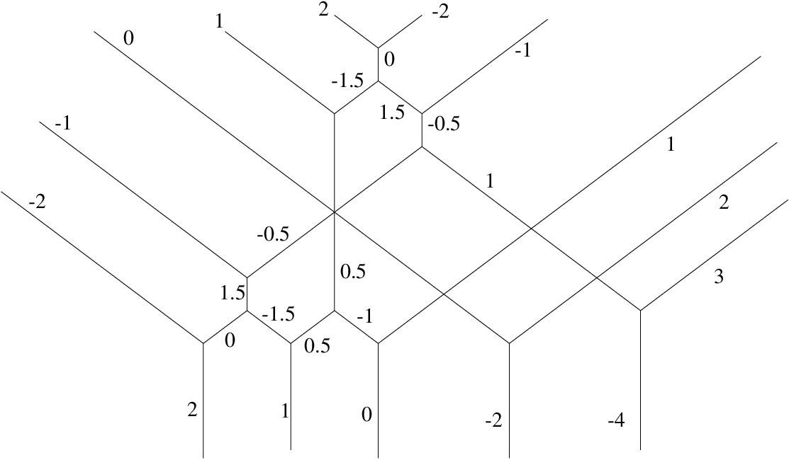
It will turn out that, in a sense, the -valent vertex is to blame for this honeycomb’s bad behavior. In this section we develop the machinery to find extremal honeycombs with better vertices (and thus better behavior) than this one.
Let be a (possibly unbounded) polyhedron in a vector space , a projection that restricts to a proper map , and a generic functional on . Define the “largest lift” map , taking to the point in with greatest pairing with . By properness, there is a point maximizing this pairing; by genericity of , this point is unique. So the map is well-defined, and in fact is continuous and piecewise-linear ([Zi, pp. 293-4]). In the case of a tortoise, its shadow on the ground at noon, and measuring the height off the ground, the largest lift of a point in the shadow is the corresponding point on the tortoise’s upper shell.
Fix a honeycomb tinkertoy . We are interested in this largest-lift map in the case of the projection , which forgets the location of the vertices and finite edges of a honeycomb, remembering only the constant coordinates on the boundary edges.
Proposition 2.
Let be the honeycomb tinkertoy. Then the map is proper.
Proof.
This is guaranteed by the correspondence with the BZ cone (in appendix 1). ∎
In fact this map is improper only if has semiinfinite edges in all six directions, but we will not need this fact in this paper.
The functional is chosen to be a generically weighted sum of the perimeters of the (possibly degenerate) hexagons in the honeycomb, the weighting having a certain “superharmonicity” property. More exactly, let assign a real number to each of the regions in the tinkertoy (vertices of ), with the properties that
- (1)
For each unbounded region on the exterior,
- (2)
for each hexagon surrounded by regions ,
- (3)
is chosen generic subject to these constraints.
(One nongeneric such can be defined on any by . But the set of is open, so we can perturb this one slightly to get a generic .)
Then we define the weighted perimeter of a -honeycomb as
Since is defined in terms of the perimeter, it’s a linear functional on .
Lemma 9.
Let be a honeycomb in which some hexagon can inflate (moving the vertices of the loop, as in lemma 2). Then inflating it increases .

Proof.
Inflating the hexagon by distance increases its perimeter by , while decreasing that of each of its neighbors by . The change in is
∎
This lemma is best understood in terms of ’s linear structure, which while transparent in the original BZ formulations, or the hive model in appendix 2, is unfortunately rather opaque in the honeycomb model. For each region in a honeycomb tinkertoy , define the inflation virtual configuration which places the vertices of around the origin in (by translating the hexagon containing ’s vertices to the hexagon in the infinite honeycomb tinkertoy around the origin), but all other vertices at the origin. Then the statement “the hexagon can inflate in , but gets stuck at a distance ” is equivalent to “ is in the cone for , but past this ray leaves the cone”. And lemma 9 above is exactly the statement (if we extend linearly to the vector space of virtual configurations of ) that .
In a particularly degenerate honeycomb it may be impossible to inflate any one hexagon; only certain combinations may be possible. This next slightly technical lemma shows that certain local changes to a honeycomb, which molt1717 17 From Webster’s: molt : to shed hair, feathers, shell, horns, or an outer layer periodically : to cast off (an outer covering) periodically; specif : to throw off (the old cuticle) the degeneracy, can be obtained by inflating several hexagons simultaneously.

Lemma 10.
The virtual configurations associated to the recipes in figure 20 for molting a degenerate vertex are in each case the sum of a set of inflation virtual configurations associated to inflating a certain collection of regions . More precisely, each molting recipe inflates equally the completely degenerate hexagons, plus the -sided regions on the sides corresponding to thick edges.
Proof.
Since these degenerate vertices involve, by definition, a number of hexagons that have collapsed (to lines and even to points), it is rather difficult to see which hexagons must be simultaneously inflated to make the vertex molt. We will use the linear structure to get around this as follows; first add times the standard configuration of the honeycomb tinkertoy . Now there is no degeneracy and we can point out which regions to inflate. Add the corresponding virtual configurations to this configuration. Then subtract times the standard configuration and see that we do get the molted configuration.
Note in particular that if we mark two adjacent regions for the same amount of inflation, their common edge doesn’t move at all. So it is simple to see whether an edge moves under simultaneous inflation, since each edge is on the boundary of exactly two regions; it moves if exactly one of them inflates, away from that one.
In each of the following pictures we show
- (1)
the vertex (edges labeled with their multiplicities)
- (2)
the standard configuration of (a small example of) the underlying tinkertoy, with certain regions labeled in gray
- (3)
the result of inflating those regions some distance
- (4)
the same result, with the standard configuration subtracted off.
Molting a Y vertex (figure 21). We determined in lemma 6 that Y vertices result from the collapse of a -type honeycomb tinkertoy. To perform the sort of molt we want here, we inflate all the regions except one corner and the opposite side.

Molting a crossing vertex (figure 22). In this case we inflate all regions except those on the left and right side. Again, we are using lemma 6 to know precisely what is hiding in the degenerate vertex, as we will again in the remaining cases.

Molting a rake vertex (figure 23). In this case we inflate all regions except those on the left, right, and top.

Molting a -valent or -valent vertex. This is more of the same, so we do not take space for the pictures (see figure 8 for the standard configurations of the tinkertoys). In both the - and -valent case, we mark all the hexagons for inflation, and in the -valent case we also mark for inflation the -sided unbounded regions on the side with external edges. ∎
Note that we make no statement here about the change in the weighted perimeter, since (except in the -valent vertex case) some of the regions we are inflating are unbounded, and lemma 9 does not pertain. In the theorem to follow we will only be inflating hexagons.
For a honeycomb tinkertoy, call a set of regular boundary conditions if no two semiinfinite edges of in the same direction are assigned the same constant coordinate. This terminology is taken from the -honeycomb case, where such boundary conditions correspond to triples of regular dominant weights (i.e. in the interior of the positive Weyl chamber).
The main result in this paper is the following.
Theorem 2.
Let be a honeycomb tinkertoy such that the map is proper, as in proposition 2. Let be a regular point in , and the largest-lift honeycomb lying over it (relative to a generic choice ). Then has only simple degeneracies, and if one elides them, the graph underlying the resulting tinkertoy is acyclic.
Proof.
Since the map is assumed proper, the concept of a “largest lift” makes sense, and we can go on to study its properties. In order, we will show
- (1)
a largest lift never has -valent vertices
- (2)
a largest lift of a regular point has no edges of multiplicity (and therefore no rakes or -valent vertices)
- (3)
a simply degenerate largest lift has no cycles.
Item is immediate from lemma 10: if has a -valent vertex, we can molt it by inflating a certain set of hexagons. But by lemma 9 that increases the weighted perimeter. So was not a largest lift, contrary to assumption.
Example 6.
In the calculation of the tensor square of ’s adjoint representation in figure 5, we found that two copies of the adjoint representation (tensor the determinant) appear. One of them has a -valent vertex and is thus not a largest lift. When that vertex “molts” as explained above (and the resulting hexagon is maximally inflated), one obtains the other honeycomb with the same boundary, which is a largest lift.
Proof of . Let be the maximum edge-multiplicity that appears in ; assume or else we’re done. Let be the subgraph of of the edges with multiplicity (and their vertices). By the assumption that is regular, this contains none of the semiinfinite edges; it is bounded. Let be a vertex on the boundary of the convex hull of ; is necessarily a rake or a -valent vertex.
Build a path in starting at , with first edge , as follows. Declare the direction clockwise of to be the “forbidden” direction, and counterclockwise to be “windward”.
Now traverse edges, coming to new vertices, going through crossings, turning at Ys (but not into the forbidden direction), stopping when you reach another rake or -valent vertex. (Conceivably one might continue through a -valent vertex, if it is lucky enough to have two edges of multiplicity , but we don’t do this.) Once you start building this path from , there are no choices, and each step carries us a positive distance in the windward direction. So the path doesn’t self-intersect, and since the graph is bounded, this algorithm must terminate. By the assumption that was the maximum edge-multiplicity, we only come into a rake or -valent along the edge labeled in lemma 10 (up to rotation and reflection).
We now attempt to simultaneously inflate all the hexagons that have completely degenerated to the vertices along , plus those that have collapsed to the edges connecting two vertices. Comparing this to the recipes in lemma 10, we see that this exactly molts all the vertices, and is thus a legal combination (adding a small multiple doesn’t carry us out of the cone ). This operation inflates some hexagons, and therefore by lemma 9 increases the weighted perimeter, violating the largest-lift assumption as before.
We give an example of this in figure 24, where an entire path molts. This illustrates how the recipes for molting at a vertex exactly fit together to give a well-defined operation on the honeycomb.

Proof of . Now that we know that our largest lift of a regular triple only has simple degeneracies, we can apply lemma 2 (or rather, its strengthened version in the corollary to theorem 1) to say that any cycle in the graph underlying the post-elision tinkertoy gives a degree of freedom. But by the assumed genericity of , our honeycomb should be at a vertex of the polytope of honeycombs lying over , and thus have no degrees of freedom. Hence there are no cycles in the post-elision tinkertoy. ∎
Honeycombs with nonsimple degeneracies can be seen in figure 5 – but only when the bottom edge has some edges lying on top of one another, or the honeycomb is not a largest lift.
6. Proof of the saturation conjecture
We prove a general honeycomb version of the saturation conjecture. Then we derive the actual representation theory saturation conjecture from its truth for -honeycomb tinkertoys.
Theorem 3.
Let be a honeycomb tinkertoy such that the projection is proper, and a generic weighting function on the regions satisfying the properties required in section 5. Then the largest-lift map is a piecewise -linear map. Consequently, any point in assigning integer constant coordinates to the boundary edges can be extended to a lattice honeycomb.
Proof.
We already know that the largest-lift map is continuous, and linear on chambers. We will show by studying regular points in that each of these linear maps has integer coefficients. Then for any point in , even nonregular, we can pick a chamber of which that point is on the boundary, and show that over that point there lies a lattice honeycomb.
If is a regular configuration in , then by theorem 2 from section 5, the largest lift honeycomb has only simple degeneracies (its vertices only look like Ys or crossing vertices, with edge-multiplicity everywhere).
By the “elision” construction in section 2, we can regard this as a nondegenerate configuration of a simpler post-elision tinkertoy, where each crossing point is removed, and the five edges (one of length zero) replaced by the two lines going through.
In this tinkertoy, each vertex is degree , touching some finite and some semiinfinite edges. Consider the subgraph of finite edges, also acyclic, and inductively pull off vertices of degree . Each such vertex is connected to two semiinfinite edges, whose constant coordinates determine the location of the vertex. In particular the constant term on the finite edge coming out is integrally determined by those on the two semiinfinite edges – it is minus their sum.
![[Uncaptioned image]](9807160v4/intdeterm.png)
So we can remove the two semiinfinite edges and the vertex, promoting the remaining edge to semiinfinite, and recurse. Eventually all the coordinates are integrally determined from those on the original semiinfinite edges. ∎
(We invite the reader to see how this argument fails on the honeycomb in figure 18.)
It may be worth noting that one can make these integral formulae very explicit. To determine the constant coordinate on a two-ended edge somewhere in the middle of this honey-forest , let be the set of semiinfinite edges such there is a path (necessarily unique) from to going through ’s right-side-up Y vertex. (Unless the post-elision tinkertoy is disconnected, the unique path from to will go either through ’s Y vertex or ’s upside-down Y vertex.) Then the constant coordinate on is the sum of the constant coordinates on the outgoing boundary edges in , minus the corresponding sum on the incoming edges.
Corollary (the saturation conjecture).
Let be a triple of dominant integral weights of such that for some , the tensor product has a -invariant vector. Then already has a -invariant vector.
Proof.
Let be the honeycomb tinkertoy. By theorem 4 from appendix 1, the fiber of the boundary-conditions map over the point contains a lattice point, and is therefore nonempty. Therefore the fiber over is also nonempty, since it just the original fiber rescaled by . By proposition 2 we can apply theorem 3, which says that this fiber contains a lattice point. Using theorem 4 again, we find that has a -invariant vector. ∎
There is an analogous saturation conjecture for the tensor product of any number of representations, which for our purposes we can state as follows. Let be a collection of dominant weights such that for some large , the tensor product has a -invariant vector. Then the same is true when is replaced by .
An earlier version of this paper had a technically unpleasant proof of the general saturation conjecture. We omit the details, because since writing this paper, Andrei Zelevinsky has shown us how to derive the general saturation result from the case already proven, via standard arguments with the Littlewood-Richardson rule [Ze]. The basic idea of the omitted proof is indicated in figure 25, which shows a honeycomb tinkertoy whose largest lifts give witnesses to saturation in the case of a seven-fold tensor product.
As long as the inputs are pulled apart sufficiently (), a configuration of this big honeycomb tinkertoy corresponds 1:1 to a ‘coherent’ set of honeycombs (they are far enough apart to necessarily not overlap when glued together into a configuration of the big honeycomb tinkertoy). That and repeated application of the isomorphism
(where runs over all irreducible representations of ) let us locate a lattice point in the analogous Berenstein-Zelevinsky polytope.
7. A saturation conjecture for other groups
One can phrase a naïve saturation conjecture for other groups : for any triple of dominant weights for , if there exists a number such that
However, this conjecture is false, with counterexamples reported in [E]. A clue is provided by the fact that it is already false for !
Of course, the case is not so different from the case, where saturation holds, and so is easily patched up; we must ask also that the representation of the torus annihilate the center of . (This is no longer a linear condition on , as it was for , exactly because ’s center is not connected.)
Conjecture.
Let be a connected complex semisimple Lie group with maximal torus , a triple of dominant weights for , and a positive number such that
Then if annihilates all elements of with semisimple centralizer,
We now explain the geometric motivation for this conjecture. Since our only goal is to make the conjecture plausible we do not waste space on full proofs of the statements made here.
The space can be thought of as the space of sections of a sheaf on the GIT quotient (as explained in the introduction, in the case of ). However, this sheaf may not necessarily be a line bundle; it can have singularities that get worse at orbifold points of the quotient, and any section is required to vanish at the singularities. The condition that annihilate the center exactly guarantees that this sheaf be a line bundle generically, so is certainly necessary for the existence of nonvanishing sections.
However, if the sheaf has singularities along which any section must vanish, it stands to reason that global sections are less likely to exist. The condition in the conjecture is exactly equivalent to asking that the sheaf be a line bundle globally, therefore to have a better chance to have sections.
To be sure, this conjecture is not nearly as satisfactory as the result for (primarily because it’s not necessary, only claimed to be sufficient), but the situation for other groups seems to be inherently less clean.
1. Appendix: The equivalence of -honeycombs with a definition of Berenstein-Zelevinsky patterns
Let be a hexagon with angles and two vertical edges. Define the torsion of to be the length of the left edge minus that of the right edge.
Proposition 3.
The torsion of and that of each rotation of agree.
Proof.
For a regular hexagon they are all zero. If one translates one edge of out from the center, the edge shrinks and its two neighboring edges grow, keeping the torsions equal. Any position of the hexagon can be achieved by composing such translations. ∎
Let be a -honeycomb. We will assign a number to each region in the honeycomb tinkertoy , other than the sectors at the three corners, using . This will turn out to be a Berenstein-Zelevinsky pattern.
- (1)
Each hexagon is assigned its torsion.
- (2)
Each semiinfinite wedge on the NE long edge of the honeycomb is assigned the length of its west edge.
- (3)
Each semiinfinite wedge on the NW long edge of the honeycomb is assigned the length of its SE edge.
- (4)
Each semiinfinite wedge on the bottom long edge of the honeycomb is assigned the length of its NE edge.
(This is set up so as to be -rotation invariant.)
For any region not on the NW long edge, the sum of the region-entries at and to the right of that point telescopes to the length of an edge, necessarily nonnegative. (Likewise for rotations.)
To determine the sum across an entire row is a little trickier. We need to relate the length of an edge to the constant coordinates on neighboring edges. Rotate the edge to align it with the finite edge in figure 26.

So the sum across an entire left-right row, with a semiinfinite wedge at the left end, is
- (1)
the sum of the lengths of the two finite edges of that wedge
- (2)
the difference of the constant coordinates of the semiinfinite edges of that wedge.
(By -rotational symmetry the same is true for sums in other directions.)
In particular, if the constant coordinates of the semiinfinite edges are interpreted as the coefficients of three dominant weights (in nonincreasing order) as in the rest of the paper, the labeling of the regions exactly matches the definition of Berenstein-Zelevinsky pattern as given in [Ze] (only one of many realizations, others to be found in the original [BZ]).
The central theorem in [BZ] gives a formula for Littlewood-Richardson coefficients as the number of BZ patterns with given boundary values. Their formulation is more suited to than calculations, and as such, they need to include a caveat that BZ patterns count the LR coefficient only if the sum of the three weights is in the root lattice of . (If the sum is not in the root lattice, the LR coefficient is obviously zero, but there are still likely to be many BZ patterns which now have no known representation-theoretic meaning.) In the -adapted formulation of this paper this caveat does not appear.
For us, the BZ theorem reads as follows:
Theorem 4.
Let be a triple of dominant weights of . Then the number of lattice -honeycombs whose semiinfinite edges, indexed clockwise from the southwest, have constant coordinates is the corresponding Littlewood-Richardson coefficient .
2. Appendix: The hive model
In this section we introduce another model of the points in the Berenstein-Zelevinsky cone, much closer to the BZ models in feel, that has the honeycomb-like property of having only “local” inequalities. It is not strictly necessary for the logic of the paper, but is very useful as an alternate model; this is particularly true if one wants to actually count tensor product multiplicities, rather than merely prove them positive. The paper [Bu] exposing our work takes this model as the fundamental one.
As was mentioned elsewhere, the primary advantage of the honeycomb model over the original BZ models is the naturality of the ‘‘overlay’’ operation; in this paper this is only used in a sort of local way, when we elide simple degeneracies. But this comes with a cost -- the linear structure on the space of honeycombs is a bit difficult to see geometrically. In addition, the degrees of freedom of the honeycomb are distinctly more obscure than in the BZ models.1818 18 In some sense, though, the strength of the honeycomb model as used in this paper that one can study the degrees of freedom left while keeping some of the inequalities pressed, which is not so easy to do in the BZ models. (And then there is the typesetting problem.)
Given a honeycomb tinkertoy, recall the dual graph defined in section 3. Define the vector space to be labelings of the vertices of by real numbers. This vector space naturally contains the lattice of integer labelings.
Recall that the embedded graph is a collection of triangles, which we refer to as the hive triangles. Of most interest to us are the rhombi formed by pairs of adjacent hive triangles. Each such rhombus has two acute vertices and two obtuse vertices. There are three possible directions a rhombus may face.

Each rhombus gives a functional on , defined as the sum at the obtuse vertices minus the sum at the acute vertices (as seen in figure 28).

This gives a rhombus inequality, asking that the rhombus functional be nonnegative. The cone in satisfying all these inequalities we denote , and we will call its elements -hives.
Proposition 4.
Let be a honeycomb tinkertoy. Then there is a -linear correspondence between configurations of , and -hives whose leftmost top entry is zero, in such a way that the constant coordinates of the boundary edges of the honeycomb are differences of boundary entries on the corresponding -hive.
Proof.
Start with a configuration of . We label the vertices in inductively, starting with a zero in the leftmost top entry, and filling in as follows: whenever we move southwest or east, we increase the value by the constant coordinate of the edge crossed; southeast, we decrease by that constant coordinate.
Our first worry is that different paths will cause us to try to fill different numbers in the same hexagon. That this doesn’t happen is a simple consequence of the sum-equals-zero property at a vertex of the honeycomb.
Second, we need to know that the result is a hive. Not surprisingly, the rhombus inequalities are equivalent to the edge lengths being nonnegative.
Lastly, since we define the hive entries by inductively adding up constant coordinates of edges, the boundary of the hive naturally ends up being the partial sums of those constant coordinates. (The sum-equals-zero property is involved in seeing this for some of the boundary edges.) ∎
Combining this with the theorem in the appendix relating -honeycombs to Littlewood-Richardson coefficients, we find that if are integral, the number of hives with boundary formed from partial sums of is a Littlewood-Richardson coefficient. (In [Bu], there is given a simple bijection between hives and a standard formulation of the Littlewood-Richardson rule.)
There is a pleasant geometric way to interpret the rhombus inequalities. Extend the hive to a piecewise linear function, affine-linear on each little hive triangle. Then the rhombus inequalities state that this function is convex. Each rhombus equality says that the function is actually linear across the boundary down the middle of the rhombus, i.e. that the regions on which the function is affine-linear are larger than just the little hive triangles.
In this way, the set of tight rhombus inequalities determines a certain decomposition of the convex region in bearing into regions (which we dub “flatspaces” due to the geometric interpretation above). This is exactly the decomposition into the regions of the degeneracy graph from section 3. We mentioned there that the degeneracy graph remembers only the “combinatorial information” about a honeycomb; we see now that it is the hive that finishes the job.
Again, we refer readers to the honeycomb/hive applet to see these hives and convex graphs in action, at
http://www.alumni.caltech.edu/˜allenk/java/honeycombs.html.
References
- [Bu] A. Buch, The saturation conjecture (after A. Knutson and T. Tao), notes from a talk at Berkeley September 1998.
- [BS] L. Billera, B. Sturmfels, Fiber polytopes, Annals of Math. 135 (1992), no. 3, 527–549.
- [BZ] A. Berenstein, A. Zelevinsky, Triple multiplicities for and the spectrum of the exterior algebra of the adjoint representation, J. Alg. Comb., 1 (1992), 7 - 22.
- [E] A.G. Elashvili, Invariant algebras, Advances in Soviet Math., 8 (1992), 57-64.
- [F] W. Fulton, Eigenvalues of sums of Hermitian matrices (after A. Klyachko), Séminaire Bourbaki. (1998).
- [FH] W. Fulton, J. Harris, Representation theory, Springer-Verlag (1991).
- [GP] O. Gleizer, A. Postnikov, Littlewood-Richardson coefficients via Yang-Baxter equation, in preparation.
- [GZ] V. Guillemin, C. Zara, Equivariant de Rham theory and graphs, math.DG/9808135.
- [H] A. Horn, Eigenvalues of sums of Hermitian matrices, Pacific J. Math., 12 (1962), 225-241.
- [Hon2] A. Knutson, T. Tao, C. Woodward, The honeycomb model of tensor products II: Facets of the L-R cone, in preparation.
- [KSZ] M. Kapranov, B. Sturmfels, A. Zelevinsky, Quotients of toric varieties. Math. Annalen. 290 (1991), no. 4, 643–655.
- [Kl] A.A. Klyachko, Stable vector bundles and Hermitian operators, IGM, University of Marne-la-Vallee preprint (1994).
- [KMP] S. Kumar, Proof of the Parthasarathy-Ranga Rao-Varadarajan conjecture. Invent. math. 93 (1988), no. 1, 117–130. O. Mathieu, Construction d’un groupe de Kac-Moody et applications. Compositio Math. 69 (1989), no. 1, 37–60. P. Polo, Variétés de Schubert et filtrations excellentes. Astérisque. 10-11 (1989) 281-311.
- [Ku] G. Kuperberg, Spiders for rank two Lie algebras, math.QA/9712143, Comm. Math. Phys., 180(1):109-151, 1996
- [MFK, chapter 8] D. Mumford, J. Fogarty, F. Kirwan, Geometric invariant theory. Third edition. Ergebnisse der Mathematik und ihrer Grenzgebiete, Springer-Verlag, 1994.
- [Ze] A. Zelevinsky, Littlewood-Richardson semigroups, math.CO/9704228.
- [Zi, pp. 293-4] G. Ziegler, Lectures on polytopes, Graduate Texts in Mathematics, 152. Springer-Verlag, 1995.