Tessellations of moduli spaces and the mosaic operad
Abstract.
We construct a new (cyclic) operad of mosaics defined by polygons with marked diagonals. Its underlying (aspherical) spaces are the sets which are naturally tiled by Stasheff associahedra. We describe them as iterated blow-ups and show that their fundamental groups form an operad with similarities to the operad of braid groups.
Acknowledgments.
This paper is a version of my doctorate thesis under Jack Morava, to whom I am indebted for providing much guidance and encouragement. Work of Davis, Januszkiewicz, and Scott has motivated this project from the beginning and I would like to thank them for many useful insights and discussions. A letter from Professor Hirzebruch also provided inspiration at an early stage. I am especially grateful to Jim Stasheff for bringing up numerous questions and for his continuing enthusiasm about this work.
1. The Operads
1.1.
The notion of an operad was created for the study of iterated loop spaces [13]. Since then, operads have been used as universal objects representing a wide range of algebraic concepts. We give a brief definition and provide classic examples to highlight the issues to be discussed.
Definition 1.1.1.
An operad is a collection of objects in a monoidal category endowed with certain extra structures:
1. carries an action of the symmetric group .
This paper will be concerned mostly with operads in the context of topological spaces, where the objects will be equivalence classes of geometric objects.
Example 1.1.2.
These objects can be pictured as trees (Figure 1a). A tree is composed of corollas11 1 A corolla is a collection of edges meeting at a common vertex. with one external edge marked as a root and the remaining external edges as leaves. Given trees and , basic compositions are defined as , obtained by grafting the root of to the leaf of . This grafted piece of the tree is called a branch.

Example 1.1.3.
There is a dual picture in which bubbles replace corollas, marked points replace leaves, and the root is denoted as a point labeled (Figure 1b). Using the above notation, the composition is defined by fusing the of the bubble with the marked point of . The branches of the tree are now identified with double points, the places where bubbles intersect.
1.2.
Taking yet another dual, we can define an operad structure on a collection of polygons (modulo an appropriate equivalence relation) as shown in Figure 1c. Each bubble corresponds to a polygon, where the number of marked and double points become the number of sides; the fusing of points is associated with the gluing of faces. The nicest feature of polygons is that, unlike corollas and bubbles, the iterated composition of polygons yields a polygon with marked diagonals (Figure 2).

Unlike the rooted trees, this mosaic operad is cyclic in the sense of Getzler and Kapranov [7, §2]. The most basic case (Figure 3) shows how two polygons, with sides labeled and respectively, compose to form a new polygon. The details of this operad are made precise in §2.2.

1.3.
In the work of Boardman and Vogt [1, §2.6], an operad is presented using dimensional cubes . An element of this little cubes operad is the space of an ordered collection of cubes linearly embedded by , with disjoint interiors and axes parallel to . The ’s are uniquely determined by the -tuple of points in , corresponding to the images of the lower and upper vertices of . An element acts on by permuting the labeling of each cube:
The composition operation (1.1) is defined by taking spaces (each having embedded cubes) and embedding them as an ordered collection into . Figure 4 shows an example for the two dimensional case when .

Boardman showed that the space of distinct cubes in is homotopically equivalent to , the configuration space on distinct labeled points in .22 2 The equivariant version of this theorem is proved by May in [13, §4]. When , is homeomorphic to , where is the thick diagonal . Since the action of on is free, taking the quotient yields another space . It is well-known that both these spaces are aspherical, having all higher homotopy groups vanish [4]. The following short exact sequence of fundamental groups results:
But of is simply , the pure braid group. Similarly, of quotiented by all permutations of labelings is the braid group . Therefore, the short exact sequence above takes on the more familiar form:
We will return to these ideas in §6.
2. The Moduli Space
2.1.
The moduli space of Riemann spheres with punctures,
has been studied extensively [10]. It has a Deligne-Mumford-Knudsen compactification , a smooth variety of complex dimension . In fact, this variety is defined over the integers; we will look at the real points of this space. These are the set of fixed points of under complex conjugation.
Definition 2.1.1.
The moduli space of configurations of smooth points on punctured stable real algebraic curves of genus zero is a compactification of the quotient where is the thick diagonal.
Remark.
This is an action of a non-compact group on a non-compact space. Geometric invariant theory gives a natural compactification for this quotient, defined combinatorially in terms of bubble trees or algebraically as a moduli space of real algebraic curves of genus zero with points, which are stable in the sense that they have only finitely many automorphisms.
A point of can be visualized as a bubble (that is, ) with distinct labeled points. For a particular labeling, the configuration space of such points gives us a fundamental domain of . There are possible labelings. However, since there exists a copy of the dihedral group in , and since is defined as a quotient by , two labeled bubbles are identified by an action of . Therefore, there are copies of the fundamental domain that make up . Since we remove the thick diagonal, these domains are open cells.
In , however, these marked points are allowed to ‘collide’ in the following sense: As two adjacent points and of the bubble come closer together and try to collide, the result is a new bubble fused to the old at the point of collision (a double point), where the marked points and are now on the new bubble (Figure 5). Note that each bubble must have at least three marked or double points in order to be stable.

The mosaic operad encapsulates all the information of the bubbles, enabling one to look at the situation above from the vantage point of polygons. Having marked points on a circle now corresponds to an -gon; when two adjacent sides and of the polygon try to collide, a diagonal of the polygon is formed such that and lie on one side of the diagonal (Figure 6).

What is quite striking about is that its homotopy properties are completely encapsulated in the fundamental group.
Theorem 2.1.2.
[5, §5.1] is aspherical.
We will return to the structure of the fundamental group in §6.
2.2.
We now turn to defining the mosaic operad and relating its properties with the structure of . Let be the unit circle bounding , the disk endowed with the Poincaré metric; this orients the circle. The geodesics in correspond to open diameters of together with open circular arcs orthogonal to . The group of isometries on is [15, §4].
A configuration of distinct points on defines an ideal polygon in , with all vertices on the circle and geodesic sides. Let be the space of such configurations, modulo , and let be the space of such ideal polygons marked with non-intersecting geodesics between non-adjacent vertices. We want to think of the elements of as limits of configurations in in which sets of points have coalesced (see discussion above). Specifying diagonals defines a decomposition of an -gon into smaller polygons, and we can topologize as a union of -fold products of ’s corresponding to this decomposition. For example, to the one dimensional space we attach zero dimensional spaces of the form . The combinatorics of these identifications can be quite complicated, but Stasheff’s associahedra were invented to solve just such problems, as we will see in §2.3 below.
Henceforth, we will visualize elements of as -gons with non-intersecting diagonals, and we write for the space of -gons with any number of such diagonals. Elements of inherit a natural cyclic order on their sides, and we write for the space of -gons with labeled sides.
Proposition 2.2.1.
There exists a bijection between the points of and the elements of .
Remark.
Given an element in , we can associate to it a dual tree. Its vertices are the barycenters of polygons, defined using the Riemann mapping theorem, and the branches are geodesics between barycenters. The leaves are geodesics that extend to points on midway between two adjacent marked points on . It then follows that is a space of hyperbolic planar trees. This perspective naturally gives a Riemann metric to .
Definition 2.2.2.
Given and (where ), there are composition maps
where . The object is obtained by gluing side of along side of . The symmetric group acts on by permuting the labeling of the sides. These operations define the mosaic operad .
Remark.
The one dimensional case of the little cubes operad is , the little intervals operad. An element is an ordered collection of embeddings of the interval , with disjoint interiors. The notion of trees and bubbles, shown in Figure 1, is encapsulated in this intervals operad. Furthermore, after embedding in and identifying with , the mosaic operad becomes a compactification of .
2.3.
We now define the fundamental domain of as a concrete geometric object and present its connections with the mosaic operad.
Definition 2.3.1.
Let be the space of distinct points on the interval such that . Identifying with carries the set of points onto . Therefore, there exists a natural inclusion of in . Define the associahedron as the closure of the space in .
Proposition 2.3.2.
An interior point of corresponds to an element of , and an interior point of a codim face corresponds to an element of .
Proof.
Since , one can fix three of the distinct points on to be and . Thus, the associahedron can be identified with the cell tiling and the proposition follows from the construction of . ∎
The relation between the -gon and is further highlighted by a work of Lee [12], where he constructs a polytope that is dual to , with one vertex for each diagonal and one facet for each triangulation of an -gon. He then proves the symmetry group of to be the dihedral group . Restated, it becomes
Proposition 2.3.3.
[12, §5] acts as a group of isometries on .
Historical Note.
Stasheff classically defined the associahedron for use in homotopy theory [16, §6] as a CW-ball with codim faces corresponding to using sets of parentheses meaningfully on letters.33 3 From the definition above, the letters can be viewed as the points . It is easy to describe the associahedra in low dimensions: is a point, a line, and a pentagon. The two descriptions of the associahedron, using polygons and parentheses, are compatible: Figure 7 illustrates as an example. The associahedra have continued to appear in a vast number of mathematical fields, gradually acquiring more and more structure, cf. [19].

2.4.
The polygon relation to the associahedron enables the use of the mosaic operad structure on .
Proposition 2.4.1.
[16, §2] Each face of is a product of lower dimensional associahedra.
In general, the codim face of the associahedron will decompose as
where and . This parallels the mosaic operad structure
where , and the gluing of sides is arbitrary. Therefore, the product in Proposition 2.4.1 is indexed by the internal vertices of the tree corresponding to the face of the associahedron.
Example 2.4.2.
We look at the codim one faces of . The three dimensional corresponds to a 6-gon, which has two distinct ways of adding a diagonal. One way, in Figure 8a, will allow the 6-gon to decompose into a product of two 4-gons (’s). Since is a line, this codim one face yields a square. The other way, in Figure 8b, decomposes the 6-gon into a 3-gon () and a 5-gon (). Taking the product of a point and a pentagon results in a pentagon.

Example 2.4.3.
We look at the codim one faces of . Similarly, Figure 9 shows the decomposition of the codim one faces of , a pentagonal prism and .

3. The Tessellation
3.1.
We extend the combinatorial structure of the associahedra to . Propositions 2.2.1 and 2.3.2 show the correspondence between the associahedra in and . We investigate how these copies of glue to form .
Definition 3.1.1.
Let and be a diagonal of . A twist along , denoted by , is the element of obtained by ‘breaking’ along into two parts, ‘twisting’ one of the pieces, and ‘gluing’ them back (Figure 10).

The twisting operation is well-defined since the diagonals of an element in do not intersect. Furthermore, it does not matter which piece of the polygon is twisted since the two results are identified by an action of . It immediately follows that the identity element.
Proposition 3.1.2.
Two elements, , representing codim faces of associahedra, are identified in if there exist diagonals of such that
Proof.
As two adjacent points and on collide, the result is a new bubble fused to the old at a point of collision , where and are on the new bubble. The location of the three points on the new bubble is irrelevant since . In terms of polygons, this means does not affect the cell, where is the diagonal representing the double point . In general, it follows that the labels of triangles can be permuted without affecting the cell. Let be an -gon with diagonal partitioning into a square and an -gon. Figure 11 shows that since the square decomposes into triangles, the cell corresponding to is invariant under the action of . Since any partition of by a diagonal can be decomposed into triangles, it follows by induction that does not affect the cell. ∎

Theorem 3.1.3.
There exists a surjection
which is a bijection on the interior of the cells. In particular, copies of tessellate .
3.2.
In Figure 12, a piece of represented by labeled polygons with diagonals is shown. Note how two codim one pieces (lines) glue together and four codim two pieces (points) glue together. Understanding this gluing now becomes a combinatorial problem related to .

Notation.
Let be the number of codim cells in a CW-complex . For a fixed codim cell in , and for , let be the number of codim cells in whose boundary contains the codim cell. Note the number is well-defined by Theorem 3.1.3.
Lemma 3.2.1.
Proof.
This is obtained by just counting the number of -gons with non-intersecting diagonals, done by A. Cayley in 1891 [3]. ∎
Lemma 3.2.2.
Proof.
The boundary components of a cell corresponding to an element in are obtained by adding non-intersecting diagonals. To look at the coboundary cells, diagonals need to be removed. For each diagonal removed, two cells result (coming from the twist operation); removing diagonals gives cells. We then look at all possible ways of removing out of diagonals. ∎
Theorem 3.2.3.
| (3.1) |
Proof.
Remark.
Professor F. Hirzebruch has kindly informed us that he has shown, using techniques of Kontsevich and Manin [11], that the signature of is given by (3.1). He remarks that the equivalence of this signature with the Euler number of the space of real points is an elementary consequence of the Atiyah-Singer -signature theorem.
4. The Hyperplanes
4.1.
Another approach to is from a top-down perspective using hyperplane arrangements as formulated by Kapranov [8, §4.3] and described by Davis, Januszkiewicz, and Scott [5, §0.1].
Definition 4.1.1.
Let be the hyperplane defined by . For , let be the hyperplane defined by . The braid arrangement is the collection of subspaces of generated by all possible intersections of the .
If denotes the collection of subspaces , then cuts into simplicial cones. Let be the sphere in and let be the projective sphere in (that is, ). Let to be the intersection of with ; the arrangement cuts into open simplices.
Definition 4.1.2.
Let be a codim irreducible cell of if hyperplanes of intersect there.44 4 The use of the word irreducible comes from [5] in reference to Coxeter groups.
Example 4.1.3.
We look at the case when . Figure 13 shows the ‘scars’ on the manifolds made by . On , there are four places where three hyperplanes intersect, corresponding to the four codim two irreducible points.

Definition 4.1.4.
Replace with , the sphere bundle associated to the normal bundle of . This process yields a manifold with boundary. Then projectify into , the projective sphere bundle. This defines a manifold without boundary, called the blow-up of along .
Remark.
Replacing with for any dimension creates a new manifold with boundary. However, blowing up along defines a new manifold for all dimensions except codim one. That is, for codim one, projectifying into annuls the process of replacing with .
Proposition 4.1.5.
[8, §4.3] The iterated blow-up of along the cells in increasing order of dimension yields . It is inessential to specify the order in which cells of the same dimension are blown up.
Therefore, the compactification of is obtained by replacing the set with . The closure of in is obtained by replacing the set with {}; this procedure truncates each simplex of into the associahedron . We explore this method of truncation in §5.4.
Example 4.1.6.
The blow-up of yielding is shown in Figure 14. The arrangement on yields six lines forming twelve -simplices; the irreducible components of codim two turn out to be the points of triple intersection. Blowing up along these components, we get as a hexagon for and as a triangle for . The associahedron is a pentagon, and the space becomes tessellated by twelve such cells (shaded), an “evil twin” of the dodecahedron. appears as the connected sum of five real projective planes.

4.2.
Another way of looking at the moduli space comes from observing the inclusion . Since is defined as distinct points on quotiented by , one can fix three of these points to be and . From this perspective we see that is a point. When , the cross-ratio is a homeomorphism from to , the result of identifying three of the four points with and . In general, becomes a manifold blown up from an dimensional torus, coming from the -fold products of . Therefore, the moduli space before compactification can be defined as
where at least 3 points collide}. Compactification is accomplished by blowing up along .
Example 4.2.1.
An illustration of from this perspective appears in Figure 15. From the five marked points on , three are fixed leaving two dimensions to vary, say and . The set is made up of seven lines and , giving a space tessellated by six squares and six triangles. Furthermore, becomes the set of three points ; blowing up along these points yields the space tessellated by twelve pentagons. This shows as the connected sum of a torus with three real projective planes.

Example 4.2.2.
In Figure 16, a rough sketch of is shown as the blow-up of a three torus. The set associated to has ten lines {} and {}, and three points {}. The lines correspond to the hexagonal prisms, nine cutting through the faces, and the tenth (hidden) running through the torus from the bottom left to the top right corner. The three points correspond to places where four of the prisms intersect.
The shaded region has three squares and six pentagons as its codim one faces. In fact, all the top dimensional cells that form turn out to have this property; these cells are the associahedra (see Figure 9b).

4.3.
We now introduce a construction which clarifies the structure of .
Definition 4.3.1.
[9, §4] A double cover of , denoted by , is obtained by fixing the marked point on to be and assigning it an orientation.55 5 Kapranov uses the notation to represent this double cover.
Example 4.3.2.
Figure 17 shows the polygon labelings of and , being tiled by six and three copies of respectively. In this figure, the label has been set to . Note that the map is the antipodal quotient.

The double cover can be constructed using blow-ups similar to the method described above; instead of blowing up the projective sphere , we blow-up the sphere . Except for the anomalous case of , the double cover is a non-orientable manifold. Note also that the covering map is the antipodal quotient, coming from the map . Being a double cover, will be tiled by copies of .66 6 These copies of are in bijection with the vertices of the permutohedron [9]. It is natural to ask how these copies glue to form .
Definition 4.3.3.
A marked twist of an -gon along its diagonal , denoted by , is the polygon obtained by breaking along into two parts, reflecting the piece that does not contain the side labeled , and gluing them back together.
The two polygons at the right of Figure 10 turn out to be different elements in , whereas they are identified in by an action of . The following is an immediate consequence of the above definitions and Theorem 3.1.3.
Corollary 4.3.4.
There exists a surjection
which is a bijection on the interior of the cells.
Remark.
The spaces on the left define the classical operad [7, §2.9].
Theorem 4.3.5.
The following diagram is commutative:
where the vertical maps are antipodal identifications and the horizontal maps are a quotient by .
Proof.
Look at by associating to each a particular labeling of an -gon. We obtain by gluing the associahedra along codim one faces using (keeping the side labeled fixed). It follows that two associahedra will never glue if their corresponding -gons have labeled on different sides of the polygon. This partitions into , with each element of corresponding to labeled on a particular side of the -gon. Furthermore, Corollary 4.3.4 tells us that each set of the copies of glue to form . Therefore, ∎
5. The Blow-Ups
5.1.
The spaces and differ only by blow-ups, making the study of their structures crucial. Looking at the arrangement on , there turn out to be irreducible points in general position. In other words, these points can be thought of as vertices of an simplex with an additional point at the center. Between every two points of , there exists a line, resulting in such irreducible lines. In general, irreducible points of span a dimensional irreducible cell; restating this, we get
Proposition 5.1.1.
The number of irreducible components in equals
| (5.1) |
The construction of the braid arrangement shows that around a point of , the structure of resembles the barycentric subdivision of an simplex. We look at some concrete examples to demonstrate this.
Example 5.1.2.
In the case of , Figure 14a shows the cells in general position; there are four points, three belonging to vertices of a -simplex, and one in the center of this simplex. Between every two of these points, there exists a ; we see six such lines. Since these lines are of codim one, they need not be blown up. Figure 14b shows the structure of a blown up point in . Notice that is a hexagon and is a triangle. It is no coincidence that these correspond exactly to and (see Figure 17).
Example 5.1.3.
For the three dimensional , the cells and the cells need to be blown up, in that order. Choose a codim three cell ; a neighborhood around will resemble the barycentric subdivision of a -simplex. Figure 18 shows four tetrahedra, each being made up of six tetrahedra (some shaded), pulled apart in space such that when glued together the result will constitute the aforementioned subdivision. The barycenter is the point .

The left-most piece of Figure 19 shows one of the tetrahedra from Figure 18. The map takes the barycenter to whereas the map takes each going through the barycenter to . When looking down at the resulting ‘blown up’ tetrahedron piece, there are six pentagons (shaded) with a hexagon hollowed out in the center. Taking to turns these hexagons into triangles.

Putting the four ‘blown up’ tetrahedra pieces together, the faces of make up a two dimensional sphere tiled by 24 pentagons, with 8 hexagons (with antipodal maps) cut out. This turns out to be ; projectifying to yields as shown in Figure 20.

This pattern seems to indicate that for , blowing up along the point will yield . But what happens in general, when a codim cell is blown up? A glimpse of the answer was seen above with regard to the hexagons and triangles showing up in .
5.2.
To better understand , we analyze the structure of before blow-ups and after blow-ups. This is done through the eyes of mosaics, looking at the faces of associahedra surrounding each blown up component of . The following is a corollary of Proposition 5.1.1.
Corollary 5.2.1.
Each irreducible cell corresponds to a choice of elements from the set .
Choose an arbitrary and assign it such a choice, say , where . We can think of this as an -gon having a diagonal partitioning it such that labeled sides lie on one side and labeled sides lie on the other. Using the mosaic operad structure, decomposes the -gon into , where and , with the new sides of coming from . Note that corresponds to the product of associahedra .
There are different ways in which can be arranged to label . However, since twisting is allowed along , we get different labelings of , each corresponding to a . But observe that this is exactly how one gets , where the associahedra glue as defined in §3.1. Therefore, a fixed labeling of gives ; all possible labelings result in
Theorem 5.2.2.
In , each irreducible cell in becomes
| (5.2) |
Example 5.2.3.
Example 5.2.4.
Although blowing up along codim one components does not affect the resulting manifold, we observe their presence in . From (5.1), we get six such cells which become after blow-ups. The ’s are seen in Figure 14 as the six lines cutting through . Note that every line is broken into six parts, each part being a .
Example 5.2.5.
The space , illustrated in Figure 16, moves a dimension higher.77 7 Although this figure is not constructed from the braid arrangement, it is homeomorphic to the structure described by the braid arrangement. There are ten cells, each becoming . These are the hexagonal prisms that cut through the three torus as described in Example 4.2.2.
5.3.
The question arises as to why appears in . The answer lies in the braid arrangement of hyperplanes. Taking as an example, blowing up along each point in uses the following procedure: A small spherical neighborhood is drawn around and the inside of the sphere is removed, resulting in . Observe that this sphere (which we denote as ) is engraved with great arcs coming from . Projectifying, becomes , and becomes the projective sphere . Amazingly, the engraved arcs on are , and can be thought of as . Furthermore, blowing up along the lines of corresponds to blowing up along the points of in . As before, this new etching on translates into an even lower dimensional braid arrangement, .
It is not hard to see how this generalizes in the natural way: For , the iterated blow-ups along the cells up to in turn create braid arrangements within braid arrangements. Therefore, is seen in .
5.4.
So far we have been looking at the structure of the irreducible cells before and after the blow-ups. We now study how the simplex (tiling ) is truncated by blow-ups to form (tiling ).88 8 For a detailed construction of this truncation from another perspective, see Appendix B of [17]. Given a regular -gon with one side marked , define to be the set of such polygons with one diagonal.
Definition 5.4.1.
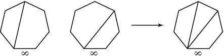
For , create a new polygon (with two diagonals) by superimposing the images of and on each other (Figure 21). and are said to satisfy the condition if has non-intersecting diagonals.
Remark.
It follows from §2.3 that elements of correspond bijectively to the codim one faces of . They are adjacent faces in if and only if they satisfy the condition. Furthermore, the codim two cell of intersection in corresponds to the superimposed polygon.
The diagonal of each element partitions the -gon into two parts, with one part not having the label; call this the free part of . Define the set to be elements of having sides on their free parts. It is elementary to show that the order of is (for ). In particular, the order of is , the number of sides (codim one faces) of an simplex. Arbitrarily label each face of the simplex with an element of .
Remark.
For some adjacent faces of the simplex, the condition is not satisfied. This is an obstruction of the simplex in becoming . As we continue to truncate the cell, more faces will begin to satisfy the condition. We note that once a particular labeling is chosen, the labels of all the new faces coming from truncations (blow-ups) will be forced.
When the zero dimensional cells are blown up, two vertices of the simplex are truncated. The labeling of the two new faces corresponds to the two elements of . We choose the vertices and the labels such that the condition is satisfied with respect to the new faces and their adjacent faces. Figure 22 shows the case for the -simplex and (compare with Figure 14).

The blow-up of one dimensional cells results in the truncation of three lines. As before, the labels of the three new faces correspond to the three elements of , choosing edges and the labels such that the condition is satisfied with respect to the new faces and their adjacent faces. Figure 23 shows the case for the -simplex and (compare with Figures 18 and 19).

As we iterate the blow-ups in Proposition 4.1.5, we jointly truncate the simplex using the above process. The blow-ups of the codim irreducible cells add new faces to the polytope, each labeled with an element from . Note that Corollary 5.2.1 is in agreement with this procedure: Each irreducible cell corresponds to a choice of labels which are used on the elements of . In the end, we are left with faces of the truncated polytope, matching the number of codim one faces of .
6. The Fundamental Group
6.1.
Coming full circle, we look at connections between the little cubes and the mosaic operads. We would like to thank M. Davis, T. Januszkiewicz, and R. Scott for communicating some of their results in preliminary form [6]. Their work is set up in the full generality of Coxeter groups and reflection hyperplane arrangements, but we explain how it fits into the notation of polygons and diagonals.
Definition 6.1.1.
Let , with diagonals respectively, satisfy the condition. Let be the element in after removing diagonal from . We then say that and are conjugate in . Figure 24 shows such a case.

Definition 6.1.2.
Let be a group generated by elements , in bijection with the elements of , with the following relations:
| if and are conjugate in | |
| if and satisfy the condition and |
The machinery above is introduced in order to understand . Fix an ordering of and use it to label the sides of each element in . We define a map as follows: Let be the product of transpositions corresponding to the permuted labels of under . Figure 25 gives a few examples.

It is not too difficult to show that the relations of carry over to . Furthermore, the transpositions form a set of generators for , showing to be surjective.99 9 To see this, simply consider the elements of . This leads to the following
Theorem 6.1.3.
[6, §4]
6.2.
The pair-of-pants product (Figure 26) takes and marked points on to marked points. The operad structure on the spaces , its simplest case corresponding to the pair-of-pants product, defines composition maps analogous to the juxtaposition map of braids.

We can thus construct a monoidal category which has finite ordered sets as its objects and the group as the automorphisms of a set of cardinality , all other morphism sets being empty. Note the following similarity between the braid group obtained from the little cubes operad and the ‘quasibraids’ obtained from the mosaic operad:
There are deeper analogies between these structures which have yet to be studied.
References
- [1] J. M. Boardman, R. M. Vogt, Homotopy invariant algebraic structures on topological spaces, Lecture Notes in Math. 347 (1973).
- [2] H. R. Brahana, A. M. Coble, Maps of twelve countries with five sides with a group of order 120 containing an Ikosahedral subgroup, Amer. J. Math. 48 (1926) 1-20.
- [3] A. Cayley, On the partitions of a polygon, Proc. Lond. Math. Soc. 22 (1890-91) 237-262.
- [4] R. Charney, M. Davis, Finite ’s for Artin Groups, Prospects in Topology (ed. F. Quinn), Annals of Math. Studies 138 (1995) 110-124.
- [5] M. Davis, T. Januszkiewicz, R. Scott, Nonpositive curvature of blowups, Selecta Math. 4 (1998) 491 - 547.
- [6] M. Davis, T. Januszkiewicz, R. Scott, The fundamental group of minimal blow-ups, in preparation.
- [7] E. Getzler, M. M. Kapranov, Cyclic operads and cyclic homology, Geometry, Topology, and Physics for Raoul Bott, ed. S. T. Yau, International Press (1994).
- [8] M. M. Kapranov, Chow quotients of Grassmannians I, Adv. in Sov. Math. 16 (1993) 29-110.
- [9] M. M. Kapranov, The permutoassociahedron, Mac Lane’s coherence theorem, and asymptotic zones for the equation, J. Pure Appl. Alg. 85 (1993) 119-142.
- [10] S. Keel, Intersection theory of moduli spaces of stable -pointed curves, Trans. Amer. Math. Soc. 330 (1992) 545-574.
- [11] M. Kontsevich, Y. Manin, Gromov-Witten classes, quantum cohomology, and enumerative geometry, Comm. Math. Phys. 164 (1994) 525-562.
- [12] C. Lee, The associahedron and triangulations of the -gon, European J. Combin. 10 (1989) 551-560.
- [13] J. P. May, The geometry of iterated loop spaces, Lecture Notes in Math. 271 (1972).
- [14] J. P. May, Definitions: operads, algebras and modules, Contemp. Math. 202 (1997) 1-7.
- [15] J. G. Ratcliffe, Foundations of hyperbolic manifolds, Grad. Text. in Math. 149, Springer-Verlag (1994).
- [16] J. D. Stasheff, Homotopy associativity of -spaces I, Trans. Amer. Math. Soc. 108 (1963) 275-292.
- [17] J. D. Stasheff (Appendix B coauthored with S. Shnider), From operads to ‘physically’ inspired theories, Contemp. Math. 202 (1997) 53-81.
- [18] M. Yoshida, Hypergeometric functions, my love, Vieweg (1997).
- [19] G. M. Ziegler, Lectures on polytopes, Grad. Text. in Math. 152, Springer-Verlag (1995).