Genus two Heegaard splittings
of orientable
three–manifolds
Abstract
It was shown by Bonahon–Otal and Hodgson–Rubinstein that any two genus–one Heegaard splittings of the same –manifold (typically a lens space) are isotopic. On the other hand, it was shown by Boileau, Collins and Zieschang that certain Seifert manifolds have distinct genus–two Heegaard splittings. In an earlier paper, we presented a technique for comparing Heegaard splittings of the same manifold and, using this technique, derived the uniqueness theorem for lens space splittings as a simple corollary. Here we use a similar technique to examine, in general, ways in which two non-isotopic genus–two Heegard splittings of the same -manifold compare, with a particular focus on how the corresponding hyperelliptic involutions are related.
keywords
Heegaard splitting, Seifert manifold, hyperelliptic involutionMartin Scharlemann
2 \volumeyear1999 \volumenameProceedings of the Kirbyfest \pagenumbers489553 \papernumber24 \published22 November 1999 \nocolon
Genus two Heegaard splittings of orientable three-manifolds
Mathematics Department, University of California
Santa Barbara, CA 93106, USA
\asciiaddressDepartment of Mathematics, University of Melbourne
Parkville, Vic 3052, Australia
Mathematics Department, University of California
Santa Barbara, CA 93106, USA
It was shown by Bonahon-Otal and Hodgson-Rubinstein that any two genus-one Heegaard splittings of the same 3-manifold (typically a lens space) are isotopic. On the other hand, it was shown by Boileau, Collins and Zieschang that certain Seifert manifolds have distinct genus-two Heegaard splittings. In an earlier paper, we presented a technique for comparing Heegaard splittings of the same manifold and, using this technique, derived the uniqueness theorem for lens space splittings as a simple corollary. Here we use a similar technique to examine, in general, ways in which two non-isotopic genus-two Heegard splittings of the same 3-manifold compare, with a particular focus on how the corresponding hyperelliptic involutions are related.
57N10 \secondaryclass57M50 \makeshorttitle
1 Introduction
It is shown in [5], [9] that any two genus one Heegaard splittings of the same manifold (typically a lens space) are isotopic. On the other hand, it is shown in [1], [14] that certain Seifert manifolds have distinct genus two Heegaard splittings (see also Section 3 below). In [16] we present a technique for comparing Heegaard splittings of the same manifold and derive the uniqueness theorem for lens space splittings as a simple corollary. The intent of this paper is to use the technique of [16] to examine, in general, how two genus two Heegard splittings of the same –manifold compare.
One potential way of creating genus two Heegaard split –manifolds is to “stabilize” a splitting of lower genus (see [17, Section 3.1]). But since, up to isotopy, stabilization is unique and since genus one Heegaard splittings are known to be unique, this process cannot produce non-isotopic splittings. So we may as well restrict to genus two splittings that are not stabilized. A second way of creating a –manifold equipped with a genus two Heegaard splitting is to take the connected sum of two –manifolds, each with a genus one splitting. But (again since genus one splittings are unique) any two Heegaard splittings of the same manifold that are constructed in this way can be made to coincide outside a collar of the summing sphere. Within that collar there is one possible difference, a “spin” corresponding to the non-trivial element of , where parameterizes unoriented planes in –space and the spin reverses the two sides of the plane. Put more simply, the two splittings differ only in the choice of which side of the torus in one summand is identified with a given side of the splitting torus in the other summand. The first examples of this type are given in [13], [19].
These easier cases having been considered, interest will now focus on genus two splittings that are “irreducible” (see [17, Section 3.2]). It is a consequence of [7] that a genus two splitting which is irreducible is also “strongly irreducible” (see [17, Section 3.3], or the proof of Lemma 8.2 below). That is, if is a Heegaard splitting, then any pair of essential disks, one in and one in , have boundaries that intersect in at least two points.
The result of our program is a listing, in Sections 3 and 4, of all ways in which two strongly irreducible genus two Heegaard splittings of the same closed orientable –manifold compare. The proof that this is an exhaustive listing is the subject of the rest of the paper. What we do not know is when two Heegaard splittings constructed in the ways described are authentically different. That is, we do not have the sort of algebraic invariants which would allow us to assert that there is no global isotopy of that carries one splitting into another. For the case of Seifert manifolds (eg [6]) such algebraic invariants can be (non-trivially) derived from the very explicit form of the fundamental group.
Any –manifold with a genus two Heegaard splitting admits an orientation preserving involution whose quotient space is and whose branching locus is a –bridge knot (cf [2]). The examples constructed in Section 4 are sufficiently explicit that we can derive from them global theorems. Here are a few: If is an atoroidal closed orientable –manifold then the involutions coming from distinct Heegaard splittings necessarily commute. More generally, the commutator of two different involutions can be obtained by some composition of Dehn twists around essential tori in . Finally, two genus two splittings become equivalent after a single stabilization.
The results we obtain easily generalize to compact orientable –manifolds with boundary, essentially by substituting boundary tori any place in which Dehn surgery circles appear.
We expect the methods and results here may be helpful in understanding –bridge knots (which appear as branch sets, as described above) and in understanding the mapping class groups of genus two –manifolds.
The authors gratefully acknowledge the support of, respectively, the Australian Research Council and both MSRI and the National Science Foundation.
2 Cabling handlebodies
Imbed the solid torus in as . Define a natural orientation-preserving involution by . Notice that the fixed points of are precisely the two arcs and the quotient space is . On the torus the fixed points of are the four points .
For any pair of integers we can define the torus link to be . The torus link is a meridian and the torus link is a longitude of the solid torus. A torus knot is a torus link of one component which is not a meridian or longitude. In other words, a torus knot is a torus link in which and are relatively prime, and neither is zero. Up to orientation preserving homeomorphism of (given by Dehn twists) we can also assume, for a torus knot, that .
Remark\quaLet be a torus knot, an arc that spans the annulus and be a radius of the disk . Then the complement of a neighborhood of in is isotopic to a neighborhood of in . This fact is useful later in understanding how cabling is affected by stabilization.
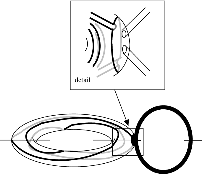
Clearly preserves any torus link . If is a torus knot, so and can’t both be even, the involution has precisely two fixed points: and either , if and are both odd; or if is even; or if is even. This has the following consequence. Let be an equivariant neighborhood of the torus knot in . Then is topologically a solid torus, and the fixed points of are two arcs. That is, is topologically conjugate to . (See Figure 1.)

The involution can be used to build an involution of a genus two handlebody as follows. Create by attaching together two copies of along an equivariant disk neighborhood of in each copy. Then acting simultaneously on both copies will produce an involution of , which we continue to denote . Again the quotient is but the fixed point set consists of three arcs. (See Figure 2 for a topologically equivalent picture.) We will call the standard involution on . It has the following very useful properties: it carries any simple closed curve in to an isotopic copy of the curve, and, up to isotopy, any homeomorphism of commutes with it. It will later be useful to distinguish involutions of different handlebodies, and since, up to isotopy rel boundary, this involution is determined by its action on , it is legitimate, and will later be useful, to denote the involution by .

Two alternative involutions of the genus two handlebody will sometimes be useful. Consider the involution that rotates around a diameter of , exchanging and . (See Figure 3.) The diameter is the set of fixed points, and the quotient space is a solid torus. This will be called the minor involution on . The final involution is best understood by thinking of as a neighborhood of the union of two circles that meet so that the planes containing them are perpendicular, as in Figure 2. Then is the union of two solid tori in which a core of fixed points in one solid torus coincides in the other solid torus with a diameter of a fiber. Under this identification, a full rotation of one solid torus around its core coincides in the other solid torus with the standard involution, and one of the arc of fixed points in the second torus is a subarc of the core of the first. The quotient of this involution is a solid torus and the fixed point set is the core of the first solid torus together with an additional boundary parallel proper arc in the second solid torus. This involution will be called the circular involution.

In analogy to definitions in the case of a solid torus, we have:
Definition 2.1.
A meridian disk of a handlebody is an essential disk in . Its boundary is a meridian curve, or, more simply, a meridian. A longitude of is a simple closed curve in that intersects some meridian curve exactly once. A meridian disk can be separating or non-separating. Two longitudes are separated longitudes if they lie on opposite sides of a separating meridian disk.
There is a useful way of imbedding one genus two handlebody in another. Begin with , on which operates as above. Let be an equivariant neighborhood of a torus knot in . Choose large enough (or small enough) that . Then is a new genus two handlebody on which continues to act. In fact . We say the handlebody is obtained by cabling into or, dually, is obtained by cabling out of . (See Figure 4.)
 detail
There is another useful way to view cabling into . Recall the process of Dehn surgery: Let be a rational number and be a simple closed curve in a –manifold . Then we say a manifold is obtained from by –surgery on if a solid torus neighborhood is removed from and is replaced by a solid torus whose meridian is attached to . Unless there is a natural choice of longitude for (eg when ), is only defined modulo the integers or, put another way, we can with no loss of generality take .
If we take to be the core and perform surgery, then the result is still a solid torus, but becomes a meridian of . The curve , with becomes a longitude of , because it intersects in one point. A longitude becomes the torus knot because it intersects a longitude times and a meridian times. So another way of viewing is this: Attach a neighborhood (containing , but disjoint from ) of the longitude to to form . Then do surgery to to give containing . The advantage of this point of view is that the construction is more obviously equivariant (since both the longitude and the core are clearly preserved by ) once we observe once and for all, from the earlier viewpoint (see Figure 1), that Dehn surgery is equivariant.
Of course it is also possible to cable into via a similar construction in , perhaps at the same time as we cable in via .
3 Seifert examples of multiple Heegaard splittings
A Heegaard splitting of a closed orientable –manifold is a decomposition in which and are handlebodies, and . In other words, is obtained by gluing two handlebodies together by some homeomorphism of their boundaries. If the splitting is genus two, then the splitting induces an involution on . Indeed the standard involutions of and can be made to coincide on , since the standard involution on , say, commutes with the gluing homeomorphism . So we can regard as an involution of (cf [2]).
We are interested in understanding closed orientable –manifolds that admit more than one isotopy class of genus two Heegaard splitting. That is, splittings in which the genus two surfaces and are not isotopic. (A separate but related question is whether there is an ambient homeomorphism which carries one to the other, ie, whether the splittings are homeomorphic.) In this section we begin by discussing a class of manifolds for which the answer is well understood.
It is a consequence of the classification theorem of Moriah and Schultens [15] that Heegaard splittings of closed Seifert manifolds (with orientable base and fiberings) are either “vertical” or “horizontal”. The consequence which is relevant here is that any such Seifert manifold which has a genus two splitting is in fact a Seifert manifold over with three exceptional fibers. Through earlier work of Boileau and Otal [4] it was already known that genus two splittings of these manifolds were either vertical or horizontal and this led Boileau, Collins and Zieschang [3] and, independently, Moriah [14] to give a complete classification of genus 2 Heegaard decompositions in this case. In general, there are several.
Most (the vertical splittings) can be constructed as follows: Take regular neighborhoods of two exceptional fibers and connect them with an arc (transverse to the fibering) that projects to an imbedded arc in the base space connecting the two exceptional points, which are the projections of the exceptional fibers. Any two such arcs are isotopic, so the only choice involved is in the pair of exceptional fibers. It is shown in [3] that this choice can make a difference—different choices can result in Heegaard splittings that are not even homeomorphic.
The various vertical splittings do have one common property, however. They all share the same standard involution. All that is involved in demonstrating this is the proper construction of the involution on the Seifert manifold . In the base space, put all three exceptional fibers on the equator of the sphere. Now consider the orientation preserving involution of that simultaneously reverses the direction of every fiber and reflects the base through the equator (ie, exchanges the fiber lying over a point with the fiber lying over its reflection). This involution induces the natural involution on a neighborhood of any fiber that lies over the equator, specifically the exceptional fibers. If we choose two of them, and connect them via a subarc of the equator, the involution on is the standard involution on the corresponding Heegaard splitting.
Two types of Seifert manifolds have additional splittings (see [3, Proposition 2.5]). One, denoted , is the –fold branched cover of the –bridge torus knot , and the other, denoted , is a –fold branched cover over the –bridge link which is the union of the torus knot and the core of the solid torus on which it lies. Since these are three–bridge links, there is a sphere that divides them each into two families of three unknotted arcs in . The –fold branched cover of three unknotted arcs in is just the genus two handlebody (in fact the inverse operation to quotienting out by the standard involution). So this view of the links defines a Heegaard splitting on the double–branched cover .
In both cases the natural fibering of by torus knots of the relevant slope lifts to the Seifert fibering on the double–branched cover. The torus knots lie on tori, each of which induces a genus one Heegaard splitting of . The natural involution of defined by this splitting (rotation about an unknot in that intersects the cores of both solid tori, see [3, Figures 4 and 5]), preserves the fibering of and induces the natural involution on any fiber that intersects its axis. We can arrange that the exceptional fibers (including those on which we take the –fold branched cover) intersect . Then the standard involution of simultaneously does three things. It induces the standard involution on that comes from its vertical Heegaard decomposition ; it preserves the –bridge link that is the image of the fixed point set of the other involution ; and it preserves the sphere which lifts to the other Heegaard surface , while interchanging and . It follows easily that and commute.
The product of the two involutions is again the standard involution, but with a different axis of symmetry. To see how this can be, note that the involution is in fact just a flow of along each regular fiber and also along the exceptional fibers other than the branch fibers. Since the branch fibers have even index, a flow of on regular fibers induces the identity on the branch fibers. So in fact is isotopic to the identity (just flow along the fibers). The fixed point set of intersects any exceptional fiber in two points, apart; indeed it is a reflection of the fiber across those two fixed points. Hence carries the fixed point set of to itself and the involutions commute. The composition is also a reflection in each exceptional fiber—but through a pair of points which differ by from the points across which, in an exceptional fiber, reflects. See Figure 5.

4 Other examples of multiple Heegaard splittings
In this section we will list a number of ways of constructing –manifolds , not necessarily Seifert manifolds, which support multiple genus two Heegaard splittings. That is, it will follow from the construction that has two or more Heegaard splittings which are at least not obviously isotopic. The constructions are elementary enough that in all cases it will be easy to see that a single stabilization suffices to make them isotopic. (We will only rarely comment on this stabilization property.) They are symmetric enough that in all cases we will be able to see directly how the corresponding involutions of are related. When contains no essential separating tori then, in many cases, the involutions from the different Heegaard splittings will be the same and, in all cases, the involutions will at least commute. When does contain essential separating tori, the same will be true after possibly some Dehn twists around essential tori.
Definition 4.1.
Suppose is a collar of an essential torus in a compact orientable –manifold . Then a homeomorphism is obtained by a Dehn twist around if is the identity on .
Ultimately we will show that any manifold that admits multiple splittings will do so because the manifold, and any pair of different splittings, appears on the list below. This will allow us to make conclusions about how the involutions determined by multiple splittings are related. What we are unable to determine is when the examples which appear here actually do give non-isotopic splittings. For this one would need to demonstrate that there is no global isotopy of carrying one splitting to another. This requires establishing a property of the splitting that is invariant under Nielsen moves and showing that the property is different for two splittings. For example, the very rich structure of Seifert manifold fundamental groups was exploited in [3] to establish that some splittings were even globally non-isotopic.
Alternatively, as in [1], one could show that the associated involutions have fixed sets which project to inequivalent knots or links in . Note that non-isotopic splittings can probably arise even when the associated involutions have fixed sets projecting tot he same knots or links in . In this case, there would be inequivalent –bridge representations of these knots or links.
4.1 Cablings
Consider the graph consisting of two orthogonal polar great circles. One polar circle will be denoted and the other will be thought of as two edges and attached to . The full rotation about the equator of preserves . (Here “full rotation” means this: Regard as the join of with another circle, and rotate this second circle half-way round.) Without changing notation, thicken equivariantly, so it becomes a genus three handlebody and note that on the two genus two sub-handlebodies and , restricts to the standard involution.
Now divide the solid torus in two by a longitudinal annulus perpendicular to . The annulus splits into two solid tori and . Both ends of the –handle are attached to and both ends of to . Define genus two handlebodies and by and . Then preserves and and on them restricts to the standard involution. Finally, construct a closed –manifold from by gluing to by any homeomorphism (rel boundary). Such a –manifold and genus two Heegaard splitting is characterized by the requirement that a longitude of one handlebody is identified with a longitude of the other. See Figure 6.
 detail
Question\quaWhich –manifolds have such Heegaard splittings?
So far we have described a certain kind of Heegaard splitting, but have not exhibited multiple splittings of the same –manifold. But such examples can easily be built from this construction: Let and be the core curves of and respectively.
Variation 1\quaAlter by Dehn surgery on , and call the result . The splitting surface remains a Heegaard splitting surface for , but now a longitude of is attached to a twisted curve in . Since and are parallel in , we could also have gotten by the same Dehn surgery on . But the isotopy from to crosses , so the splitting surface is apparently different in the two splittings. In fact, one splitting surface is obtained from the other by cabling out of and into . It follows from the Remark in Section 2 that the two become equivalent after a single stabilization.
Variation 2\quaAlter by Dehn surgery on both and and call the result . (Note that then contains a Seifert submanifold.) In the annulus separates the two singular fibers and . New splitting surfaces for can be created by replacing by any other annulus in that separates the singular fibers and has the same boundary . There are an integer’s worth of choices, basically because the braid group . Equivalently, alter by Dehn twisting around the separating torus .
4.2 Double cablings
Just as the previous example of symmetric cabling is a special case of Heegaard splittings, so the example here of double cablings is a special case of the symmetric cabling above, with additional parts of the boundaries of and identified.
Consider the graph in consisting of two circles and of constant latitude, together with two edges and spanning the annulus between them in . Both and are segments of a polar great circle . The full rotation about preserves . Without changing notation, thicken equivariantly, so it becomes a genus three handlebody and note that on the two genus two sub-handlebodies and , restricts to the standard involution.
Now remove from both and annuli and respectively, chosen so that the boundary of each of the annuli is the torus link in the solid torus. That is, each boundary component is the torus knot, where a preferred longitude of the solid torus or is that determined by intersection with . Place and so that they are perpendicular to at the points where the edges and are attached. Then divides into two solid tori, one of them attached to one end of and the other attached to an end of . The annulus similarly divides the solid torus .
Define genus two handlebodies and by and . Then preserves and and on them restricts to the standard involution. Finally, construct a closed –manifold from by gluing to by any homeomorphism (rel boundary). Such a –manifold and genus two Heegaard splitting is characterized by the requirement that two separated longitudes of one handlebody are identified with two separated longitudes of the other. See Figure 7.
 detail
Question\quaWhich –manifolds have such Heegaard splittings?
Just as in example 4.1, manifolds with multiple Heegaard splittings can easily be built from this construction:
Variation 1\quaLet be the core curves of and respectively. Do Dehn surgery on one or more of these curves, changing to . If a single Dehn surgery is done in and/or then there is a choice on which of the possible core curves it is done. If two Dehn surgeries are done in and/or then there is an integer’s worth of choices of replacements for and/or , corresponding to Dehn twists around and/or . Up to such Dehn twists, all these Heegaard splittings induce the same natural involution on .
Variation 2\quaLet be a simple closed curve in the punctured sphere with the property that intersects the separating meridian disk orthogonal to exactly twice and a meridian disk of each of and in a single point. Similarly define . Suppose the gluing homeomorphism has , and call the resulting curve .
Push into and do any Dehn surgery on the curve. Since is a longitude of the result is a handlebody. Similarly, if the curve were pushed into before doing surgery, then remains a handlebody. So this gives two alternative splittings. But this is not new, since this construction is obviously just a special case of a single cabling (Example 4.1). However, if we do surgery on the curve after pushing into and simultaneously do surgery on one or both of and we still get a Heegaard splitting. Now push into and simultaneously move the other surgeries to and/or and get an alternative splitting.
4.3 Non-separating tori
Let and the four core curves be defined as they were in the previous case, Example 4.2, but now consider the –rotation that rotates around the equator of . This involution preserves and the –handles and , but it exchanges north and south, so is exchanged with , and with . Remove small tubular neighborhoods of core curves and of the solid tori and , and with them small core sub-annuli of and . Choose these neighborhoods so that they are exchanged by and call their boundary tori and . Attach to by an orientation reversing homeomorphism that identifies the annulus with and the annulus with . Choose so that the orientation reversing composition fixes two meridian circles, and , lying respectively on the meridian disks of at which and are attached. The resulting manifold is orientable and, in fact, is homeomorphic to with two –handles attached. Let be the non-separating torus which is the image of (and so also ). Also denote by the two arcs of intersection of and with ; these arcs lie on the longitudinal annulus . Similarly denote the two arcs by . See Figure 8.
 detail
Note that in the union of , and is a genus two handlebody that intersects in a longitudinal annulus. Similarly, the remainder is a genus two handlebody that also intersects in a longitudinal annulus. The involution acts on , preserves (exchanging its two sides and fixing the two meridians ), and preserves both and . The fixed points of the involution on consist of the arc and also the two arcs . It is easy to see that this is the standard involution on , and, similarly, is the standard involution. Now glue together the –punctured spheres and by any homeomorphism rel boundary. The resulting –manifold and genus two Heegaard splitting has standard involution induced by . The splitting is characterized by the requirement that two distinct longitudes of one handlebody, coannular within the handlebody, are identified with two similar longitudes of the other.
Question\quaWhich –manifolds have such Heegaard splittings?
Much as in the previous examples, manifolds with multiple Heegaard splittings can be built from this construction:
Variation 1\quaWe can assume that the deleted neighborhoods of and in the construction of above were small enough to leave the parallel core curves intact. Do Dehn surgery on (or, equivalently, ), changing to . The same manifold can be obtained by doing the same Dehn surgery to (or, equivalently, ), but the Heegaard splittings are not obviously isotopic, for they differ by cabling into and out of .
Variation 2\quaDo Dehn surgery on both and (or, equivalently, both and ), changing to . This inserts two singular fibers in the collar between and and these are separated by two spanning annuli, the remains of the annuli and glued together. View this region as a Seifert manifold, with two exceptional fibers, over the annulus . Let denote the projections of the two exceptional fibers to the annulus . The spanning annuli project to two spanning arcs in . There is a choice of such spanning arcs, and so of spanning annuli between and that still produce a Heegaard splitting. The choices of arcs all differ by braid moves in , and these correspond to Dehn twists around essential tori in .
Variation 3\quaThis variation does not involve Dehn surgery. Let be the long rectangle that cuts the –handle down the middle, intersecting every disk fiber of in a single diameter, always perpendicular to . Extend by attaching meridian disks of and so the ends of become identified to . Since the identification is orientation reversing, becomes a Möbius band in , corresponding to the Möbius band spanned by in one of the solid tori summands of . Define similarly, but add a half-twist, so that becomes a non-separating longitudinal annulus in .
Now construct as above, choosing a gluing homeomorphism so that ends up disjoint from . There are an integer’s worth of possibilities for this gluing, corresponding to Dehn twists around the annulus complement of the two spanning arcs of in the –punctured sphere . The four arcs of and divide the –punctured sphere into two disks.
Let be the genus handlebody obtained from in two steps: First remove a collar neighborhood of the annulus , cutting open along a longitudinal annulus. At this point is the minor involution on , since the half-twist in means that it contains the arc as well as the arc . To get the standard involution on , rotate around an axis in perpendicular to and passing through the points where intersects the cores of and . Call this rotation . Two arcs of fixed points lie in the disk fiber (now split in two) where crosses . A third arc of fixed points, more difficult to see, is what remains of a core of the annulus , once a neighborhood of is removed.
Next attach a neighborhood of the Möbius band to . One can see that it is attached along a longitude of , so the effect is to cable out of into its complement— remains a handlebody. Moreover, still induces the standard involution on .
Similarly, if a neighborhood of is removed from the effect is to cable into and if a neighborhood of is then attached the result is still a handlebody . The Heegaard decomposition has standard involution induced by , since did. Notice that and commute, with product , so and commute. The product involution has fixed point set in (resp. ) the core circle of and an additional arc which crosses in a single point. That is, it is the “circular involution” on both handlebodies (and also on and ).
4.4 examples
Let denote the complete graph on vertices. Construct a complex , isomorphic to , in as follows. Let denote the equator and two orthogonal polar great circles. Let the edge be the part of lying in the upper hemisphere and the edge be the part of that lies in the lower hemisphere. Then take . Without changing notation, thicken equivariantly, so it becomes a genus three handlebody. See Figure 9.
 detail
Consider the two –rotations that rotate around, respectively, the curves . Both involutions preserve and preserve also the individual parts and . Notice that induces the minor involution on the genus two handlebody and the standard involution on the genus two handlebody . The symmetric statement is true for .
Consider the link . The link intersects any meridian disk of in four points. Let denote the inscribed “square” torus which, in each meridian disk of , is the convex hull of those four points. The complementary closure of in consists of four solid tori. Isotope so that two of the complementary solid tori, , lying on opposite sides of are attached to , each to one end of . The other two, are then similarly attached to . Notice that, paradoxically, now induces the standard involution on the genus two handlebody and the minor involution on the genus two handlebody . The latter is because is disjoint from both of and so only intersects the handlebody in a diameter of a meridian disk of . The symmetric statements are of course true for . Finally, let be a –manifold obtained by gluing together the –punctured spheres and by any homeomorphism rel boundary. Note that so far we have not identified any Heegaard splitting of , since is in neither nor .
Variation 1\quaLet and . Then is a Heegaard splitting, on which is the standard involution. Indeed, we’ve already seen that is standard on and it is standard on since passes twice through , as well as once through . Alternatively, let and . Then, for exactly the same reasons, is a Heegaard splitting, on which acts as the standard involution. Notice that and commute. Their product is rotation about the circle perpendicular to through the poles. This is the minor involution on both and . It follows that and commute and their product operates as the minor involution on all four of .
Variation 2\quaLet be obtained by a Dehn surgery on the core of . The constructions of Variation 1 give two Heegaard splittings of as well, with commuting standard involutions. But more splittings are available as well: could be cabled into in two different ways, essentially by moving the Dehn surgered circle into either of . Similarly could be cabled into . Since such cablings have the same standard involution, the various alternatives give involutions which either coincide or commute.
Variation 3\quaLet be obtained by Dehn surgery on two parallel circles in . These can be placed in a variety of locations and still we would have Heegaard splittings: If at most one is placed as a core of or and the other is left in , then still is a Heegaard splitting. Similarly if one is put in and the other in . In both cases the splittings can additionally be altered by Dehn twists around the now essential torus . We could similarly move one or both of the two surgery curves into to alter the splitting . Finally, we could move one into and the other into . Then respectively and are alternative splittings.
Variation 4\quaLet be obtained by Dehn surgery on three parallel circles in . If one is placed in each of and and the third is left in we still have a Heegaard splitting . Moreover, there is then a choice of how the pair of annuli lie in . The surgeries change into a Seifert manifold over a disk, with three exceptional fibers lying over singular points and . The annuli lie over proper arcs in the disk, which can be altered by braid moves on the singular points. These braid moves translate to Dehn twists about essential tori in . We could similarly arrange the three surgery curves with respect to to alter the splitting .
Variation 5\quaLet be a simple closed curve in the punctured sphere with the property that intersects the separating meridian disk orthogonal to exactly twice and a meridian disk of each of in a single point. Similarly define . Suppose the gluing homeomorphism has .
Push into and do any Dehn surgery on the curve. Since is a longitude of the result is a handlebody . The complement is the handlebody of Variation 1. On the other hand, if the curve (identified with ) were pushed into before doing surgery, then remains a handlebody and its complement is the handlebody of Variation 1. So this pair of alternative splittings, , is in some sense a variation of variation 1.
Variation 6\quaJust as Variation 5 is a modified Variation 1, here we modify Variations 2 and 3. Suppose curves and are identified as in Variation 5, and do Dehn surgery on this curve . But also do another Dehn surgery on one or two curves parallel to the core of , as in Variation 2. If is pushed into and at most one of the other Dehn surgery curves is put in each of and then is a Heegaard splitting. If is pushed into and at most one of the other Dehn surgery curves is put in each of and , then is a Heegaard splitting.
Variation 7\quaTopologically, ; choose a framing so that is identified with . Remove the interior of from and identify to itself by an orientation reversing involution that is a reflection in the factor and a rotation in . In particular identifies the two longitudinal annuli (resp. ). Hence, after the identification given by , (resp. ) becomes a genus two handlebody (resp. ). A closed –manifold can then be obtained by gluing together the –punctured spheres and by any homeomorphism rel boundary. Equivalently, the closed manifold is obtained from an (with boundary a torus) constructed as in the initial discussion above by identifying the torus to itself by an orientation reversing involution. The quotient of the torus is a Klein bottle , whose neighborhood typically is bounded by the canonical torus of .
To create from this variation examples of a single manifold with multiple splittings, apply the same trick as in earlier variations: Do Dehn surgery on the core curve of (equivalently ) and/or the core curve of (equivalently ). If we do the surgery on one curve (so the set of canonical tori becomes a torus cutting off a Seifert piece, fibering over the Möbius band with one exceptional fiber) then there is a choice of whether the curve lies in or . If we do surgery on two curves (so the Seifert piece fibers over the Möbius band with two exceptional fibers) then there is a choice of which vertical annulus in the Seifert piece becomes the intersection with the splitting surface. In the former case the standard involutions of the two splittings are the same and in the latter they differ by Dehn twists about an essential torus.
5 Essential annuli in genus two handlebodies
It’s a consequence of the classification of surfaces that on an orientable surface of genus there is, up to homeomorphism, exactly one non-separating simple closed curve and separating simple closed curves. For the genus two surface , this means that each collection of disjoint simple closed curves is determined up to homeomorphism by a –tuple of non-negative integers: where and (see Figure 10). Denote this –tuple by .

Any collection of simple closed curves might occur as the boundary of some disks in a genus two handlebody and any collection of an even number of curves might also occur as the boundary of some annuli in a genus two handlebody, just by taking –parallel annuli or tubing together disks. To avoid such trivial constructions define:
Definition 5.1.
A properly imbedded surface in a compact orientable –manifold is essential if is incompressible and no component of is –parallel.
Lemma 5.2
Suppose is a collection of disjoint essential annuli in a genus handlebody . Then where and is even.
Proof\quaSince is incompressible, it is –compressible. Let be the disk obtained by a single –compression. Note that the effect of the –compression on is to band sum two distinct curves together. The band cannot lie in an annulus in between the curves, since is not –parallel. So if or , the band must lie in a pair of pants component of . In that case would be parallel to a component of , contradicting the assumption that is incompressible.
Finally, is even since each component of has two boundary components. ∎
Lemma 5.3
Suppose is an essential oriented properly imbedded surface in a genus handlebody and . Suppose that is trivial in , and that no component of is a disk. Then or .
Proof\qua is –compressible, but the first –compression can’t be of an annulus component. Indeed, the result of such a –compression would be an essential disk in disjoint from . If we cut open along this disk, it would change into either one or two solid tori. But the only incompressible surfaces that can be imbedded in a solid torus are the disk and the annulus, so , a contradiction. We conclude that the first –compression is along a component with .
After –compression becomes an annulus . If were –parallel then the part of which was –compressed either lies in the region of parallelism or outside it. In the former case, would have been compressible and in the latter case it would have been –parallel. Since neither is allowed, we conclude that is not –parallel. So after the –compression the surface becomes an essential collection of disjoint annuli, and Lemma 5.2 applies.
We now examine the possibilities other than those in the conclusion and deduce a contradiction in each case.
Case 1\qua.
The –compression is into one of the complementary components and can reduce by at most . So after the –compression the last coordinate is still non-trivial, contradicting Lemma 5.2.
Case 2\qua.
Since the complementary components are annuli and two pairs of pants. The –compression then reduces by at most one, yielding the same contradiction to Lemma 5.2.
Case 3\qua.
Since , is odd, hence either or is odd. Then there is a simple closed curve in intersecting an odd number of times, contradicting the triviality of in . ∎
Remark\quaIt is only a little harder to prove the same result, without the assumption that , but then there is the additional possibility that .
Definition 5.4.
Suppose is a handlebody and is a simple closed curve. Then is twisted if there is a properly imbedded disk in which is disjoint from and, in the solid torus complementary component in which lies, is a torus knot on .
Definition 5.5.
A collection of annuli, all of whose boundary components are longitudes is called longitudinal. If all are twisted, then the collection is called twisted.
Figures 11–13 show annuli which are respectively longitudinal, twisted and non-separating, and twisted and separating. Displayed in the figure is an “icon” meant to schematically present the particular annulus. The icon is inspired by imagining taking a cross-section of the handlebody near where the two solid tori are joined. The cross-section is of a meridian of the horizontal torus in the handlebody figure together with part of the vertical torus. Such icons will be useful in presenting rough pictures of how families of annuli combine to give tori in –manifolds.
 icon
icon
 icondetail
 icondetail
Lemma 5.6
Suppose is a properly imbedded essential collection of annuli in a genus two handlebody . Then the components of are either all twisted or all longitudes. If they are all longitudes, then the components of are all parallel and each is non-separating in . If they are all twisted and then one of these two descriptions applies:
- •
consists of two families of and parallel annuli, each annulus separates or
- •
consists of at most three families of parallel annuli, numbering respectively , with each annulus in the first two families non-separating, each annulus in the last family separating and .
Proof\quaBy Lemma 5.2 . Let denote the surface obtained from a –compression of , necessarily into the unique complementary component of that is a –punctured sphere (or twice punctured torus if ). Then contains an essential disk , and is disjoint from .
If is a separating disk in then the complementary solid tori contain . Any proper annulus in a solid torus is either compressible or –parallel, so in each solid torus component of , is a collection of annuli all parallel to the component of that contains , and to no other component of . It follows that consists of a collection of torus knots in .
If is a non-separating disk, then is a single solid torus and all curves of are parallel in . Each annulus is –parallel to an annular component of that contains one of the two copies of lying in . If the curves are all longitudes in (so each annulus in is –parallel to both annuli of ) then the annuli must all be parallel, with a copy of in each of the two components of to which they are boundary parallel. If consists of curves then each annulus in is boundary parallel to exactly one annulus in . Since is essential, such an annulus in must contain either one copy of or the other, or both copies of . This accounts for the three families, as described. (See Figure 14.) ∎

6 Canonical tori in Heegaard genus two manifolds
For a closed orientable irreducible –manifold there is a (possibly empty) collection of tori, each of whose complementary components is either a Seifert manifold or contains no essential tori or annuli. A minimal such collection of tori is called the set of canonical tori for and is unique up to isotopy [11, Chapter IX].
Suppose is of Heegaard genus two and contains an essential torus. Let be a (strongly irreducible) genus two Heegaard splitting. Using the sweep-out of by determined by the Heegaard splitting, we can isotope so that it intersects and in a collection of essential annuli. Indeed, it is easy to arrange that all curves of are essential in both surfaces, so each component of is an incompressible annulus (cf [16]). Inessential annuli in or can be removed by an isotopy. In the end, since no component of can lie in a handlebody, and are non-empty collections of essential annuli.
Note that if is a torus in and is an essential curve in , then on at least one side of , cannot be the end of an essential annulus. This is obvious if on one side of the component of is acylindrical. If, on the other hand, both sides are Seifert manifolds, then the annuli must both be vertical, so the fiberings of the Seifert manifolds agree on . This contradicts the minimality of . These remarks show that in , if then (and of course is even). With this in mind, we now examine how the tori can intersect and .
Note that most of this section is covered by results in [12]. Our perspective here is somewhat different though, as we are interested in multiple splittings of the same manifold. We include a complete list of cases for future reference in later sections.
Case 1\qua(Single annulus)\quaFrom 5.6 we see that if then is a separating annulus in each of and and the Seifert manifold has base space a disk and two singular fibers. Since is a single annulus, call this the single annulus case. Example 4.1, Variation 2 describes all splittings of this type. A special case is 4.4 Variation 3, when one of the Dehn surgery curves is placed in and the other in either or . When one is in and the other in , the annulus is in the part of that’s identified with . See Figure 15.

Case 2\qua(Non-separating torus)\quaIf then intersects both and in a single non-separating annulus. Since no properly imbedded annulus in (with ends on the same side of ) is essential, the involution takes each annulus and to itself. This means that in each of and the curves are longitudes. Call this the single non-separating torus case. Example 4.3 describes all splittings of this type. See Figure 16.

The case admits a number of possibilities, depending on whether the annuli in and/or are separating or non-separating and, if non-separating, whether they are parallel or not.
Case 3\qua(Double torus)\quaIf and annuli on both sides are non-separating, then either is a single separating torus, for example cutting off the neighborhood of a one-sided Klein bottle (discussed as Case 7 below), or is a pair of non-separating tori. Between the tori lies a Seifert manifold with base the annulus and one or two singular fibers (at most one in each of and ). Whether there are one or two singular fibers depends on whether the annuli on one side or both sides are non-parallel. Call the latter the double torus case. Example 4.3, Variations 1 and 2 describe all splittings of this type. See Figure 17.

Case 4\qua(Double annulus)\quaSuppose and in one of or , say , the annuli are separating and in the other they are non-separating and non-parallel. Then is a single separating torus. On one side of the torus is a Seifert manifold fibering over the disk with three exceptional fibers, two in and the third in lying between the pair of non-separating annuli . Call this the double annulus case. Example 4.4, Variation 4 describes all splittings of this type. See Figure 18. The dotted half-circle indicates schematically that there is an additional twisted annulus, not visible in this cross-section and separated from the visible one by a separating disk in the handlebody.

Case 5\qua(Parallel annuli)\quaSuppose and in one of or , say , the annuli are separating and in the other they are non-separating and parallel. Then again is a single separating torus. On one side of the torus is a Seifert manifold fibering over the disk with two exceptional fibers, both in . and are each a pair of parallel annuli, so call it the parallel annuli case. Notice that the annuli are longitudinal by the same argument as in the single non-separating torus case. Example 4.4, Variation 3, with surgeries in and , describes all splittings of this type. See Figure 19.

Case 6\qua(Non-parallel tori)\quaSuppose and in both of and the annuli are separating. Then consists of two separating tori, each bounding Seifert manifolds which fiber over the disk with two exceptional fibers. Example 4.2, Variation 1, with Dehn surgery performed on all four of describes all examples of this type. See Figure 20.

Case 7\qua(Klein bottle)\quaIf and annuli on both sides are non-separating, then it could be that, when the pairs of annuli are attached along their ends, the result is a single separating torus. The torus cuts off a Seifert piece that is the union of the two parts of and that lie between the annuli. For example, if the pairs of annuli and are both parallel in and respectively, then is the neighborhood of a one-sided Klein bottle. More generally, fibers over a Möbius band with zero, one, or two singular fibers (at most one in each of and ). Note that when there are no singular fibers, so is the neighborhood of a one-sided Klein bottle, then can also be fibered over the disk with two singular fibers. The fibering circles are orthogonal in ; in the fibering over the Möbius band the fiber projects to a curve in the Klein bottle whose complement is a cylinder and in the fibering over a disk the fiber projects to a curve whose complement is two Möbius bands. These cases correspond to Example 4.4. See Figure 21.

As can be seen from the above descriptions, each case is determined, with one exception, by the Seifert piece . If is just the neighborhood of a single non-separating torus, this is the non-separating torus case. If is a Seifert manifold over the annulus with one or two exceptional fibers then it is the double torus case. If has two components (each fibering over the disk with two exceptional fibers) then it is the non-parallel tori case. If fibers over the disk with three exceptional fibers then it is the double annulus case. If fibers over the Möbius band with one or two exceptional fibers, then it is the Klein bottle case. Only when fibers over the disk with two exceptional fibers, could the splitting be either the single annulus or the parallel annuli case or (if both singular fibers have slope ) the Klein bottle case.
In some situations the splittings described by the single annulus and the parallel annuli case are closely related. For example, begin with Example 4.4 Variation 3, with one Dehn surgery circle in each of . This is the parallel annulus case, with canonical tori . Now move the surgery circle in into . This is now the single annulus case, with canonical tori . In fact, if we cut along the annulus , no longer identifying boundaries of and there, the result is a splitting as in Example 4.1, Variation 2. See Figure 22.
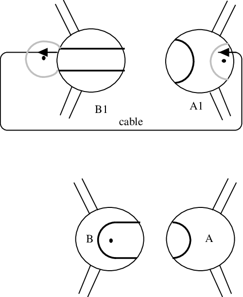 cable
cable
We can formalize this example as follows:
Lemma 6.1
Suppose has Seifert part , fibering over the disk with two exceptional fibers. Suppose intersects as in the parallel annuli case (that is, consists of two essential parallel annuli) and the region between the annuli lies in , say. Then can be cabled into to get a splitting surface intersecting as in the single annulus case. Moreover in there is an annulus with one end a core of the annulus and other end a curve on which is longitudinal in .
Dually, suppose intersects as in the single annulus case and in there is an annulus with one end a core of and other end a curve on which is longitudinal in . Then can be cabled into to get a splitting surface intersecting as in the parallel annulus case.
Proof\quaThe first part is obtained by replacing one of the annuli in with the incident annulus component of . The second part follows from the first by reversing the construction.
In the example preceding the lemma, a spanning annulus as called for in the lemma is one in parallel to . ∎
In each of the seven cases listed above, there is a Seifert part (possibly just a thickened torus in the non-separating torus case) which intersects in annuli and a single complementary component which it intersects in a more complicated surface. Since lies in we know that is atoroidal. It is also acylindrical except possibly for an annulus whose ends in are non-fibered curves and whose complement in is one or two solid tori. That is, could itself be a Seifert manifold over a disk with two exceptional fibers or over an annulus or Möbius band with one exceptional fiber, as long as the fibering doesn’t match the fibering of .
In any case, has the following structure: , where is a properly imbedded surface (either a –punctured sphere or, exactly in the single annulus case, a twice punctured torus) and are each genus two handlebodies. lies in and as the complement of one or two longitudinal curves. In each case where this makes sense (ie, except in the single non-separating torus case), is a fiber of the Seifert manifold on the other side of . (resp. ) can be viewed as the mapping cylinders of maps from to a –complex (resp. ) consisting of one or two annuli in and a single arc in (resp. ) with ends on the annuli. Hence is a product, restricting to a product structure on the annuli . (Here denotes regular neighborhood.) Hence it can be swept out by .
This sweep-out gives us some information about what sort of annuli might be present in .
Lemma 6.2
Suppose contains an essential annulus with neither end parallel to . Then contains an essential annulus or one-sided Möbius band which intersects precisely in two parallel spanning arcs.
Proof\quaConsider how intersects the annulus during the sweep-out of . At the beginning it inevitably intersects in –compressing disks lying in . At the end it intersects in –compressing disks lying in . Nowhere can it intersect it in both, so somewhere it intersects it in neither. (The details are standard and are suppressed.) This means that the intersection of with consists entirely of spanning arcs of . The squares into which are cut by these arcs lie alternately in and . It’s easy to see that all these arcs are parallel in so, we can assemble two of the squares into which is cut, one in and one in , to produce an annulus or one-sided Möbius band which intersects precisely in two arcs. ∎
Let be the annulus or one-sided Möbius band given by the preceding lemma 6.2 and let be the squares in which intersects and respectively. The complement of in is one or two solid tori, depending on whether is separating or not. Moreover the complement of in is also one or two solid tori depending on whether is separating or not, and similarly for . Similarly is one or two annuli. Since these annuli divide each solid torus of into two solid tori, they are longitudinal annuli in the solid torus. These facts give useful information about, for example, the index of the singular fibers, but the crucial point here is that the description is now sufficiently detailed that we have explicitly:
Proposition 6.3
Suppose contains an essential spanning annulus with neither end parallel to . Suppose the annulus is unique up to proper isotopy and is the annulus or one-sided Möbius band given by Lemma 6.2. Then there is an –preserving involution of , defined independently of and a proper isotopy of in so that after the isotopy .
Proof\quaThe proof is left as an exercise. The fixed point set of intersects either
- •
in two points, the centers of each of and or
- •
in two proper arcs orthogonal to the core of or
- •
in the core of ,
depending on the structure of . ∎
Proposition 6.3 is phrased to require a possible isotopy of rather than of , since in it application we will be isotoping two different Heegaard splittings, using as a reference annulus. Also, the proper isotopy of in is not necessarily fixed on , so in fact should be regarded as composed with some Dehn twist along a component (or two) of .
7 Longitudes in genus handlebodies—some technical lemmas
We will need some technical lemmas which detect and place longitudes in a genus two handlebody.
Definition 7.1.
Two curves on a genus two handlebody are separated if they lie on opposite sides of a separating disk in . Two curves are coannular if they constitute the boundary of a properly imbedded annulus in .
Lemma 7.2
Suppose is a genus two handlebody and the disjoint curves divide into two pairs of pants. Suppose that are nonmeridinal curves which are coannular in . Then is either meridinal or it intersects every meridian disk.
Proof\quaSuppose there were a meridian disk disjoint from and consider how intersects the annulus whose boundary is . Assume has been minimized. If then is a separating disk in the handlebody . Then divides into two pairs of pants, so any essential curve in the complement of , eg is parallel either to or a component of . But the latter violates the hypothesis.
If then consider an outermost arc of intersection in . It cuts off a meridian disk of that is disjoint from . Two copies of banded together along the core of in gives a separating disk disjoint from . This reduces the proof to the previous case. ∎
Lemma 7.3
Suppose is a genus two handlebody and the disjoint curves divide into two pairs of pants. Suppose that are nonmeridinal curves which are coannular in . Let be an annulus, with ends denoted , and attach to by identifying to a collar of and to a collar of . Then the resulting manifold is not a genus two handlebody.
Proof\quaIf were a genus two handlebody, then the dual annulus would be a non-separating annulus in . This means that in the handlebody ( again) obtained by cutting open along , both and would be twisted or longitudinal, but in any case each would be disjoint from some meridian disk. But in the case of this would violate Lemma 7.2. ∎
Lemma 7.4
Suppose is a genus two handlebody and the disjoint curves are nonmeridinal curves that divide into two pairs of pants, and , with . Suppose that are separated curves and that is disjoint from some meridian disk. Then one of or is a longitude, and there is a disk which separates and so that .
In particular, if both and are longitudes, then .
Proof\quaLet be the union of three disjoint disks: a disk that separates and , and disjoint meridian disks and which intersect and respectively. Choose this collection and a meridian disk whose boundary is disjoint from , so that, among all such disk collections, is minimal. We can assume that intersects each disk of , since is not parallel to either or . Hence is not parallel to any disk in , so in fact .
By minimality of all components of intersection are proper arcs in . Consider an arc of which is outermost in . Simple counting arguments show that , that the subdisk of cut off by intersects or (say ) in a single point (for the arc is disjoint from ). In particular, is a longitude. Even more, it follows then that as many points of intersection with lie on one side of in as on the other. Since this is true for any outermost arc, it follows that all outermost arcs of in are parallel to in . Furthermore we may as well assume that all outermost disks of cut off by these arcs lie on the same side of , the side containing , since otherwise two could be assembled to give a third meridian disk which would be disjoint from the disks and from the longitude and which would intersect and exactly once. The proof would then follow immediately. (See Figure 23.)

Now consider a disk component of which is “second to outermost”. That is, all but at most one arc of is an outermost arc of intersection with in . To put it another way, is a –gon, where every other side lies in , and of the remaining sides, at least are parallel to in . The last side is perhaps an arc of . (See Figure 24.)

The sides of that lie in and that have both ends on are easy to describe: Since they are disjoint from and are essential in the pair of pants component of on which they lie, each must cross . Moreover, since they are disjoint from , they can’t cross more than once, hence they cross exactly once. Moreover, each must have its ends at opposite ends of , since if any had both ends at the same end of it would follow that and that would force to be parallel to . But even one such arc of , disjoint from and , crossing once and having ends at opposite ends of , could be combined with an outermost disk of with side at to give a meridian disk as described before.

So the only remaining case to consider is , with not parallel to in . So is a square, with one side parallel to and the opposite side, , an arc lying in or . (See Figure 25.) Then simple combinatorial arguments in the pair of pants bounded by and show that , since otherwise and would cross in . With , a simple counting argument shows that cuts off from a disk which can be made disjoint from and intersecting in a single point. The union of this disk and along gives a disk, parallel to a subdisk of cut off by that is disjoint from and and intersects exactly once. It follows that intersects twice, as required. ∎
Lemma 7.5
Suppose is a genus two handlebody and the curves divide into two pairs of pants, and with . Suppose that are separated non-meridinal curves and there is a properly imbedded disk in which intersects in a single point. Then is a longitude, and there is a disk which separates and so that .
In particular, if is also a longitude, then .
Proof\quaSuppose there is a disk that is disjoint from and intersects in a single point. Then is a longitude and it follows from Lemma 7.4 that some disk separating from intersects twice. Using outermost arcs of intersection in , it’s then easy to modify the disk so that is disjoint from . Then must be a meridian curve for the solid torus on the side of that contains . Since intersects in one point, it follows that it also intersects in one point, completing the proof in this case.
Suppose there is a disk that is disjoint from but intersects in one point (so, in fact, is a longitude). By Lemma 7.4 there is a disk that separates and and intersects twice. Choose the pair of disks and so that, among all such disks, is minimal.
Consider an outermost disk cut off by in , so is disjoint from both and . Then lies on the side of containing (since it is disjoint from ) and must intersect at most (hence exactly) once, since it is disjoint from . Thus is also a longitude. ∎
Corollary 7.6
Suppose is a genus two handlebody and the curves divide into two pairs of pants, and with . Suppose that are separated curves. Let be an annulus with ends . Attach to by identifying to a collar of and to a collar of . Suppose the resulting manifold is also a genus two handlebody. Then is a longitude of , and there is a disk which separates and in and which intersects exactly twice. Moreover, if is also a longitude of , then .
Proof\quaLet be the new handlebody, and consider the properly imbedded dual annulus . Since it’s –compressible in , it follows that there is a disk in which intersects in a single point. The result follows from the previous lemma. ∎
Corollary 7.7
Lemma 7.6 remains true if is replaced by any solid torus , attached at and along parallel, essential, non-meridinal annuli in .
The proof is the same, using either attaching annulus at or in place of . ∎
8 Positioning a pair of splittings—the hyperbolike case
A closed, orientable, irreducible –manifold is called hyperbolike if it has infinite fundamental group and contains no immersed essential torus. In the next two sections we will show that any two Heegaard splittings of the same hyperbolike –manifold can be described by some variation of one of the examples in Section 4. As a consequence, the standard involutions of the manifold induced by the two splittings commute.
In this section we will isotope the splitting surfaces and so that they are transverse and so that the curves of intersection and the pieces of the surfaces cut out by them are particularly informative. In the next section, we will move the surfaces so that they are no longer transverse, but rather coincide as completely as possible.
Especially in the latter context, it will be useful to be able to refer easily to the pieces of one splitting surface that lie in the interior of one of the other handlebodies.
Definition 8.1.
Suppose are two Heegaard splittings of . Let denote the closure of . (So if and are transverse, as will not often be true in later discussion, then is just .). Similarly define , and .
We begin with a useful lemma.
Lemma 8.2
Suppose is a genus two Heegaard splitting of a closed hyperbolike manifold and are essential properly imbedded disks in and respectively. Then .
Proof\quaIf then is stabilized and so is either a lens space, or or , but in any case is not hyperbolike. Suppose (so is weakly reducible). If the boundaries of and are parallel in , or one of the boundaries is separating, then is reducible. This means that either is reducible (hence not hyperbolike) or is stabilized, and we have just shown that this is impossible. If the boundaries of and are non-separating and non-parallel then the surface obtained from by doing both compressions simultaneously is a sphere. Moreover contains a separating essential circle of which is compressible on both sides, so again is reducible.
Finally, suppose . Then the union of collar neighborhoods and of and along their two squares of intersection is a solid torus . Denote by (resp. ) the solid torus or pair of tori obtained by compressing along (resp. along ). Then is the union of and , and the annuli of attachment of to and are either longitudinal (if the two points of intersection of and have opposite orientation) or of slope in (if the two points of intersection of and have the same orientation).
So is the union of solid tori along essential annuli in their boundary. It is therefore either reducible or a Seifert manifold. In any case it is not hyperbolike. ∎
Suppose and are two genus two Heegaard splitting of a closed hyperbolike manifold . The two splittings define generic sweep-outs of , as described in [16]. The pair of sweep-outs is paramerized by points in . Points in corresponding to positions where and are not transverse constitute a subcomplex of called the graphic. Complementary components are called regions.
Since the surfaces involved have low genus, we can obtain useful information about their relative positioning even if we allow a more liberal rule than in [16] for labelling regions (that is, positionings in which and are transverse). We label a region (resp. ) if there is a meridian disk for (resp. ) such that . Labels and will be called –labels. Similarly, we label a region (resp. ) if there is a meridian disk for (resp. ) whose boundary is disjoint from . These labels are called –labels.
Suppose that is the collection of curves of that are essential in (resp. ). Then divides (resp. ) into two parts, one lying (except for some inessential parts) in and one in (resp. and ). If the two parts of (resp. ) have even Euler characteristic we say that the positioning is –even (resp. –even). If the two have odd Euler characteristic we say it’s –odd (resp. –odd).
Lemma 8.3
If a region is –odd then its –labels are a subset of the –labels of any adjacent region. Similarly for –odd regions and –labels.
Proof\quaBy construction, we are ignoring curves in which are inessential in , so no component of is a disk. If the region is –odd, then it follows that both parts have Euler characteristic . This implies that, if there is a meridian for disjoint from then in fact some curve in is a meridian of . Since can be pushed into or , this means that both and contain a meridian of .
The effect of moving to an adjacent region in the complement of the graphic is to alter and by adding a band (or a disk) to one and removing it from the other. Clearly adding a band (or disk) doesn’t destroy a curve, such as the meridian, so one copy of the meridian of persists in at least one of or in the new region. ∎
Lemma 8.4
If there are adjacent regions which are both –even (resp. –even) then the –labels (resp. –labels) of one are a subset of the –labels (resp. –labels) of the other. If there are adjacent regions which are each both –even and –even then the set of all labels for one of the regions is a subset of the labels for the other.
Proof\quaSuppose two adjacent regions are both –even. Moving from one region to the other may represent moving across a center tangency, which clearly has no effect on labels, or moving across a saddle tangency. The latter changes the Euler characteristic of and by , so if the parity determined by doesn’t change, the saddle move must have created or destroyed an inessential curve of . This means that one or both ends of the band that is exchanged from to or vice versa, lies on an inessential curve of . If one end lies on an inessential curve, then the move is effectively an isotopy of and so has no effect on the labelling. If both ends lie on the same inessential curve the effect is to add two parallel, possibly essential, curves to . This won’t add a label or , since a meridian lying in the annulus created in previously lay in , but it might destroy some other meridian in , so a label might be deleted. This is the only way in which and labels could change. To summarize: if there is a change in or label it’s to delete a label moving from the first region to the second, and this only happens if the corresponding band has both ends on the same curve of , and that curve is inessential in .
Now consider the situation in if the adjacent regions are also both –even. Moving from the second region to the first we have already seen that the band that’s attached will have its ends on two different curves (the two created in moving from the first to the second region). So no or label can disappear. It follows that the set of labels for the second region is a subset of the set of labels for the first region. ∎
Lemma 8.5
Any region that is –even and –odd (or vice versa) has a label that is also a label of every adjacent region.
Proof\quaIt’s easy to see that and have the same parity: For example, the sum of their parities is the parity of the orientable surface created by doing a double-curve sum of the two surfaces. Furthermore, removing curves of that are inessential in both and does not alter the parity match. So if a region is –even and –odd it follows that at least one curve in is essential in and inessential in (or vice versa), ie, is a meridian of or (or or ). When passing to an adjacent region in the complement of the graphic, a band is added to either or , say the former. Before passing to the new region, move slightly into . Then will still lie in after moving to the adjacent region. ∎
Lemma 8.6
If two adjacent regions have labels and then one of them has both labels and .
Lemma 8.7
No region has both labels and .
Suppose a region has both labels. The meridians are unaffected by removing, by an isotopy, all simple closed curves in which are inessential in both and . The meridians of and which account for the labels must intersect, by 8.2, so they cannot be on opposite sides of . If any curve of is essential in and inessential in then it is a meridian of , say, that can be pushed to lie on the opposite side of from the meridian of , a contradiction. So every curve in is essential in .
Say the meridians of and that are disjoint from both lie in . If any component of is a –parallel annulus, push it across into —this has no effect on the labelling. If possible, –reduce in the complement of . We will assume that no such –reductions are possible, so remains a genus two handlebody—the argument is easier if –reductions can be done. This guarantees that no component of is a meridian disk of so every curve in is also essential in .
Then the boundary of any meridian disk of must intersect , since is strongly irreducible (8.2). In particular, no curve of is a meridian curve for , nor can lie entirely inside of .
Since is compressible yet no boundary component is a meridian of it follows that and a compression of creates a set of incompressible annuli. Since all curves of are essential in both surfaces, one of or , say the former, has . Let be the incompressible annuli in obtained by compressing into . Dually, is obtained from by attaching a tube along an arc dual to the compression disk. It follows from [10, Theorem 2.1] that there is a meridian disk for , isotoped to minimize , so that the arc lies in .
Consider how a distant meridian disk of intersects and how it intersects a compressing disk for . First consider an outermost arc of . Suppose is disjoint from (as we can assume is true if the disk cut off by in lies in ). –compress to via the disk cut off by . This changes an annulus of to a disk . If the tube along were attached to it would violate strong irreducibility of (since is a meridian disk for disjoint from ), so . If is not parallel it is parallel to a meridian disk for disjoint from and if it is parallel then the original annulus was a –parallel annulus in . Either is a contradiction. So we can assume that each outermost arc of in intersects and that the disk in cut off by the outermost arc lies in .
This means that there is a disk in all but at most one of whose boundary arcs in are outermost arcs, and each of these intersects . It is now easy to argue (see [10] for details) that in fact is isotopic in to an arc of which connects two adjacent outermost arcs, ie, is parallel in to a spanning arc of one of the annuli of . But this implies that there is a meridian disk for (the complement of the tube in the annulus of of which has been made a spanning arc) that intersects the compressing disk for dual to in two points. This contradicts 8.2. ∎
Lemma 8.8
There is an unlabelled region.
Proof\quaThe argument is a variant of that in [16]. Combining Lemmas 8.6 and 8.7 we see that adjacent regions can’t have labels and or labels and . So either there is an unlabelled region or there is a vertex whose four adjacent regions are each labelled with one label, appearing in order around the vertex , , , . Then no region is –odd and –even or vice versa, by Lemma 8.5. By Lemma 8.3 the regions labelled and must be –even and those labelled and must be –even, so in fact all must be both –even and –even. But this would contradict Lemma 8.4. ∎
Theorem 8.9
Suppose and are two genus two Heegaard splittings of a closed hyperbolike manifold . Then and can be isotoped in so that each curve in is essential in both and , so that and so that (resp. , , ) is incompressible in (resp. , , ).
Proof\quaConsider the positioning of and represented by an unlabelled region. Curves of intersection that are inessential in both surfaces can be removed by an isotopy without introducing meridians in , , , or , ie, without altering the fact that the configuration is unlabelled. Then all curves of intersection must be essential in both surfaces, for otherwise at least one such curve would be a meridian. If the configuration is –odd (hence also –odd) then we are done.
So suppose the configuration is –even (hence –even). With no loss of generality, assume . Since is a handlebody and the region is unlabelled, is –compressible. Do a –compression. If the boundary compression is on an annulus component of then the result is a disk. It can’t be a meridian disk for , by assumption, so must be –parallel in . Push across the annulus to which it is parallel in . Clearly this does not create a meridian in either (only an annulus has been removed) or in (an annulus has been attached to other annuli). Similarly, if no meridian is created in or .
Suppose . Then after the annuli are pushed across each other, is enlarged, so one might expect that it could contain a meridian curve. But note that if the meridian disk lay in then, after compressing along it one would get a solid torus or two, in which is incompressible. But this is impossible since . Alternatively, if the meridian disk lay in then note that before the annulus is pushed across, the meridian curve intersects only one end of each of the annuli in which have ends on the ends of . But in this case, an easy outermost argument shows that there is a meridian curve in before the annulus is pushed across, another contradiction. So we conclude that nothing is lost by pushing such boundary parallel annuli in across .
Eventually, after these parallel annuli are removed, is –compressible along an arc lying in a non-annular component of . The component of or to which can be –compressed is not an annulus, since contains no meridian curves of . Do the –compression. The result is a positioning of and which is both –odd and –odd and, essentially by 8.3, it remains unlabelled. This configuration is as required. ∎
9 Alignment of and
Lemma 9.1
Suppose and are two genus two Heegaard splitting of a closed manifold , the surfaces , , , and are incompressible in, respectively , , , and . Then the surface –compresses to one of or , and –compresses to the other.
Proof\quaEach surface –compresses in the handlebody in which it lies. With no loss of generality assume that –compresses to . Suppose it also –compresses to . Then since –compresses to one of or , we are done. If fails to –compress to then, symmetrically, fails to –compress to , so it must –compress to . Hence –compresses to . ∎
Definition 9.2.
Suppose and are closed surfaces in a –manifold and (resp. ) is the union of two subsurfaces and (resp. and ) along their common boundary curves. (That is, and similarly for ). Suppose finally that whereas and are transverse. Then we say that and are aligned along .
Lemma 9.3
Suppose are two genus two Heegaard splittings of a hyperbolike closed –manifold. Then the surfaces and can be aligned along a subsurface with in such a way that each component of is essential in all four handlebodies .
Proof\quaFollowing Theorem 8.9, isotope and so that each curve in is essential in both and , so that and so that (resp. , , ) is incompressible in , (resp. , , ). (Since , the last condition is equivalent to saying that each curve in is essential in .) If an annulus component of , say, is parallel to an annulus component of , say, then one can be pushed across the other without affecting these hypotheses. So we can assume that no component of any surface , , , and is a –parallel annulus in the handlebody in which it lies. Then, moreover, any –compression of , if it –compresses an annulus of , would create a compressing disk for either or , contradicting the hypothesis. So we can assume that any –compression of any surface is on the unique component whose Euler characteristic is .
Now apply Lemma 9.1 to find a disk that –compresses to one of or , say , and a disk that –compresses to . The boundaries of the disks and lie on different surfaces so the disks can be made disjoint.
The curve is the union of two arcs, and . A collar of is a –ball whose boundary is the union of two disks parallel to and a collar of each of and in and respectively. The –ball can be used to define an isotopy of that replaces a collar neighborhood of with the union of the disks and the collar of . After this isotopy (and the kinking of collars of the curve(s) of on which the ends of lie), and will be aligned along an essential surface with . Repeat the process on . ∎
Theorem 9.4
Suppose are two genus two Heegaard splittings of a hyperbolike closed –manifold. Then the splittings are both some variation of one of the examples of Section 4. In particular, and commute.
Proof\quaFollowing 9.3, we assume that the surfaces and are aligned along a subsurface with , and each component of is essential in all four handlebodies . We may further assume that no component of is an annulus, for any such annulus could be removed by a small isotopy of the surfaces, perhaps creating a curve of transverse intersection. We further assume that has been minimized by isotopy rel . Then and all consist of incompressible annuli. Any of these annuli that is –parallel in the handlebody in which it lies could be removed by an isotopy (possibly adding it to or ), so in fact all these annuli are essential.
According to 5.2 the ends of in can be isotoped to lie parallel to (at most) two essential non-separating simple closed curves in , and similarly for . Since ends of and can’t cross, there are (at most) three simple closed curves in , decomposing into two pairs of pants, so that any component of is parallel to one of the three curves. Moreover, if all three curves are ends of annuli of then the number of annuli cannot be high, because of the following “Rule of Three”:
Lemma 9.5
If three or more ends of are parallel in then at least one must attach to an end of a curve in . In particular, if has three or more ends at each of two of the curves , then all ends of must also be parallel to those two curves.
Proof\quaImmediate. (See Figure 26.) ∎

We now consider the possibilities:
Case 1\qua
Consider the annuli in the context of Lemma 5.6. By the Rule of Three (Lemma 9.5) and the fact that is separating, or . So either is a single annulus with both ends parallel to the same curve in , or two annuli, one with both ends at and the other with both ends at , or two annuli, each with one end at and one at . In the first two cases, since is essential in , and differ by a cabling into , either on one longitude (example 4.1, Variation 1. See Figure 27) or on two longitudes (example 4.2, Varation 1, with one Dehn surgery done at each site; see Figure 28.)


If is a pair of annuli, each with one end at and one at then the annuli are non-separating. The annuli may both be longitudinal (hence parallel) in . Then the splittings appear as 4.4, Variation 1 (when the are longitudes of as well; see Figure 29) or Variation 2, with the Dehn surgery curve in one of (when the are twisted in ; see Figure 30). The annuli could be twisted and not parallel, so that lying between them is a solid torus on which their cores are torus knots. (See Figure 31.) This is 4.4, Variation 2, with Dehn surgery in . Or they could be twisted and parallel, corresponding to the same Variation but with Dehn surgery in one of . Note that Variations and don’t arise, since is hyperbolike.


Case 2\qua and are both non-empty and the end of each curve in is parallel to one of or .
If at least one annulus in each of or is non-separating, then together they would give a non-separating, hence essential, torus in . This contradicts our assumption that is hyperbolike. So we may as well assume that each annulus in is separating. Hence the ends of are twisted in . They cannot then be twisted in , since is hyperbolike, so is a collection of parallel non-separating longitudinal annuli in .
If has ends at both and (as happens automatically if has more than two components) then both curves are twisted in . Attach a non-separating annulus in with ends at and to the torus (or tori) in on which the are twisted. The boundary of the thickened result would exhibit a Seifert manifold in , again contradicting the assumption that is hyperbolike. We conclude that has exactly two components and that has ends only at , say.
If there were more than two annuli in (hence more than four ends of ) there would have to be more than two ends of at , so we conclude that is made up of one or two annuli. If it’s two annuli, necessarily separating and parallel in , then the relation between and can be seen as follows (See Figure 32): In 4.4, Variation 2 let be the splitting given there with Dehn surgery curve in and be the same splitting given there but with Dehn surgery curve in . To view these simultaneously as splittings of the same manifold , of course, the Dehn surgery curve has to be moved from to , dragging some annuli along, until the splitting surfaces and intersect as described.
 drag
drag
If is a single annulus, it must have one end on and one end on an end of , and the annulus is twisted in . The initial splitting by is as in Example 4.4 Variation 1 (), with a Dehn surgery curve lying in , say. If the splitting is altered by first putting the Dehn surgery curve in (yielding the same manifold ), then altering as in Example 4.4 (ie, considering where ) and then dragging the Dehn surgery curve from to , pushing before it an annulus from the –punctured sphere along which and are identified, we get the splitting surface , intersecting as required. (See Figure 33.)
 drag
drag
Case 3\quaSome end component(s) of or lie parallel to each of ,
Then one of the , say , is parallel only to ends of , and at most (hence exactly) two of them. Another, say , is parallel only to ends of (again exactly two).
Subcase a\quaNo ends of , say, are parallel to .
Then all ends of are parallel to and some ends of are parallel to and some to . So, by the Rule of Three (Lemma 9.5), is a single separating annulus with ends at and is either a pair of separating annuli, one each with ends at and , or a pair of non-separating annuli, each having one end at and one end at . (See Figures 34 and 35.) It follows that when is cut open along the component that contains is a genus two handlebody in which the cores of the annuli appear as separated curves (at least one a longitude), and is a longitude not parallel to either (since splits into handlebodies). Then the technical Lemma 7.4 ( here becomes there) precisely places with respect to the annuli. In particular, if the are separating, (so the argument is precisely symmetric moving from back to ), the splitting is given in Example 4.1, Variant 2. If the are non-separating, the splitting is given in Example 4.4, Variation 5 (if and are not twisted in any of the handlebodies) or Variation 6, with one Dehn surgery curve appropriately placed (if the curves or are twisted in a handlebody).
 on (actual)in (schematic) in (schematic)
 on (actual)in (schematics)detail
Subcase b\quaEnds of both and are parallel to .
The curve can be twisted in at most one of and , so assume that is not twisted in . By 5.6 this means that is a pair of parallel annuli running between longitudes and of .
has two ends at and, as in Case 2, either or ends at . If the annuli are separating and there are ends of at then the cores of the two annuli whose ends are at cobound an annulus in . It follows from 7.2 that any twisted or longitudinal curve in must be parallel to one of these cores. But that would make the core of the annulus in at parallel to one of these cores, hence parallel to or in . Since this is impossible, the case does not arise.
Suppose the annuli in are separating and there are two ends of at . Then consists of two separating annuli, which has both ends at and which has both ends at . The situation is analogous to the last example in Case 2 above, variation 2, with Dehn surgery curve in when is attached to , and in when is attached to . But the presence of adds the additional complexity of Variation 6: is simultaneously moved from to .
If the annuli in are not all separating, and has four ends at then consists of a pair of non-separating annuli with ends at and and a single separating annulus with ends at . Much as in the other case when there were ends at this leads to a contradiction, this time with Lemma 7.3. (See Figure 36.)
 to
to
The final possibility is that the annuli in are not all separating, and has two ends at . Then consists of a pair of non-separating annuli with ends at and . (See Figure 37).
 to to Schematic in Schematic in Schematic of
We will show that this case, too, cannot arise, for if it did:
Claim\quaThen is a Seifert manifold.
Proof of claim\quaSuppose, with no loss of generality, that the (solid torus) region between the annuli in lies in . Then is a genus two handlebody in which the two annuli , have cores , which are separated curves on the boundary. is obtained from by attaching the region that lies between the annuli . One end of is attached to a curve which is parallel in to and in to say. The other end is attached at . It follows from 7.6 that is longitudinal in , and crosses exactly twice a disk that separates and . Notice that is obtained from by attaching a thickened annulus with ends at and . So is a non-separating meridian disk for .
Cut open along to get a solid torus containing and remove from this solid torus all but a collar of the boundary. That is, remove a solid torus whose complement in consists of a collar of to which a –handle, with cocore , is attached. Note that the two annuli intersect in four parallel spanning annuli. Let denote the slope of their ends on .
We will show that is a Seifert manifold. In fact, we will show that fibers over the circle with fiber the three–punctured sphere (ie, the pair of pants) and this suffices. Then a Seifert manifold structure on will be obtained by filling in the solid torus .
Another way to view the compression body is to begin with and attach to it a genus two handlebody by attaching collars of two separated longitudes to two annuli in . The annuli have slope . Note that whereas may be twisted in , we’ve obtained by removing a solid torus so large it contains any cable space, so the attachment circle is indeed longitudinal in . Now when is attached to , one end is attached to along a curve parallel to and the other end is attached along the curve which crosses twice. Then by Lemma 7.6, is a genus two handlebody homeomorphic to , where is a pair of pants whose boundary is the triple of curves . The upshot is that can be viewed as with attached by identifying each of with different parallel annuli on . Each annulus has slope .
What remains of is the genus two handlebody . When this is attached along its entire boundary, it’s easy to see that the three annuli remaining on are identified with annuli corresponding to two distinct separated longitudes in (both parallel to in ) and an annulus whose core is . The fact that is constructed by attaching to the handlebody along and means (see Lemma 7.7) that can be viewed as , where is a pair of pants with the three curves . The upshot is that adding in is the same as attaching by identifying with the remaining annuli of and then the rest of the boundary, , with . But the union of and fibers over the circle with fiber a pair of pants. It’s easy to show then that this manifold is also Seifert fibered by circles transverse to the pair of pants, with a generic fiber running through each of and exactly three times and, in crossing a curve with slope exactly once. The base is a disk and there are two exceptional fibers, each of type .
Now is created from the Seifert manifold just described by filling in a solid torus along its boundary, namely the solid torus that was removed from at the beginning. The result is either a Seifert manifold (if the filling slope differs from that of the fiber) or a reducible manifold, if the filling slope is that of the fiber. In any case, is not hyperbolic. ∎
10 Heegaard splittings when tori are present
Suppose is a closed orientable irreducible –manifold of Heegaard genus two, is not itself a Seifert manifold, and contains an essential torus. Following Section 6, let denote the collection of tori that constitute the canonical tori of . The discussion of Section 6 shows that a genus two Heegaard splitting can be isotoped to intersect so that there is exactly one component (here to be denoted ) of which contains a non-annular part of . Moreover, is a Seifert manifold with at most two components, each of which intersects in fibered annuli. (More is shown there about ). is atoroidal, but could perhaps be a Seifert manifold over a disk with two exceptional fibers or over an annulus or Möbius band with one exceptional fiber, as long as the fibering doesn’t match a fibering of . As in Section 6 we let and let have spines and .
Consider how two different such splittings compare. One possibility is
Example 10.1.
and .
Then in each of and there are essential annuli whose slopes differ from those of the Seifert fibering and respectively. Exploiting Lemma 6.2 and Proposition 6.3 we can write down explicit and simple descriptions of all variations possible here and deduce that, for these two splittings, the commutator can be obtained by Dehn twisting around the unique essential torus .
So henceforth we will assume that and and revert to and as notation. Then , where the splitting surface , the handlebodies and the spines and are defined analogously to and .
Theorem 10.2
Suppose are two non-isotopic genus two Heegaard splittings of an irreducible orientable closed –manifold . Suppose contains an essential torus. Then either the splittings are isotopic, or the relation between the Heegaard splittings is described in one of the variations of one of the examples in Section 4 or in Example 10.1. In particular, the commutator can be obtained by Dehn twists around essential tori in , and the two splittings become equivalent after a single stabilization.
Proof\quaIsotope and so that they each intersect the canonical tori of as described in (possibly different cases of) Section 6, and continue with the same notation. There are two possibilities:
Case 1\qua and have the same slope on each component of .
Then the annuli in and can be chosen to overlap so that their complements in are disjoint. This means that during the sweep-outs of and determined by and respectively, . (See the discussion preceding 6.2 for a description of the sweepout). In particular, the generic intersection of and during the sweepout consists of closed curves. Apply the argument of Sections 8 and 9 almost verbatim to the two sweep-outs. The upshot is a positioning of and so that they are aligned except along some collection of subannuli. That is, and consist of incompressible annuli in and respectively and none of these is parallel in or to a subannulus of .
Consider first of all the case in which and are both –punctured spheres, so any incompressible annulus with boundary disjoint from is –parallel. (This excludes only the case when fibers over the circle with two exceptional fibers and either or intersects as in the single annulus case.) Then and consist entirely of annuli parallel to one of the two annuli in (resp. ). It’s easy to see that these can be removed by an isotopy of which slides around . Thus, after an isotopy of which may move the boundary of , we can make and coincide. Such an isotopy is equivalent to Dehn twists around tori in . The fibered annuli and may also differ within , but can be made to coincide by Dehn twists around essential tori in .
Suppose now that and are both twice–punctured tori. This can arise when fibers over the disk with two exceptional fibers, and both and intersect as in the single annulus case. Then more complicated essential annuli and can occur. In any of , say , essential annuli with boundaries disjoint from can be of two types: parallel annuli non-separating in , each with one end parallel to and the other parallel to a curve ; or parallel separating annuli, both ends parallel to the same single twisted curve . (See Figure 38.)

Since is the set of canonical tori of , there is no essential torus in , nor is there an essential annulus with end having the slope of (). It follows that one of or is empty. For if both and were non-empty and separating, then copies of each could be matched up along their boundaries in to create an essential separating torus in . If both were non-separating, then their ends could be matched up to create an essential non-separating torus in . If were separating and were non-separating (or vice versa), then an annulus of attached to two annuli in , each with their other end on , would give an essential annulus in with slope the fiber of .
So we may assume is empty, and so consists of one separating or two parallel and non-separating annuli. If is a single separating annulus then the splittings are completely described by Example 4.2 Variation 1, with three Dehn surgery curves. One pair produces the other cables into to produce and vice versa.
Suppose consists of two parallel non-separating annuli and suppose that the region between the parallel annuli of lies in , say. Then can be viewed as , where comprises two opposite annuli in the boundary and the other pair of opposite annuli is . Since the annuli are –compressible in it follows that, viewed in , one of the annuli is longitudinal in . Similarly, one of the annuli in is longitudinal in . This suffices to characterise the two splittings as those of Example 4.4 Variation 3, with one of the Dehn surgery curves placed in one of and the other in one of .
Finally, suppose that say, is a –punctured sphere, and is a twice–punctured torus. This means that fibers over the disk with two exceptional fibers; that intersects as in the parallel annuli case; and that intersects as in the single annulus case. Then the argument is a mix of earlier ideas: Once again, after an isotopy of on we can ensure that the annuli in which are not aligned with are not contained in collars of and, in and , these annuli are parallel to the annuli and/or respectively. It follows that (that is, the part of that is aligned with ) is a single –punctured sphere. It follows then that the complement of is a single collection of parallel annuli. Since has two more boundary components than the annuli of not aligned with include collars of exactly two components of . Since no component of is an annulus, it follows that in fact is aligned with except for a single annulus, lying in say. That annulus cuts off collars of two components of , which are the only parts of not aligned with . Put another way: is obtained from by attaching a copy of an annulus component of . Then the setting is exactly as in Lemma 6.1 and preceding. In particular, both splittings are described in 4.4 Variation 3.
Case 2\qua and have different slopes on some component of .
Then is the neighborhood of either a one-sided Klein bottle or a non-separating torus, for otherwise the slope of and must be that of the unique Seifert fibering of . We will concentrate on the latter, for the proof in the former, more specialized, case is similar but easier: A combinatorial proof comparing and , much as in the non-separating torus case below, shows that there is an essential annulus in , so is in fact a Seifert piece attached to , but the fibers do not match. This is Example 10.1.
The argument when is the neighborhood of a non-separating torus will eventually bear a striking resemblance to the hyperbolic case, Section 8.
is the manifold obtained by cutting open along the non-separating torus . consists of two copies of , which we denote . We will denote by (and similarly for ).
Subcase 2a\qua.
Then is the mapping cylinder of a torus. It is shown in [18] (more detailed argument relevant here can be found also in [8]) that the only such mapping cylinders allowing a genus two splittings are those with monodromy of the form
If, for example, is the genus two splitting, then with respect to the coordinates for which is the monodromy, the slope of is . Hence, when we consider both splittings and , it follows that there is an automorphism of the torus that carries the slope of to that of and this automorphism must commute with . If it is easy to check that the matrix of such an automorphism is a power of . It follows that the original splitting can be “spun” around the mapping cylinder until the slopes of and coincide, and so, as above, and are isotopic. (See [8] for more detailed explanation.)
If then is a solvmanifold, whose Heegaard splittings are described in [8]: With precisely two exceptions, each solvmanifold has exactly one isotopy class of irreducible Heegaard splittings (sometimes genus two, sometimes genus three). The two exceptions, corresponding to the case , each have exactly two genus two splittings, for which the associated standard involutions commute, as desired.
Subcase 2b\qua contains an essential spanning annulus
That is, contains an essential annulus with one end on each of . These ends are denoted . Note that if contains two essential spanning annuli of different slopes then, since is irreducible, and we are done by the previous subcase. So we may as well assume that contains a unique (up to proper isotopy) essential spanning annulus .
Lemma 10.3
Neither end of is parallel to (or ).
Proof\quaIf both ends are parallel to , then, arguing as in 6.2, we can arrange that consists of essential closed curves, parallel to the core of . Then isotope to minimize the number of curves; the result is that can be made disjoint from and so lies entirely in or . But this would imply that or contained an essential torus, obtained by isotoping the two curves so that they coincide in . But a handlebody does not contain an essential torus.
If one end of is parallel to and the other end is not, then the involution , which interchanges and , carries to a second spanning annulus in whose slope at each end differs from that of , contradicting our hypothesis that contains a unique essential spanning annulus ∎
Lemma 10.4
does not contain two disjoint arcs and , the former boundary compressing via a disk in and the latter via a disk in . (Similarly for .)
Proof\quaSuppose such curves existed. The ends of lie on . A –compression of along changes it to a pair of pants with one boundary component an inessential circle in . It follows that any essential arc in that is disjoint from and which has both ends on will –compress via a disk in . In particular, also has both ends on . (See Figure 39.) Then simultaneous –compressions on both and give two parallel spanning annuli in . Their ends on have slope perpendicular to that of and on they have slope parallel to . The result then follows from Lemma 10.3. ∎

Following Lemmas 6.2 and 10.3, we can assume that and each intersect in pairs of spanning arcs of . These pairs of arcs can be made disjoint by a proper isotopy of, say, . As noted in the remarks following Proposition 6.3, since we only seek to understand the involutions up to Dehn twists along , we may allow proper isotopies in that are not fixed on . Then, following Proposition 6.3, the involutions and preserve as well as , and induce the standard involution on the solid torus . Of the three possibilities for such an annulus preserving involution of (see the proof of Proposition 6.3) only one sends each boundary component of to itself, as do and . Hence these products coincide with that involution. This implies that the involutions and commute. This implies that and commute, up to Dehn twists along . ∎
Subcase 2c\qua contains no essential spanning annulus.
This case closely parallels that of Section 8, so some of it will just be sketched. We consider the square parameterizing the sweep-outs by and . We label any region in which the two surfaces are transverse with label if there is a meridian disk of whose boundary lies entirely in or if there is an arc component of which –compresses to via a disk in . Similarly apply labels , , and . Labels and (or and ) can’t appear on the same or adjacent regions, in part by Lemma 10.4. So there will be regions with no labels at all.
Consider how appears in an unlabelled region. We can think of the intersection arcs in as a graph whose edges are the arcs of intersection and whose fat vertices are disks filling in the four boundary components of . Two of these vertices, and lie on and two of them and lie on . (See Figure 40.) Similar remarks hold for the graph which describes the arcs of intersection in . Label the vertices in this graph by , , and in a similar fashion.

The valence of each vertex is , where and are the slopes of and in respectively. Since the region has no labels, it follows that there are no trivial loops in or , hence no loops at all. No loops in means that any edge in has one end in one of , and the other end in one of and . (An orientation parity argument is used here.) That is, each edge has one end on a vertex and one end on a vertex, in fact in both graphs. If three or more edges are parallel in say, then the bigons lying between them can be assembled to give a spanning annulus in , contradicting our hypothesis. So we may as well assume that , so each vertex has valence 2.
Now restrict attention to those regions of which are unlabelled. In positionings corresponding to these regions, and are bipartite graphs, so each face has an even number of edges. For each face in or , define the index to be
The sum of the indices of all faces in or is . If the sum of the indices of all faces in (hence also ) is odd (resp. even) we say the positioning is –odd (resp. –even), and similarly for . Since there are no loops in either graph, and the valence of each vertex is , to say a position is –odd is equivalent to saying that both and are disks with four edges. (See Figure 41.) Examination of the few combinatorial possibilities shows that –odd is equivalent to –odd, so we will refer to unlabelled regions as either odd or even. Regions which already have labels are neither even nor odd. Note that a bigon in lying in corresponds to a properly imbedded square so that (resp. ) is an edge of running between (resp. ), and and are spanning arcs of the annuli , one arc in each. Such a square (with two sides spanning the annuli and the other two essential arcs in ) is called a spanning square in . No side of a spanning square in can be isotopic to a side of a spanning square in , for otherwise the two squares could be assembled to give a spanning annulus, contradicting our hypothesis.

Expand the rules for labelling, much as in Section 8, to include the label if there is an arc in which –compresses to via a –compressing disk in , and similarly for the other three labels . (The difference between and is that for the label the –compressing arc needs to be an arc of whereas for label it only needs to lie in .) The labels (resp. will be called –labels (resp. –labels.)
Lemma 10.5
A previously unlabelled region adjacent to a region that has label now has label . Any region adjacent to a region that has only label either itself has label or it is even and has label . Similarly for labels .
Proof\quaThe move from the region with label to the adjacent region corresponds to a band move. The band itself is in a face, and hence is disjoint from the edge of that –compresses in . (See Figure 42.) So the –compressing disk persists even after the band move, though its edge in is no longer in the graph. Thus if the adjacent region had previously been unlabelled it now gets label .

If the original region has only label (and not label or ) then must contain two –compressing disks, one with edge in running from to and the other with edge running from to . A band move that destroys both edges would result in an even region and so one labelled . Otherwise one of the edges persists and the label remains. ∎
Lemma 10.6
Any even region has two primed labels. Adjacent regions cannot both be even. If a region is odd then its labels are a subset (possibly with primes removed) of the labels of any adjacent region.
Proof\quaA region that is even corresponds to a positioning where in there are exactly two edges running between and two between . The resulting bigons lie either both in or both in , say the former. (See Figure 43.) Then intersects only in two parallel spanning squares, so –compresses to in the complement of , forcing the label . A dual argument works from to give a label or .

The band move in corresponding to a move to an adjacent region creates either a loop, an edge corresponding to a loop in (eg an edge with one end on each of and ) or a positioning that is odd. The former two possibilities would have given the corresponding region unprimed labels, so it couldn’t be even.
Consider a positioning corresponding to an odd region and, say, is a label. That is, suppose an arc in , say, –compresses through to . Then the arc has an end on each of and , say. (See Figure 44.) If one performed this –compression one would see that there is also an arc in with ends on and that –compresses through . One of these two arcs will persist in any adjacent region of the graphic, since the corresponding change of positioning of with respect to is via a band move in either (so the second one persists) or (so the first persists). ∎

Lemma 10.7
In a positioning corresponding to an even region, with label , there is a properly imbedded square so that (resp. ) is parallel to an edge of running between (resp. ), and and are spanning arcs of the annuli , one arc in each. Similarly for labels .
Proof\quaSince the label is , there is a –compressing disk for , lying in , one of whose sides is a spanning arc of the annulus , say, and the other side is in but disjoint from the arcs . If one performed this –compression one would see that there is also a –compressing disk for , lying in , one of whose sides is a spanning arc of the annulus and the other side is also in but disjoint from the arcs . Piping these disks together in gives the required square. (See Figure 45.) ∎
 pipe
pipe
Lemma 10.8
No region can be labelled both and or both and . Similarly for labels .
Proof\quaIf both labels and occur then there would be a spanning annulus. If both labels and occur and the region is even, then 10.7 shows how to construct squares in both and which assemble to give a spanning annulus. If the region is odd, then note that in each of the two faces of there is only one isotopy class of arcs with one end point on each of and . (See Figure 46.) It follows that the boundary compressing disks in and either are disjoint or would assemble to make a compressing disk for . The latter violates the hypothesis and the former would create a spanning annulus, contradicting our hypothesis. ∎

Lemma 10.9
No two adjacent regions can be labelled so that one has label or and the other has label one of or . Similarly for labels .
Proof\quaIf adjacent regions are labelled and then in fact one can find disjoint –compressing disks for , one of them in and the other in , contradicting 10.4.
If adjacent regions are labelled and , then by 10.6 one is odd and so one has both labels. This contradicts 10.8.
If a region labelled is adjacent to one labelled then by 10.6 and 10.8, the region labelled must be even. The label on the adjacent region forces, by 10.5, the label onto the region labelled . This again contradicts 10.8. ∎
Lemma 10.10
There is an unlabelled region.
Proof\quaFollowing 10.8 and 10.9, the alternative is that there is a vertex whose four adjacent regions are each labelled with one label, appearing in order around the vertex: or , or , or , or . It follows immediately from 10.6 that no region is odd and no two adjacent regions are even, so at least one of the labels is not primed. The labelling then contradicts 10.5. ∎
To complete the proof of Theorem 10.2 begin with the positioning of and that corresponds to an unlabelled, necessarily odd, region. As in 9.3 one can align and , first pushing arcs in the quadrilaterals and (say) together and arcs in the quadrilaterals and together. The result is that and are aligned except along a set of bigons, since (essentially by 10.5) no loops can be formed in either graph by a band move of across . If two bigons were parallel there would be a spanning annulus, contradicting our hypothesis. So, after the alignment, there are exactly four bigons in , one for each possible way of connecting a vertex or with or . Similarly, there are exactly four bigons in , one for each possible way of connecting a vertex or with or . Each bigon corresponds to a spanning square. (See Figure 47.) The picture is now so explicit that and can be recognized as Variation 3 of Example 4.3. ∎

References
- [1] J Birman, F Gonzalez-Acuna, J M Montesinos, Heegaard splittings of prime –manifolds are not unique, Mich. Math. J. 23 (1976) 97–103
- [2] J Birman, M Hilden, Heegaard splittings of branched coverings of , Trans. Amer. Math. Soc. 213 (1975) 315–352
- [3] M Boileau, D J Collins, H Zieschang, Genus 2 Heegaard decompositions of small Seifert manifolds, Ann. Inst. Fourier, 41 (1991) 1005–1024.
- [4] M Boileau, J-P Otal, Groupes des difféotopies de certaines variétés de Seifert, C. R. Acad. Sci. Paris, 303-I (1986) 19–22
- [5] F Bonahon, Diffeotopies des espaces lenticulaires, Topology, 22 (1983) 305–314
- [6] F Bonahon, J-P Otal, Scindements de Heegaard des espaces lenticulaires, Ann. scient. Éc. Norm. Sup. 16 (1983) 451–466
- [7] A Casson, C McA Gordon, Reducing Heegaard splittings, Topology and its applications, 27 (1987) 275–283
- [8] D Cooper, M Scharlemann, The structure of a solvmanifold’s Heegaard splittings, to appear
- [9] C Hodgson, H Rubinstein, Involutions and isotopies of lens spaces, from: “Knot theory and manifolds”, Lecture Notes in Mathematics 1144, Springer (1985) 60–96
- [10] M Jones, M Scharlemann, How strongly irreducible Heegaard splittings intersect handlebodies, to appear
- [11] W Jaco, Lectures on three–manifold topology, Regional Conference series in Mathematics, no. 43, AMS (1980)
- [12] T Kobayashi, Structures of Haken manifolds with Heegaard splittings of genus two, Osaka J. of Math. 21 (1984) 437–455
- [13] J M Montesinos, Sobre la conjectura de Poincare y los recubridores ramificados sobre un nodo, Tesis, Facultad de Ciencias, Universidad Complutense de Madrid (1972)
- [14] Y Moriah, Heegaard splittings of Seifert fibered spaces, Invent. Math. 91 (1988) 465–481
- [15] Y Moriah, J Schultens, Irreducible Heegaard splittings of Seifert fibered spaces are either vertical or horizontal, Topology, 37 (1998) 1089–1112
- [16] H Rubinstein, M Scharlemann, Comparing Heegaard splittings of non-Haken 3–manifolds, Topology, 35 (1997) 1005–1026
- [17] M Scharlemann, Heegaard splittings of compact –manifolds, from: “Handbook of Geometric Topology”, (R Daverman and R Sher, editors), Elsevier (to appear)
- [18] M Takahashi, M Ochiai, Heegaard diagrams of torus bundles over , Commentarii Math. Univ. Sancti Pauli, 31 (1982) 63–69
- [19] O Viro, Linkings, 2–sheeted coverings and braids, Mat. Sb. (N. S.), 87(129) (1972), 216–228, English translation; Math. USSR-Sb. 16 (1972) 223–226