The Dimension of the Brownian Frontier is Greater Than 1.
Christopher J. Bishop11 1 Supported in part by NSF grant # DMS 9204092 and by an Alfred P. Sloan Foundation Fellowship., Peter W. Jones22 2 Research partially supported by NSF grant # DMS 9213595.,
Robin Pemantle33 3 Research supported in part by National Science Foundation grant # DMS 9300191, by a Sloan Foundation Fellowship, and by a Presidential Faculty Fellowship. and Yuval Peres44 4 Research partially supported by NSF grant # DMS-9404391.
State University of New York, Yale University,
University of
Wisconsin, and University of California.
Abstract
Consider a planar Brownian motion run for finite time. The frontier or “outer boundary” of the path is the boundary of the unbounded component of the complement. Burdzy (1989) showed that the frontier has infinite length. We improve this by showing that the Hausdorff dimension of the frontier is strictly greater than 1. (It has been conjectured that the Brownian frontier has dimension , but this is still open.) The proof uses Jones’s Traveling Salesman Theorem and a self-similar tiling of the plane by fractal tiles known as Gosper Islands.
Keywords: Brownian motion, frontier, outer boundary, Hausdorff dimension, self-similar tiling, traveling salesman
Published in modified form: J. Funct. Anal. 143 (1997), 309–336 Stony Brook IMS Preprint #1995/9 June 1995
1 Introduction
Let be any compact, connected set in the plane. The complement of has one unbounded component and its topological boundary is called the frontier of , denoted . The example we are most interested in is when is the range of a planar Brownian motion run for a finite time (see Figure 1). In this case, Mandelbrot (1982) conjectured that the Hausdorff dimension is . Rigorously, the best proven upper bound on the dimension is by Burdzy and Lawler (1990). Burdzy (1989) proved that has infinite length; our main result improves this to a strict dimension inequality:


Theorem 1.1
Let denote the range of a planar Brownian motion, run until time . There is an such that with probability 1, The Hausdorff dimension is at least . Moreover, with probability 1,
where the inner infimum is over all open sets that intersect .
Remarks: The uniformity in implies that almost surely for any positive random variable (which may depend on the Brownian motion). We also note that our proof shows that the frontier can be replaced in the statement of the theorem by the boundary of any connected component of the complement . (One can also infer this from the statement of the theorem by using conformal invariance of Brownian motion). As explained at the end of Section 6, The result also extends to the frontier of the planar Brownian bridge (which is a closed Jordan curve by Burdzy and Lawler (1990)).
Bishop and Jones (1994) proved that if a compact, connected set is “uniformly wiggly at all scales”, then it has dimension strictly greater than 1. Here we adapt this to a stochastic setting in which the set is likely to be wiggly at each scale, given the behavior at previous scales. The difficulty is in handling statistical dependence.
Definitions: Let be a compact set in the plane with complement , and let . Denote by core the set . Say that the compact set -surrounds if topologically separates core from , i.e., if core is disjoint from the unbounded component of .

Theorem 1.2
Let be the Gosper Island, defined in the next section and illustrated in Figure 2. There exists an absolute constant with the following property. Suppose that , and is a random compact connected subset of the plane such that for all homothetic images of with and in the plane:
| (1) |
where the conditioning is on the -field generated by the random set outside the interior of . Then there is an , depending only on , such that
with probability 1. More generally, for any open intersecting .

Remarks: 1. In fact, the proof in Section
shows that
with probability 1, for any connected component
of and any open intersecting ,
there is a John domain with
closure contained in
, such that
.
2. The constant
will be chosen in the next section to ensure that no “macroscopic”
line segment can be wholly contained within a -neighborhood
of the Gosper Island’s boundary .
The appearance of the Gosper Island might seem strange at this point, but is explained as follows. The hypothesis on that guarantees “wiggliness” should be local to handle dependence (thus it must hold inside each conditioned on ). If -surrounds , or , then cannot intersect core. Having thus controlled inside , away from the boundary of , we must worry about how behaves near boundaries of cells , as these run over a partition of the plane. If a small neighborhood of the union of the boundaries of cells of a fixed size contains no straight line segments of length comparable to , then no significant flatness can be introduced near cell boundaries. To apply the argument with the same constants on every scale, we need a self-similar tiling where tile boundaries have no straight portions; the Gosper Island yields such a tiling.
Proving Theorem 1.2 is the main effort of the paper and is organized as follows. Section 2 summarizes notation and useful facts about the Gosper Island. We also discuss the notion of a Whitney decomposition with respect to these tiles. Section 3 constructs a random tree of Whitney tiles for and reduces Theorem 1.2 to a lower bound on the expected growth rate of the tree, via some general propositions on random trees. In Section 4 we state a variant of Jones’s Traveling Salesman Theorem adapted to the current setting. In Section 5 this theorem is used to derive the required lower bound on the expected growth rate of the “Whitney tree” mentioned above, which then finishes the proof of Theorem 1.2. In Section 6 we verify that the range of planar Brownian motion, killed at an independent exponential time, satisfies the hypothesis of Theorem 1.2; this easily yields Theorem 1.1. Finally, section 7 gives a hypothesis on the random set that is weaker than (1), but still implies the conclusion of Theorem 1.2.
2 Gosper Islands and Whitney tiles
The standard hexagonal tiling of the plane is not self-similar, but can be modified to obtain a self-similar tiling. Replacing each hexagon by the union of seven smaller hexagons (of area that of the original – see Figure 4) yields a new tiling of the plane by -sided polygons; denote by the Hausdorff distance between each of these polygons and the hexagon it approximates. Applying the above operation to each of the seven smaller hexagons yields a -sided polygon with Hausdorff distance from the -sided polygon, which also has translates that tile the plane. Repeating this operation (properly scaled) ad infinitum, we get a sequence of polygonal tilings of the plane, that converge in the Hausdorff metric to a tiling of the plane by translates of a compact connected set called the “Gosper Island” (see Gardner (1976) and Mandelbrot (1982)).


Notation: We normalize to be centered at the origin and have diameter 1. Denote by the set of translates of that form a tiling of the plane (depicted in Figure 6). This tiling is self-similar, i.e., there is a complex number with such that for each tile , the homothetic image is the union of tiles in . (For the tiling by Gosper Islands, .) For each integer , we denote by the scaled tiling , and let . If we say that is a tile of index and write . Every tile is contained in a unique tile of , denoted . Each tile is centrally symmetric about a “center point” ; for any , denote by the expansion of by a factor around .

We record several simple properties of the tiling by Gosper Islands, which will be useful later.
- 1.
There is some minimal distance between any two nonadjacent tiles of .
- 2.
There is an such that any line segment of length must intersect for some . (The existence of follows by a compactness argument from the fact that contains no straight line segments.)
- 3.
The Gosper Island contains an open disk centered at the origin which in turn contains .
- 4.
The blow-up contains for any (see Figure 7).
- 5.
If for neighboring tiles and , then contains . (See Figure 7.)
- 6.
The blow-up is contained in where the union is over all neighbors of of index .
- 7.
The boundary of is a Jordan curve. To see this note that when we replace each segment or length by the three segments of the next generation, they remain within distance of the segment. Thus the limiting arc is within
of the segment. If are consecutive segments of length then , so this shows the limiting arcs corresponding to them are at least distance apart. Thus the boundary of the Gosper Island is a Jordan curve, indeed, is the image of the unit circle under a map satisfying
where .
- 8.
For any , there is a topological annulus with a rectifiable boundary, which separates from the boundary of the Gosper island.
(By the previous property, the interior of is simply connected, so this annulus can be obtained, for instance, by applying the Riemann mapping theorem.)
Definitions: Let be a compact connected subset of the plane. We say that is a Whitney tile for if is disjoint from , but intersects . (See Figure 7.) Let denote the set of Whitney tiles for . This collection is called a Whitney decomposition of , since it decomposes into a countable union of tiles (disjoint except for their boundaries) each with diameter comparable to its distance from . See Figure 8.
A chain of adjacent tiles in such that and for all is called a Whitney chain (see Figure 8). Given , define to be the set of tiles such that there is a Whitney chain with and .
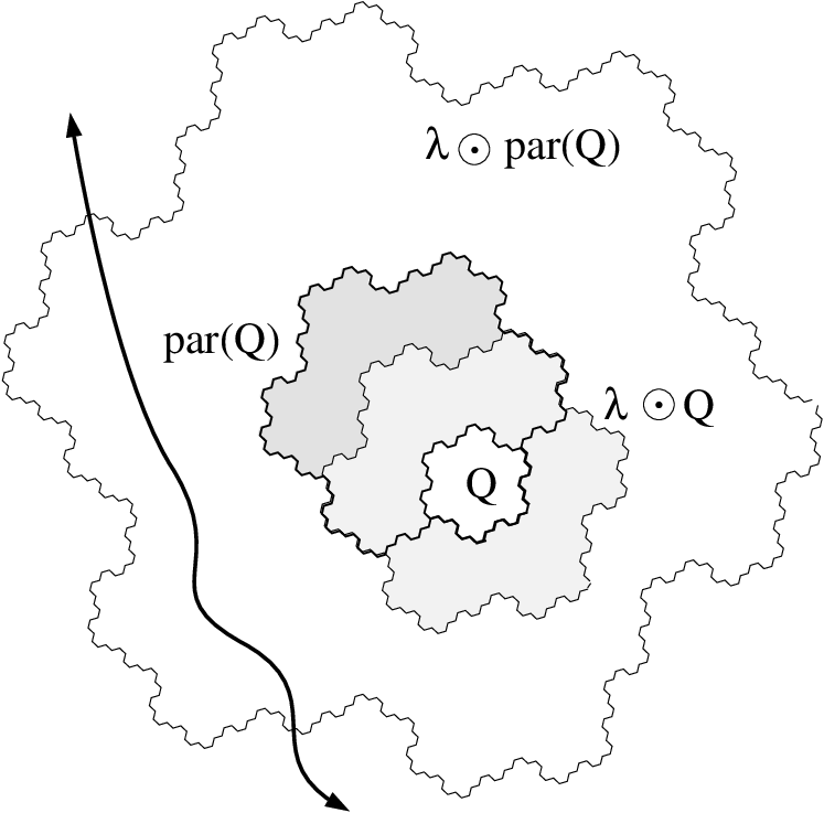

Note the following property of the Whitney decomposition, which holds for any connected component of :
| (2) |
Lemma 2.1
If are adjacent then is 0 or .
Proof: Suppose . Let
be the tile of index that contains ,
and observe that is adjacent to . Then by Property 5
of the Gosper tiling,
and maximality of is violated.
Lemma 2.2
Suppose is a collection of tiles whose union topologically surrounds a smaller Whitney tile where . Then surrounds a a point of .
Proof: The -fold parent of is a tile which is surrounded by . Applying Property 6 inductively shows that the union of for surrounds whatever part of it does not contain. Thus maximality of implies that intersects , and any point of intersection is surrounded by .
Lemma 2.3
Suppose that and that there is a Whitney chain from some larger tile outside to . For any define to be the set . (See Figure 9.) Let
Then is a connected set which topologically separates from . Furthermore, If is a Jordan curve separating from the complement of , then every component of intersecting the domain bounded by also intersects .

Proof: By Lemma 2.1 any path which connects to must hit Whitney tiles of every index larger than . Thus any such path either hits or must leave , proving that separates from . Connectedness follows from the last assertion of the lemma for , so it remains only to prove the last assertion.
Suppose to the contrary that there is a component of which intersects the domain bounded by but is disjoint from itself. The union of all Whitney tiles which are in the unbounded component of and are adjacent to is a connected set. By Lemma 2.1 all of these tiles have index or . By connectedness and Lemma 2.1, they must all have a single index. Suppose they all have index . Since tiles in can be connected to by Whitney chains which don’t cross any tile of index , this means is in a bounded component of the complement of , which contradicts our assumption that could be connected by a Whitney chain to a larger tile outside . Thus the adjacent tiles must all have index . But then by Lemma 2.2 these adjacent tiles must also surround a point of , which implies that is not connected, another contradiction.
The next two lemmas are needed in order to show that if “major portions” of a wall of Whitney tiles can be covered by a thin strip, then must intersect the core of an appropriate tile without -surrounding it; the latter event is controlled by the hypothesis of Theorem 1.2.
Lemma 2.4
Fix and . Let
be any connected set intersecting both
and . Suppose that
is contained in an infinite open strip
of width .
Then there is a tile contained in and
of the same index as , such that
intersects .
Proof: Pick a point and choose connected to inside . By Property 1 of the tiling, the segment has length at least , so by Property 2 of the tiling, there is a tile of the same index as , such that contains some point . By Property 3 and convexity of disks, , and therefore . Observe that , for if not, removing the open disk centered at of radius from the infinite strip would contradict the connectedness of . This observation implies the assertion of the lemma.
Let be any Whitney tile with not containing all of . Let be a circle centered at which separates from . (Such a circle exists by Property 3 of the tiling.) For any positive integer , let be the union of all tiles of index such that intersects the disk bounded by (see Figure 9).
Lemma 2.5
Choose so that . With as above, let be a tile in with such that is contained in the disk bounded by . Suppose that is covered by an open strip of width with . Then there is a tile of the same index as , such that intersects without -surrounding .
Proof: By Lemma 2.3, is connected and therefore satisfies the hypotheses of Lemma 2.4; let be a tile as in the conclusion of that lemma. Since , we can pick a point in . This clearly prevents from -surrounding . For any Whitney tile of index , the blow-up intersects (by Property 4 of the tiling). Since is a union of tiles of index , it follows that
by the choice of . Therefore intersects .
3 A tree of Whitney tiles
Fix a compact, connected , a tile , and a positive integer, . We construct a tree of Whitney tiles. The root of is and the remaining generations of are defined recursively as follows.
Assume has been defined up to generation and for each in , the generation of , define to be the set of tiles with the following properties:
1. ;
2. ;
3. .
Let be a subcollection of which has maximal cardinality among all subcollections for which the expanded tiles are disjoint. By maximality, contains all tiles in and therefore
| (3) |
The children of in are defined to be the collection . Some trivial inductive observations are that , that each is connected to by a Whitney chain, and that the sets are disjoint as runs over any .
Some tree terminology: Let be a countable set.
-
(i) A mapping T from a probability space to the set of trees on the vertex set is measurable with respect to a on , if for any pair , the event is in .
-
(ii) For any tree with vertex set contained in , and any element , define to be null if is not a vertex of , and otherwise let be with the part below removed; more precisely, the vertices of are the vertices of not separated from the root by , and the edges are the edges of spanning pairs of vertices in this smaller vertex set.
For any , let denote the generated by the events for all tiles for which either or the interior of is disjoint from .
Lemma 3.1
On the event , the random variable is measurable with respect to .
Proof: Suppose and consider an event of the form
where and are tiles of index and
respectively,
with .
If and is not disjoint from
, then the edge cannot be in
. If or is
disjoint from then the event that
is an edge of is the union of events witnessed
by particular Whitney chains of tiles, all tiles being either
disjoint from or of index at most
, so the event is measurable with respect to .
The next lemma requires the traveling salesman theorem described in the next section, so its proof is delayed until Section 5.
Lemma 3.2
Assume the random set satisfies the hypotheses of Theorem 1.2. Fix any tile and and let be the random tree . There are constants such that for any tile ,
| (4) |
on the event that , the tile is in , and does not contain . The constants and depend only on .
To prove Theorem 1.2, we also need two general lemmas concerning trees. Define the boundary of the infinite rooted tree to be the set of infinite self-avoiding paths from the root. The next lemma is implicit in Hawkes (1981) and can be found in a stronger form in Lyons (1990). For convenience, we include the short proof.
Lemma 3.3
Let be an infinite rooted tree. Given constants and , put a metric on by
| (5) |
Suppose that independent percolation with parameter is performed on , i.e., each edge of is erased with probability and retained with probability , independently of all other edges. If
then with probability 1, all the connected components of retained edges in are finite.
Proof: It suffices to show that the connected component of the root is finite almost surely. For any vertex of , denote by the number of edges between and the root. By the dimension hypothesis and the definition of the metric on , there must exist cut-sets in for which the -dimensional cut-set sum
is arbitrarily small. But for any cutset , the right-hand side is the expected number of vertices in which are connected to the root after percolation; this expectation bounds the probability that the connected component of the root is infinite.
The next lemma formalizes the notion of a random tree which “stochastically dominates” the family tree of a branching process. We require the analogue of a filtration in our setting.
Definition: Let be a countable set and let be a random tree with vertex set contained in , i.e., is a measurable mapping from some probability space to the set of trees on the vertex set . Say that s on form a tree-filtration if for any and any , the event is -measurable.
Lemma 3.4
Let be a countable set and let be a random tree with vertex set contained in . We assume that is rooted at a fixed . Assume that and a tree-filtration exists such that (defined before Lemma 3.1) is -measurable for each , and the conditional expectation
If every vertex of has at most children and at least children, , then
- 1.
The probability that is infinite is at least , where is the unique fixed point in of the polynomial
(Observe that when .)
- 2.
for any .
- 3.
If is endowed with the metric (5), then with probability at least .
Proof: 1. Let be the size of the generation of . and let denote the -fold iterate of . We claim that for ,
| (6) |
When , convexity of implies that
and the claim follows by taking expectations:
since . For proceed by induction. Let be the number of children of if and zero otherwise, and use the argument from the case to see that on the event (which is an event in ). Giving an arbitrary linear order (denoted “”), we have in particular
for . Since
Taking expectations and applying the induction hypothesis with in place of gives
proving the claim (6).
From (6) we see that , establishing the first conclusion of the lemma.
2. By copying the derivation of (6), inserting an extra conditioning on , one easily verifies that , and the rest of the argument is the same as in the first part.
3. Let be the connected component of the subtree of below after removing each vertex of below independently with probability . For , let solve . We apply the second part of the lemma to conditioned on to see that
for . By Lemma 3.3, the event is contained up to null sets in the event . Thus
since each event conditioned on is in the corresponding . Taking expectations yields
Since for each , this goes to as , proving the last conclusion of the lemma.
Proof of Theorem 1.2: Put a metric on by
Each defines a unique limiting point which is the decreasing limit of the set . If and share exactly edges, then by definition of , the expanded tiles and are disjoint. Since and , it follows from Property 1 of the tiling that
Thus
and since the range of is included in it follows that
| (7) |
From Lemma 3.4 and the conclusion of Lemma 3.2, we see that
| (8) |
with probability 1, on the event that and does not contain . Choose to maximize the RHS of (8). Since the maximum is greater than 1, there is an for which
with probability 1 on this event. Finally, let be any connected component of . By property (2 of the Whitney decomposition, for any open intersecting , there is a tile with , and the theorem follows from (7).
Remark: A planar domain is called a John domain if there is a base point and a constant so that any point can be joined to by a curve so that for any . John domain were introduced by Fritz John in 1961, and some basic facts about them can be found in Näkki and Väisälä (1994).
With the notation of the above proof, if is contained in a component of , choose for every tile in the tree , a Whitney chain leading to from its unique ancestor in the previous generation of the tree. For each tile in this chain, there is an open disk containing it which is contained in (by Property 3 of the tiling). The union of all these open disks as runs over the chosen Whitney chain for and runs over , is a John domain satisfying .
4 The traveling salesman theorem
Given a set in the plane and another bounded plane set , we define
where is the set of all lines intersecting .
Theorem 4.1 (Jones 1990)
If then the length of the shortest connected curve containing is bounded between (universal) constant multiples of
where the sum is over all dyadic squares in the plane and is the union of a 3 by 3 grid of congruent squares with as the central square.
A simpler proof of this Theorem, and an extension to higher dimensions, are given in Okikiolu (1992). The theorem easily implies that the length of any curve which passes within of every point of satisfies
| (9) |
where the sum is over all dyadic squares in the plane with diameter at least . For every set , there is a dyadic square of side length at most for which . Picking for some tile and accordingly, we get
and since each expanded square contains a bounded number of expanded tiles for tiles with , it follows that the length of any curve passing within of every point of satisfies
| (10) |
We require the following corollary, which uses an idea from Bishop and Jones (1994).
Corollary 4.2
Let be a Jordan curve with length denoted and let be a collection of Whitney tiles of index . Let denote and suppose that is connected. Then there is a constant such that the cardinality of is at least
where is the collection of tiles of index at most for which intersects .
Proof: Let be the collection of circles of radius centered at points for . Since neighboring tiles in give rise to intersecting circles in , we see that is connected and passes within of every point of . Furthermore, any connected finite union of closed curves is a closed curve, and hence is a curve of length at most . Combining this with (10) shows that
Since all tiles in have diameter at least , this proves the lemma.
5 Expected offspring in the Whitney tree
Proof of Lemma 3.2: Fix and as in the statement of the lemma and let be any tile in . Let be the circle separating from , which was used in Lemma 2.5. Let be the collection of tiles of index intersecting the disk bounded by . The union of all tiles in is the set defined before Lemma 2.5. We want to show that the expected cardinality of is large. Since the cardinality of is at least times the cardinality of by (3), and is a superset of , it suffices to show that
To do this, we will apply Corollary 4.2 to , so that the set defined in that corollary is the same as defined above.
We will be able to bound from below the summands in Corollary 4.2 for most, but not all, “intermediate-sized” tiles . Pick an integer so that , where is the minimal distance between nonadjacent tiles in . Let be a circle concentric with , with a smaller radius: (see Figure 10).

For , let be the set of tiles such that and intersects the disk bounded by . For any such tile the blow-up is contained in the disk bounded by .
Fix any tile with , where was specified in Lemma 2.5. That lemma implies
| (11) | |||||
where the intersection is over all tiles such that . The set of such tiles for a fixed has cardinality . Enumerating these and multiplying conditional probabilities using the hypotheses of Lemma 3.2 (since the -fields and are contained in ) gives a lower bound of for (11), and implies that
(This is the definition of ). Since is outside , the distance from to is at least , by Property 1 of the tiling. Therefore the distance from to is at least , which is greater than by the choice of . By Lemma 2.3, the union of with all the tiles in is a connected set. Since it intersects both and , it follows that the cardinality of is at least . Thus for each we have
By Corollary 4.2,
Summing gives
which proves the lemma since .
6 The Brownian frontier: Proof of Theorem 1.1
Let denote the law of a planar Brownian motion started at . We use unless indicated explicitly otherwise. Let be a positive random variable, independent of the Brownian motion, which is exponential of mean 1 (i.e., its density is ). We will verify (1) for . by Brownian scaling, this will imply the first assertion of Theorem 1.1.
Notation: for any compact planar set , denote by the first hitting time of , which is almost surely finite if has positive logarithmic capacity. Given , let be a rectifiable closed Jordan curve, which is the exterior boundary of a topological annulus separating from . (Here the constant can be replaced by any constant smaller than the inradius of , and the existence of is guaranteed by Property 8 of the tiling.) For the rest of this section, consider a homothetic image of the Gosper Island , with and in the plane. Also, denote by the image of in . We must obtain estimates which are uniform in the location and scale of , as well as in the structure of the Brownian range outside .
Lemma 6.1
For every ,
| (12) |
Furthermore, there exists such that
| (13) |
Proof: The first estimate is immediate for , and the general case follows by scaling. For the second, observe that by Brownian scaling, is a positive constant depending only on , hence only on . Also, clearly and therefore
Applying (12), lack of memory of exponential variables, and the strong Markov property of Brownian motion at the stopping time , then shows that the left-hand side of (13) is at least a constant multiple of . On the other hand, for any we have . This completes the proof.
Lemma 6.2
There exists such that for any tile , for any and any ,
Proof:
Recall that is a Jordan curve of finite length
separating core from . The Harnack principle (see,
e.g., Bass (1995, Theorem 1.20)) implies
that there is a constant
such that for any
and for any ,
| (14) |
Therefore for any ,
| (15) |
Applying the Harnack inequality (14) with and then invoking the estimate (12) from the previous lemma, we find that the expression (15) is at least , for any . Finally, taking and averaging with respect to using the strong Markov property gives
for any Borel set . This proves the lemma.

Given , we abbreviate and partition the Brownian trajectory into three pieces:
- 1.
Until the first time that the path visits .
Formally, define for , where is shorthand for . - 2.
From time until the next visit to , denoted .
Define for . - 3.
After time .
Denote for .
The idea now is that and determine the Brownian range outside , and has a substantial chance of -surrounding , even when we condition on its endpoints. However, we still have to take the exponential killing into account. Define the random variable
that indicates in which part of the motion the exponential killing occurred. Finally, define
Proposition 6.3
For any there is a constant such that for all homothetic images of with and in the plane:
| (16) |
where the conditioning is on the -field generated by and .
Proof:
On the event , the set
is disjoint from core .
To handle the case , we use the strong Markov property at
time and apply the estimate (13) to .
Denoting
, this gives
This proves (16) on the event .
Only the case remains. By using the strong Markov property at time and applying Lemma 6.2 to , we see that for any ,
In other words,
An application of the strong Markov property
at time shows that this lower bound
is still valid if we insert an additional conditioning on
and on .
Finally, since and
is conditionally independent of
given , this completes the proof of the proposition.
To obtain the uniformity in Theorem 1.1, we will need the following general observation.
Lemma 6.4
Let be any continuous path and let . For any open disk intersecting such that , there is a such that for any , we have
| (17) |
Proof: By hypothesis intersects the unbounded component, . of , so there is a point with and an unbounded curve starting from and contained in . Using the convexity of , we can append to this curve a line-segment connecting to a nearest point on , and thus obtain an unbounded curve starting at and contained in . Choose small enough so that is disjoint from the curve . This gives the right-hand side of (17) for . If we also require that is disjoint from , then the left-hand side of (17) follows from the general fact that
Proof of Theorem 1.1: The random set is completely determined by the variables generating the -field defined in Proposition 6.3, so the proposition implies that satisfies the hypothesis (1) of Theorem 1.2.
Since has the same distribution as , this establishes the first assertion of Theorem 1.1.
For , Let be the event that simultaneously for all open disks that intersect and have rational centers and radii. Theorem 1.2 and Proposition 6.3 give , and we must show that . Denote by the intersection over all positive rational times. Now Brownian scaling and countable additivity imply that , so it suffices to prove that for all . Fix and an open disk that intersects . Since is connected, it must intersect some (random) open disk with rational center and radius such that and . By the previous lemma, there is a rational such that
This implies that , and completes the proof of the theorem.
Finally, we consider the planar Brownian bridge , which may be defined either by conditioning the Brownian path to return to the origin, or by for . For every , the restrictions and have mutually absolutely continuous laws (these laws are measures on the space of continuous maps from to the plane.) Therefore by Theorem 1.1, for every fixed ,
| (18) |
Consider a sequence of annuli of modulus around the origin. The probability that surrounds the origin in is bounded away from 0, so the Blumenthal 0–1 law implies that with probability 1, there is some rational such that (see Burdzy and Lawler (1990)). Thus by (18), with probability 1,
7 Concluding remarks
It can be shown (Krzysztof Burdzy, personal communication) that is almost surely constant; this fact is not required for the arguments in this paper. The conjecture that the Brownian frontier has dimension is related to well-known conjectures concerning self-avoiding random walks, which in turn are a model for long polymer chains. In that context, the exponent first appeared in the non-rigorous considerations of Flory (1949); see also de Gennes (1991).
Theorem 1.2 is stated for general random sets, rather than just Brownian motion, in view of potential applications to the ranges and level-sets of other stochastic processes. Besides the range of Brownian motion, another natural random set that satisfies the hypothesis of Theorem 1.2 is the support of super-Brownian motion, i.e. the intersection of all closed sets that are assigned full measure by this measure-valued diffusion throughout its lifetime. (For the definitions see, e.g., Dawson, Iscoe, and Perkins (1989).) Equivalently, this random set may be characterized as the set of points ever visited by the path-valued process constructed by Le-Gall (1993). (This process is often referred to as “The Brownian snake”.). We are grateful to Steve Evans for enlightening discussions of super-Brownian motion.
To allow for further applications, we state below a variant of Theorem 1.2 which obtains the same conclusions under weaker hypotheses on the random set . We omit the proof, which requires the estimates obtained by Pemantle (1994) for the probability that a Wiener sausage covers a straight line segment.
For any set and any , let denote the set . Say that is -flat inside if there is some line segment of length covered by , having inside with not topologically surrounded by .
Theorem 7.1
Let be the Gosper Island, and let be a random compact connected subset of the plane. Suppose that for some , the following hypothesis on is satisfied, where the supremum is over and in the plane.
| (19) |
Then there is an for which with probability 1.
Remark: The intuition behind the two-part definition of -flatness is that for to be close to straight (thus for to be flat), itself must nearly cover a line segment and this must happen somewhere that is not completely encircled by .
For the special case when is the range of planar Brownian motion, it seems likely that methods directly adapted to this case will yield better estimates for than those obtainable by our methods. Indeed, Gregory Lawler has informed us that immediately after he learned of our Theorem 1.1 (but without seeing its proof), he proved (using completely different methods) that the dimension of the Brownian frontier can be expressed in terms of the “double disconnection exponent” of Brownian motion. This allowed Lawler to deduce that a.s., by invoking recent estimates of Werner (1994) on disconnection exponents. We refer the reader to Lawler’s forthcoming paper for this and several other striking results on the Brownian frontier.
Finally, we note an application to simple random walk on the square lattice . Given a subset of , say that a lattice point is on the outer boundary of if is adjacent to some point in the unbounded component of We remark that using the strong approximation results of Auer (1990) and our construction of the Whitney tree in Section 3, it is easy to derive the following.
Corollary 7.2
Let denote simple random walk on , and let be as in Theorem 1.1. Then for every we have
References
- [1] Auer, P. (1990). Some hitting probabilities of random walks on . In: Berkes, L. Csáki, E. and Révész, P. (eds.) Limit Theorems in Probability and Statistics, North-Holland, 9–25.
- [2] Bass, R. (1995). Probabilistic techniques in analysis. Springer-Verlag, New York.
- [3] Bishop, C.J. and Jones. P.W. (1994). Hausdorff dimension and Kleinian groups. Preprint.
- [4] Burdzy, K. (1989). Geometric properties of -dimensional Brownian paths. Probab. Th. Rel. Fields 81, 485–505.
- [5] Burdzy, K. and Lawler, G.F. (1990). Non-intersection exponents for Brownian paths. Part II: Estimates and applications to a random fractal. Ann. Probab. 18, 981–1009.
- [6] Dawson, D.A., Iscoe, I. and Perkins, E.A. (1989). Super-Brownian motion: Path properties and hitting probabilities. Probab. Th. Rel. Fields 83, 135–205.
- [7] Flory, P. (1949). The configuration of real polymer chains. J. Chem. Phys. 17, 303-310.
- [8] John, F. (1961). Rotation and Strain. Comm. Pure Appl. Math 14, 391–413.
- [9] Gardner, M. (1976). Mathematical games: In which “monster” curves force redefinition of the word “curve”. Scientific American 235, December, 124–134.
- [10] de Gennes, P.-G. (1991). Scaling concepts in polymer physics. Cornell University Press.
- [11] Hawkes, J. (1981). Trees generated by a simple branching process. J. London Math. Soc. 24, 373–384.
- [12] Jones, P.W. (1990). Rectifiable sets and the travelling salesman problem. Invent. Math. 102, 1–15.
- [13] Le-Gall, J.F. (1993). A calss of path-valued Markov processes and its application to superprocesses. Probab. Th. Rel. Fields 95, 25–46.
- [14] Lyons, R. (1990). Random walks and percolation on trees. Ann Probab. 18, 931–958.
- [15] Mandlebrot, B.B. (1982). The Fractal geometry of nature. W. H. Freeman & Co.: New York.
- [16] Näkki, R. and Väisälä, J. (1991). John disks. Expositiones Math. 9, 3–43.
- [17] Okikiolu, K. (1992). Characterizations of rectifiable sets in . J. London Math. Soc. 46, 336–348.
- [18] Pemantle, R. (1994). The probability that Brownian motion almost contains a line segment. Preprint.
- [19] Werner, W. (1994). Some upper bounds of disconnection exponents for two-dimensional Brownian motion. Preprint.
Christopher J. Bishop
Department
of Mathematics, SUNY at Stony Brook, Stony Brook, NY 11794-3651.
Peter W. Jones
Department of Mathematics, Hillhouse Ave.,
Yale University,
New Haven, CT 06520 .
Robin Pemantle
Department
of Mathematics, University of Wisconsin-Madison, Van Vleck Hall, 480 Lincoln
Drive, Madison, WI 53706 .
Yuval Peres
Department of
Statistics, 367 Evans Hall University of California, Berkeley, CA 94720-3860.