Bounds on Volume Increase Under Dehn Drilling Operations

If $P$ is a basic polyhedron and $F$ is a non-triangular face of $P$ then we define surgery on $P$ as follows. Choose two non-adjacent edges $e_{1},e_{2}$ of $F$ and pinch them together to form a new combinatorial polyhedron $\overline{P}$ (figure 2). By Andreev’s theorem ([Th]), $\overline{P}$ has a realization $P^{\prime}$ which is an ideal hyperbolic polyhedron with all dihedral angles right angles and therefore is also a basic polyhedron. We say $P^{\prime}$ is obtained by surgery on $P$ and therefore surgery is an operation defined on the set $\mathcal{B}$.

In the sense of orbifolds, $P^{\prime}$ is obtained by Dehn drilling the unique geodesic perpendicular to both $e_{1}$ and $e_{2}$ in $P$ and if we lift to the four-fold covers, we see that $L_{P^{\prime}}$ is obtained by Dehn drilling a simple closed geodesic in $L_{P}$ ([B2]). Thus surgery corresponds to a Dehn drilling operation.

We define a partial ordering on $\mathcal{B}$ by saying $P\prec P^{\prime}$ if $P^{\prime}$ is the result of repeated surgeries starting with $P$. This partial ordering has as initial objects the set $\{T_{n}\}_{n\geq 3}$ mentioned above ([B2]) and therefore we can enumerate all basic polyhedra by repeated surgery on these initial objects.

To prove this theorem we must first interpolate between $P$ and $P^{\prime}$ where $P^{\prime}$ is obtained by surgery on $P$.

If $P$ is a hyperbolic polyhedron then we form its spherical dual $P^{*}$ which is a spherical complex combinatorially dual to the polyhedron $P$ as follows. Each vertex corresponds to a spherical polygon with edges having lengths being the exterior dihedral angles of the edges incident to the vertex and with face angles being the complementary angles of the face angles at the vertex (complement of $\alpha=\pi-\alpha$). Similarly an ideal vertex corresponds to a spherical hemisphere with vertices dividing the equator into arcs of length less than $\pi$. Let $S=P^{*}$ and define spherical complexes $S_{\theta}$ by cutting $S$ open at $e^{*}_{1},e^{*}_{2}$ (dual edges to $e_{1},e_{2}$), and attaching a spherical bigon $B$ with angle $\pi-\theta$. $B$ is further divided into two triangles $T_{1},T_{2}$ by joining the two points on the equator by an edge $g^{*}$. If $P_{\theta}$ is realisable as a hyperbolic polyhedron then its spherical dual is $S_{\theta}$ with $g^{*}$ dual to $g$. Note that each of $e^{*}_{1},e^{*}_{2}$ split into two edges $e^{*}_{i},\overline{e}^{*}_{i},i=1,2$ (figure 3). Thus we have a continuous one-parameter family of spherical complexes $S_{\theta},0\leq\theta\leq\pi$ which interpolates between the spherical duals of $P$ and $P^{\prime}$. Before we can interpolate between $P$ and $P^{\prime}$ we need to know more about the map between hyperbolic polyhedra and spherical complexes.

The following theorem due to Craig Hodgson and Igor Rivin gives a characterization of compact hyperbolic polyhedra in terms of their spherical duals.

Since the polyhedron $P_{\theta}$ is not compact, we will find a family of compact hyperbolic polyhedra $P^{t}_{\theta},t>0$ approximating $P_{\theta}$ by applying the above result. We define spherical complexes $S^{t}_{\theta}$ by modifying $S_{\theta}$ so that it is the dual of a compact hyperbolic polyhedron as follows. We increase the length of every edge of $S_{\theta}$ which does not belong to $B$ by a factor of ($1+t$) and add a vertex $v_{i}$ at the pole of each hemisphere $H_{i}$, and join $v_{i}$ by an edge to each vertex on the equator of $H_{i}$. Note that if we let $t=0$ then $S^{0}_{\theta}=S_{\theta}$. It will be shown, using the above characterization (theorem 4), that $S^{t}_{\theta}$ is the dual of a compact hyperbolic polyhedron $P^{t}_{\theta}$. Furthermore $P^{t}_{\theta}$ has combinatorial type of $P_{\theta}$ with its ideal vertices truncated and the truncating faces are perpendicular to the faces of $P^{t}_{\theta}$ intersecting it. Thus in the Klein model, all the planes intersecting a truncating face meet in a single point outside $S^{2}_{\infty}$ corresponding to the unique point perpendicular to the truncating face. A generalized hyperbolic polyhedron is when we allow vertices to be outside $S^{2}_{\infty}$ in the Klein model and we call the vertices outside of $S^{2}_{\infty}$ hyper-ideal. In this paper we will not distinguish between a generalized polyhedron and the unique polyhedron obtained by truncating the hyper-ideal vertices. Thus $P^{t}_{\theta}$ corresponds to a generalized hyperbolic polyhedron with combinatorial type $P_{\theta}$ and with the vertices corresponding to ideal vertices of $P_{\theta}$ being hyper-ideal. Intuitively as $t$ tends to 0 these hyper-ideal vertices tend to $S^{2}_{\infty}$ and become ideal.

Proof :Obviously $S^{t}_{\theta}$ is a spherical complex satisfying (a) and (b) of the characterization (theorem 4), and therefore we need only show that there are no geodesics of length $\leq 2\pi$. Let $\gamma^{t}$ be a geodesic in $S^{t}_{\theta}$. If $\gamma^{t}$ intersects the interior of a hemisphere $H$ in a single arc then $l(\gamma^{t}|_{H^{o}})=\pi$. Therefore if $\gamma^{t}$ intersects more than two hemispheres in their interiors then $l(\gamma^{t})\geq 3\pi$.

Case 1: $\gamma^{t}$ doesn’t intersect the interior of bigon $B$. Then we get a curve in $S^{t}_{\pi}$ by removing the bigon and stitching back the edges. This curve we also call $\gamma^{t}$ and it is a geodesic in $S^{t}_{\pi}$.

If $\gamma^{t}$ intersects the interior of two hemispheres $H_{1},H_{2}$ and if $\gamma^{t}$ doesn’t contain an edge then $H_{1},H_{2}$ intersect in points a distance $\geq\pi$ apart giving a contradiction. Thus $\gamma^{t}$ must contain an edge and $l(\gamma^{t})\geq 2\pi+\pi/2>2\pi$.

If $\gamma^{t}$ intersects the interior of only one hemisphere $H$, then it must enter and leave $H$ along an edge. We replace the arc in $H^{o}$ by an edge path of the same length by going along the boundary of $H$. This gives us a new geodesic which we still call $\gamma^{t}$ satisfying

Therefore all geodesics in $S^{t}_{\theta}$ not intersecting the interior of $B$ have length bounded away from $2\pi$.

Case 2: $\gamma^{t}$ intersects interior of $B$. There are a number of possibilities.

If $\gamma^{t}$ enters $B$ at either the apex of $T_{1}$ or $T_{2}$ then it has to leave at the other apex and $l(\gamma^{t}|_{B^{o}})=\pi$. We replace this arc by edge path $e^{*}_{1}\cup e^{*}_{2}$ or $\overline{e}^{*}_{1}\cup\overline{e}^{*}_{2}$ depending on which gives a geodesic as a result (at least one must give a geodesic). Thus we have a geodesic which has the same length as $\gamma^{t}$ and doesn’t intersect the interior of $B$. Therefore $\gamma^{t}$ has length $>2\pi$ by the first case.

If $\gamma^{t}$ intersects the interior of two hemispheres $H_{1},H_{2}$ and both are not incident to $B$ then $\gamma^{t}$ must contain an edge of $S^{t}_{\theta}$ and therefore $l(\gamma^{t})\geq 2\pi+\pi/2>2\pi$. If either $H_{1},H_{2}$ are incident to $B$ only at an apex then $\gamma^{t}$ intersects $B$ in an arc from one apex to the other and has been already shown to be $>2\pi$. Therefore either $\gamma^{t}$ contains an edge and is longer than $2\pi$ or $H_{1},H_{2}$ intersect at a point $p$ along their boundaries where $\gamma^{t}$ traverses from $H_{1}$ to $H_{2}$. But $H_{1},H_{2}$ correspond to hemispheres in $S^{t}_{\pi}$ whose intersection is contained in $e^{*}_{1}\cup e^{*}_{2}$ and thus $H_{1},H_{2}$ cannot intersect at point $p$. Therefore any geodesic in $S^{t}_{\theta}$ intersecting the interior of two or more hemispheres has length bounded away from $2\pi$.

If $\gamma^{t}$ only intersects the interior of one hemisphere $H$ and it enters $B^{o}$ along an edge and leaves along an edge then it must intersect $B^{o}$ along the equatorial edge. Therefore there is a geodesic in $S^{t}_{\pi}$ of length $l(\gamma^{t})-(\pi-\theta)$ obtained by removing the bigon as before and taking what is left of $\gamma^{t}$ as the curve. This must be of length $>2\pi$, therefore $\gamma^{t}$ has length $\geq 2\pi+(\pi-\theta)>2\pi$. If $\gamma^{t}$ enters through $H$ and leaves along an edge at vertex $v$ of $B$ ($v$ is not an apex), then we first replace the interior arc in $H$ by a boundary edge path $b$ of $H$ of the same length, we call this new curve $\gamma^{t}$ also. Now $\gamma^{t}$ contains two sides of a spherical triangle $\overline{T}$ in $B$. $H$ intersects $B$ in an edge $e$ and let $v_{1}$ be the vertex of $B$ contained in $b\cap e$. Now replace the part of $\gamma^{t}$ consisting of two sides of the spherical triangle $\overline{T}$ by the edge of $B$ joining $v,v_{1}$ (figure 4). This gives a geodesic of smaller length that is an edge path and therefore $l(\gamma^{t})>2\pi$.

If $\gamma^{t}$ intersects no hemisphere in its interior then $\gamma^{t}$ is an edge geodesic containing the equatorial edge of $B$. Removing the bigon we get a geodesic in $S^{t}_{\pi}$ of smaller length which implies $l(\gamma^{t})>2\pi$.

Since no geodesic of $S^{t}_{\theta}$ has length $\leq 2\pi$, then $S^{t}_{\theta}$ is the spherical dual of a unique compact hyperbolic polyhedron $P^{t}_{\theta}$ (by theorem 4). $\blacksquare$

To find what is the combinatorial structure of $P^{t}_{\theta}$ we need to find a cell division of $S^{t}_{\theta}$ into convex spherical polygons by geodesics of length less than $\pi$ and whose endpoints are cone points. This is how we described $S^{t}_{\theta}$ originally, but this may not be the only cell division possible. To show that it is, consider the apex $v$ of one of the triangles $T_{1},T_{2}$. The only other vertices a distance less than $\pi$ from $v$ are those vertices connected to $v$ by an edge in the original cell division and therefore the edges from $v$ must be a subset of the original edges from $v$. Also all edges must be included as if any are left out then there is an angle $\geq\pi$ subtended at $v$. Now considering a vertex $v_{1}$ on the equator we have an angle of $\pi$ inside the bigon $B$ at $v_{1}$. Therefore the equatorial edge of $B$ must also be included in the division. Using the fact that any geodesic intersecting the interior of a hemisphere must have length $\geq\pi$ and that no vertex can have an angle of $\geq\pi$ subtended at it, it is easy to show that all other edges of the original division are necessary. There cannot be any more edges as any other edge from vertex to vertex would cross another edge in an interior point which can’t happen. Therefore $P^{t}_{\theta}$ has dual given by the original cell division of $S^{t}_{\theta}$.

$P^{t}_{\theta}$ is a general hyperbolic polyhedron with combinatorial type $P\cup g$ and hyper-ideal vertices corresponding to the ideal vertices of $P$. The dihedral angles between a truncating plane and the planes it intersects are all $\pi/2$ . Also the dihedral angle along the edge corresponding to $g$ is $\theta$ and except for the four edges incident to $g$ which have dihedral angles $\pi/2$, all others have dihedral angle $\pi/2(1-t)$. Similarly the face angles on all truncating faces are $\pi/2(1-t)$ except where the four edges incident to $g$ intersect. The face angles on the two faces perpendicular to $g$, at the vertices incident to $g$, are $\theta$, and all other face angles are $\pi/2$. As $t$ tends to zero all dihedral angles approach $\pi/2$ except along $g$ which has fixed dihedral angle $\theta$.

The following theorem is based on Cauchy Rigidity and is the step needed to prove monotonicity, but first a definition.

A vertex $v$ of a signed polyhedron has type given by listing the signs on the edges incident to $v$ in a clockwise or anti-clockwise manner (with the usual equivalence) and a face $F$ is called a zero-face if all its edges are marked with zero.

Proof :Let $\Sigma$ be the set of edges of $P$ and $\Sigma=\Sigma_{+}\cup\Sigma_{-}\cup\Sigma_{0}$ be the partition into $+$ , $-$ and $0$ edges. If $|\Sigma_{0}|=0$ then construct a vector field on $P$ as follows. In a neighborhood of $\Sigma$ the vector field is transverse to $\Sigma_{+}$ and parallel to $\Sigma_{-}$. The index of a vertex $v$ can easily be calculated from its type. One way is to read the type of a vertex from left to right, count $-1/4$ for sign changes, $-1/2$ for same sign and then adding $1$. This is never positive if the valence is at least three and if the valence of $v$ is greater than four its index is always negative. In our case the vertices all have valence three but in general only vertices of type $(++-),(--+)$ and $(+-+-)$ (which have index zero), have non-negative indices (figure 6).

The vector field is extended over a face $F$ as follows. As we go round the edges of $F$ the sign changes $2n$ times , which means that there are $n$ disjoint $+$ segments joined together by $n$ disjoint $-$ segments. Choose a center point $c_{F}$ in the interior of $F$ and for each $+$ segment we join an interior point of it to the center $c_{F}$ by a prong and extend the vector field in a neighborhood of these $n$ prongs in the obvious way. Cutting along the prongs divides $F$ into $n$ pieces over which the vector field can easily be extended. The index of the critical point $c_{F}$ is $1-n/2$ (figure 7). Note that if the face has no sign changes then the vector field can still be extended with $c_{F}$ having index 1, in keeping with the formula. The interior of each face has at most one critical point and all other critical points are vertices of $P$. Each vertex contributes a non-positive index and each face $F\neq F_{1},F_{2}$ has at least four sign changes, which implies $c_{F}$ has non-positive index. In order to have the sum of the indices equal to two (the Euler number of $P$), the indexes of both $c_{F_{1}},c_{F_{2}}$ must be one and therefore they are of constant sign. Also all vertices and centers $c_{F}$ , $F\neq F_{1},F_{2}$ must have index zero. Therefore all vertices have type $(++-),(--+)$ and each $F$ has exactly four sign changes.

If $|\Sigma_{0}|\neq 0$ then we cannot find a vector field extending over $\Sigma_{0}$. We avoid this problem by collapsing these zero-edges. First consider $\overline{\Sigma}_{0}\subseteq\Sigma_{0}$ to be the collection of edges belonging to loops in $\Sigma_{0}$. This decomposes $P$ into regions $\{R_{i}\}$ which have disjoint interiors and are $n_{i}$-connected regions whose boundaries consist of zero-edges. Some regions correspond to a zero-face which we call zero-regions. To find a cell division with no zero-edges we must collapse $\Sigma_{0}$. Each region $R_{i}$ becomes a sphere $\tilde{S}_{i}$ in a bouquet of spheres $\tilde{P}$. The zero-regions become spheres with the trivial cell division of a point and a disc and every other face $F$ collapses to a cell $\tilde{F}$ of some $\tilde{S}_{i}$.

We collapse ${\Sigma}_{0}$ by first collapsing $\overline{\Sigma}_{0}$. Each $R_{i}$ becomes a sphere $S_{i}$. If $R_{i}$ is not a zero-face then we have each component of $\partial R_{i}$, $\beta_{ij}$ collapses to a vertex $v_{ij}$ on a sphere $S_{i}$. As $R_{i}$ is not a face there is an edge path $\gamma_{ij}$ splitting $R_{i}$ into two regions $R^{1}_{ij},R^{2}_{ij}$ with endpoints on $\beta_{ij}$. If there are no other paths from $\beta_{ij}$ to the interior then either $R_{i}$ is the union of two faces or there are two faces which intersect in two separate edges (figure 8). Both give contradictions. Therefore collapsing $\beta_{ij}$ gives vertex $v_{ij}$ with valence at least three. Thus the vertices on $S_{i}$ after collapsing $\overline{\Sigma}_{0}$, have valence at least three. If we now collapse $\Sigma_{0}-\overline{\Sigma}_{0}$ to get sphere $\tilde{S}_{i}$ in $\tilde{P}$ the valences cannot go down as the only zero-edges left on $S_{i}$ form a collection of disjoint trees.

Therefore if $\tilde{S}_{i}$ does not correspond to a zero-face it has a decomposition into faces all but two of which have at least four sign changes and all vertices have valence at least three. Thus as before we can give $\tilde{S}_{i}$ a vector field which implies that there can be at most one sphere $\tilde{S}$ which has a non-trivial cell division. On $\tilde{S}$ the vertices all have type $(++-),(--+)$ or $(+-+-)$ , the faces corresponding to $F_{1},F_{2}$ give rise to faces $\tilde{F}_{1},\tilde{F}_{2}$ of $\tilde{S}$ which have constant sign on their boundaries and all other faces have exactly four sign changes. $\blacksquare$

Now we apply the above theorem. If we compare the corresponding faces of $P^{t}_{\theta_{1}}$ and $P^{t}_{\theta_{2}}$ then apart from the two faces $F_{1},F_{2}$ which are incident and perpendicular to $g$ , all others have identical face angles. Let $Q$ be the marked polyhedron combinatorially equivalent to both $P^{t}_{\theta_{1}}$, $P^{t}_{\theta_{2}}$ and marked with $+$ , $-$ or $0$ depending on whether the length of the edge in $P^{t}_{\theta_{1}}$ is bigger, smaller or equal in length to the corresponding edge of $P^{t}_{\theta_{2}}$. By the below result in planar hyperbolic geometry (lemma 2), any face $F\neq F_{1},F_{2}$ is either a zero-face or has at least four sign changes. Therefore by the above (theorem 5), both faces $F_{1},F_{2}$ have no sign changes. If $\theta_{2}>\theta_{1}$ then again using the below lemma, both faces must have constant sign $+$. If the edge $g$ is $+$ then we get two $(+++)$ vertices and if the edge $g$ is $0$ then after collapsing we get a $(++++)$ vertex, both giving contradictions.

Therefore $g$ must be marked with $-$ and thus $l^{t}$ is monotonic in $\theta$.

Theorem 5 gives more information about the pattern on a marked polyhedron $P$. The region $R$ corresponding to $\tilde{S}$ is obtained by removing the zero-faces of $P$ and has no zero-loops with interior edges. When we collapse the boundary curves of $R$ to get sphere $S$ then any vertex of $S$ has valence three or four. Any zero-edge path of more than one edge will give a vertex in $\tilde{S}$ with valence greater than four and therefore every zero-edge in $S$ is isolated. These isolated zero-edges in $S$ must join two trivalent vertices which have alternating signs as you go around a neighborhood of the zero-edge.

In the case of the markings on $Q$ we obtain figure 9.

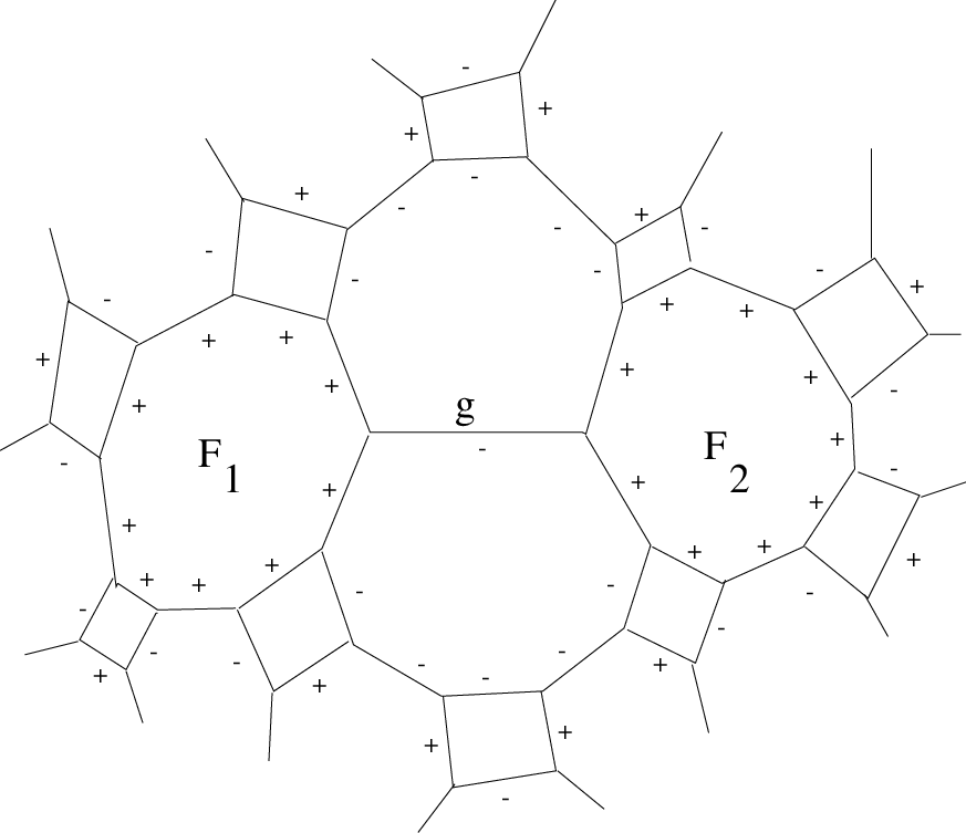
The following is the technical lemma needed above. A proof can be found in the referenced paper.

An easy consequence of this lemma is the following. Let $F_{a},F_{b}$ be two hyperbolic $n$-gons with face angles equal. If we label an $n$-gon $F$ with $+$, $0$ or $-$ by comparing lengths of corresponding sides of $F_{a},F_{b}$, then either $F$ has all sides marked with $0$, in which case $F_{a},F_{b}$ are congruent, or, $F$ has at least four sign changes as we go around the perimeter. This shows that $Q$ satisfies the hypothesis of the theorem.

To show that $F_{1},F_{2}$ are marked $+$ we need to relate the Minkowski inner product to face angles. If two edges of a compact hyperbolic polygon intersect in an angle $\theta<\pi$ then the inner product of their outward normals is $\cos(\theta_{ext})$ where $\theta_{ext}$ is the exterior angle of $\theta$. Now the convex polygons $p_{1},p_{2}$ corresponding to $F_{1}$ in $P^{t}_{\theta_{1}},P^{t}_{\theta_{2}}$ respectively, have the same face angles except at the vertex incident to $g$, where $p_{i}$ has the angle $\theta_{i}$. Thus if the sides of $p_{1}$ where all smaller or equal in length to the sides of $p_{2}$ then we would have by the above lemma that the inner product of the outward normals of the two sides intersecting at $g$ in $p_{1}$ is greater than or equal to the same inner product in $p_{2}$, that is $\cos(\pi-\theta_{1})\geq\cos(\pi-\theta_{2})$. But $\theta_{1}<\theta_{2}$, and therefore the sides of $p_{1}$ must be greater than or equal in length to the corresponding sides in $p_{2}$. This gives the needed step to show that both $F_{1},F_{2}$ are of constant sign $+$.

An ideal hyperbolic quadrilateral has two perpendiculars and it can be shown using elementary hyperbolic geometry that the hyperbolic sine’s of the half lengths of these are reciprocal. The following lemma is a generalization of this fact.

Proof :Choose $\epsilon>0$ such that the one-sided $\epsilon$-neighborhood of $g$ has the same area as $F$.

If we take $N_{\epsilon}$ the two-sided $\epsilon-$neighborhood of $g$ then for each $x\in g$ there is an arc $\gamma_{x}$ perpendicular to $g$ centered at $x$ of radius $\epsilon$. We define three subsets of $g$ as follows:

Therefore $l=l_{0}+l_{1}+l_{2}$ where $l_{i}=$ length of $g_{i},i=0,1,2$.

Each of the sets $g_{i}$ is a collection of intervals. If $A_{1}=$ Area of $F$ outside $N_{\epsilon}$ (cusp region) and $A_{2}=$ area of $F$ consisting of points whose perpendicular geodesic to $g$ has length less than $\epsilon$ (narrow region) then

where $A=A_{1}+A_{2}$ (cusp plus narrow region).

If $e$ is one of the $n-2$ edges of $F$ not intersecting $g$, drop perpendiculars to $g$ from the endpoints of $e$ on $S^{1}_{\infty}$ to the two points $x,y$ on $g$. This forms a quadrilateral $Q_{e}$ with area $\pi$ and base $[x,y]$. Let $A_{e}$ be the area of the region in $Q_{e}$ which is either a distance greater than $\epsilon$ from $g$ or whose perpendicular to $g$ has length less than $\epsilon$. $A_{e}$ is the contribution of $Q_{e}$ to $A$. If $e$ doesn’t intersect $N_{\epsilon}$ then the $A_{e}$ is minimum when $e$ is tangent to $\partial N_{\epsilon}$ (figure 10). If $L$ is the length of the base of the quadrilateral tangent to $\partial N_{\epsilon}$ then

If $e$ intersects $\partial N_{\epsilon}$ at points $x^{\prime},y^{\prime}$ then project down onto $g$ to get points $x_{1},y_{1}$ (figure 11). Now if $\overline{L}$ is the length of either $[x,x_{1}]$ or $[y_{1},y]$ (both have the same length) then

Since we have that $l_{2}\sinh(\epsilon)=l_{0}\sinh(\epsilon)+A$ then

The subset $g_{2}$ consists of at most $(n-3)$ intervals. Therefore by the above, one of these intervals $[a,b]$ must have length $D$ satisfying

Consider the quadrilateral $Q$ formed by taking the two perpendicular arcs $\gamma_{a},\gamma_{b}$ to $g$, centered at $a,b$ respectively, of length $2\epsilon$. Choose the other sides $\alpha,\beta$ to join the endpoints of $\gamma_{a},\gamma_{b}$. There are two edges $e_{3},e_{4}$ of $F$ separated by $g$, which enter and leave $Q$ through the sides $\gamma_{a},\gamma_{b}$. To show that $e_{3},e_{4}$ are close note that they are closer than $\alpha$ and $\beta$ are. The two geodesics $\alpha,\beta$ describe an ideal quadrilateral by extending $\alpha,\beta$ to the sphere at infinity. This quadrilateral has a diagonal of length $D^{\prime}$ which is longer than $D$ whose other diagonal has length $d^{\prime}$. If $d$ is the distance between $e_{3}$ and $e_{4}$ then

Therefore we have

$\blacksquare$

This lemma shows that long geodesics must give thin polygons.

In the hyperbolic plane consider a geodesic $\gamma$ represented by a circle $C$ of radius $R$ intersecting the unit circle at right angles. The two geodesics passing through the origin $o$ meeting $\gamma$ on $S^{1}_{\infty}$ form an angle of $\phi$ at $o$ (visual angle). If $x$ is the Euclidean distance from $o$ to $\gamma$ and $d$ is the hyperbolic distance then we have by simple planar geometry

In $P_{\theta}$ we have planes $F_{1},F_{2}$ intersecting with dihedral angle $\phi$ and let $F_{3},F_{4}$ be the two planes intersecting in edges $e_{3},e_{4}$ respectively of lemma 3. We also have planes $F^{\prime}_{3},F^{\prime}_{4}$ defined by geodesics $\alpha,\beta$ which intersect $F_{1},F_{2}$ at right angles.

If $F^{\prime}_{3},F^{\prime}_{4}$ intersect then $F_{3},F_{4}$ must also intersect. Therefore since planes $F_{3},F_{4}$ cannot intersect then neither can $F^{\prime}_{3},F^{\prime}_{4}$. Looking along the geodesic $g$, $F^{\prime}_{3},F^{\prime}_{4}$ are given by two geodesics $\gamma_{3},\gamma_{4}$ and $F^{\prime}_{3},F^{\prime}_{4}$ by two geodesics passing through the origin and perpendicular to $\gamma_{3},\gamma_{4}$ respectively (figure 12).

Both $\gamma_{3},\gamma_{4}$ have the same visual angle $\phi^{\prime}$. If they are not to intersect then

where $d^{\prime}$ is the length of the short curve on $F$ joining $F^{\prime}_{3},F^{\prime}_{4}$. By lemma 3 we have

Therefore

Therefore we obtain a combinatorial bound on the volume increase by integrating the above equation. This integration is possible as although $\sinh^{-1}(\tan(\phi/2))$ tends to infinity at $\pi$ it is still integrable. Therefore we have

where $K$ is some fixed constant. We can derive this bound in general using the one-parameter family of approximations $X^{t}$ in the same manner as before.

References

- [A] Alexandroff Convex Polyhedra
- [B1] M. Bridgeman Volume increase under Dehn drilling operations Phd. thesis Princeton June 1994
- [B2] M. Bridgeman The Structure and Enumeration of Link Projections To Appear Trans. A.M.S. (1995)
- [Br] R. Brooks On the Deformation Theory of Classical Schottky Groups Duke Mathematical Journal December 1985
- [Th] W. P. Thurston The Geometry and Topology of 3-manifolds
- [HR] Craig Hodgson , Igor Rivin A characterization of Compact Convex Polyhedra in Hyperbolic 3-Space
- [Ho] Craig Hodgson Degeneration & Regeneration of Geometric structures on Three-Manifolds Phd. thesis Princeton June 1986