Tiling a rectangle with the fewest squares.
Abstract
We show that a square-tiling of a rectangle, where and are relatively prime integers, has at least squares. If we construct a square-tiling with less than squares of integer size, for some universal constant .
1 Introduction
A certain store sells square tiles of arbitrary positive integer size for $1 each. You’d like to tile your kitchen (a rectangle, ), for the least cost. What’s the cheapest way?
We show:
Theorem 1
A rectangle, where are relatively prime integers, , requires at least square tiles to tile. Furthermore there exists a square tiling with less than squares of integer size, for some universal constant .
Remark. For the lower bound the sizes of the squares are not restricted to be integers. Also, the quantity in the two bounds is necessary for thin rectangles; for example an rectangle requires at least squares. If is bounded then we have logarithmic upper and lower bounds.
Here for a rectangle we call the aspect ratio the larger of .
In case the aspect ratio of the kitchen is not rational, no tiling with a finite number of squares is possible by a theorem of Dehn [5]; on the other hand, using squares of arbitrary real size, if you have a refrigerator to cover up the untiled portion, you can do equally well:
Theorem 2
For any and , one can tile all but an - neighborhood of a corner of an rectangle with squares, for some universal constant .
Our proof of the lower bound in Theorem 1 uses the theory of electrical networks, which has a well-known connection with square tilings [5, 3, 2]. In particular a generalization of Theorem 1 is as follows:
Theorem 3
Let be a resistor network with underlying graph , with resistances on each edge. If the effective resistance between two vertices is the rational number in lowest terms, then there are at least edges in . Conversely, for any rational there is such a network with a planar graph having at most edges.
Here we allow multiple edges between the same vertices in the graph .
2 The greedy algorithm
Your initial reaction is of course to tile using the greedy algorithm, that is, select the largest square that fits (a tile), place it touching a shortest side of the kitchen, and repeat with the remaining untiled part, which is now .
This method, also known as the Euclidean algorithm, works well for certain shapes of rectangle, for example those rectangles which are , where is the th Fibonacci number. Indeed such a rectangle is tiled with tiles (Figure 1).

Unfortunately for many shapes of rectangles, this algorithm is quite expensive: for a rectangle, the first square leaves a rectangle, which requires at least squares to tile, for a total cost of , which much more expensive than is necessary.
We leave the reader to verify that, if the continued fraction expansion of is , that is,
then the cost of the greedy algorithm on a rectangle is . (Here the integers are called partial quotients of : it is required that and for that . Under these conditions the are uniquely defined except for , and we have assuming .)
For the irrational rectangle , if is the infinite continued fraction expansion of , then the cost to cover up all but the -neighborhood of the corner is
| (1) |
where the is the first number to satisfy
where is the th rational approximant to . Indeed, if the untiled portion after steps is , then we have
or in other words
(Here the depends on the parity of .) If then
Quantities related to this cost for “typical” numbers have been studied in detail. Yuval Peres combined some known results to prove:
Theorem 4 (Peres)
There is a constant such that for any the Lebesgue measure of the set
tends to zero with .
For the proof, see the appendix.
If is irrational and all the are bounded by , then is called -aloof. It is not hard to see (we’ll see later in any case) that if is -aloof, the greedy algorithm gives a logarithmic bound , where the constant depends on .
3 The lower bound.
We give here a proof of the lower bound in Theorem 1. First, the largest square which can fit is a square, which covers of the area, so you need at least squares to tile. We will show that you need at least squares to tile.
To a square tiling of a rectangle , associate a graph as follows [3]: let be the graph with vertex set and edges , where is the set of connected components of the union of the horizontal boundaries of tiles in the square-tiling, and is the set of tiles (note that a tile connects exactly two horizontal components, and that multiple edges between two vertices are possible). The vertex corresponding to the upper boundary of is called , and the vertex corresponding to the lower boundary is . It is clear that is planar, and that and are on the same face (the outer face) of .
It is helpful to direct the edges from the upper vertex to the lower vertex.
Associated to is the resistor network, obtained by assigning each edge of a resistance . By assigning potentials to the vertices and of the network, a flow of electric current is set up in , that is, we have maps (“potentials”) and (“currents”) which satisfy Kirchoff’s rule and Ohm’s law: the net current flow out of any vertex (except and ) is equal to the net flow into that vertex, and the current across an edge equals the drop in potential between its endpoints. (By definition the current has a sign which depends on the direction of the edge.) The potentials and currents are the unique solution to the equations arising from Kirchoff’s and Ohm’s rules with the given boundary conditions . If we denote by the net current going into , then the quantity depends only on the graph and is independent of . This quantity is called the effective resistance, or impedance, from to .
If we scale the square tiling by a homothety of and translate it so that the upper boundary is at -coordinate and the lower boundary is at -coordinate (assuming with loss of generality that ), then we see that a solution (hence the unique solution) of Kirchoff’s and Ohm’s equations is given by: for , equals the -coordinate of the horizontal component corresponding to , and for , is the size of the square tile corresponding to . The quantity is simply the ratio of height to width of the rectangle.
This construction also works in the other direction. We can associate, to any planar graph and choice of two vertices on the same face, a square-tiling of a rectangle whose resistor network is . This is proved in [3], who simply use the idea of the previous paragraph to construct the tiling from the potentials and currents.
By a result of Kirchhoff [8] (see also [3]), the resistance satisfies: , where is the number of spanning trees in , and is the number of spanning trees in , the graph obtained from by gluing together vertices and .
Thus if is a rectangle, we have , and since and are relatively prime, and .
However the number of spanning trees in any graph of edges is less than , since a tree is a subset of edges, and there are distinct subsets of edges. Since has edges, where is the number of tiles, we have . We conclude that .
This gives the lower bound in Theorem 1.
4 The upper bound for real rectangles.
Let be a rectangle with aspect ratio (recall ). We assume : if not, apply the greedy algorithm times. The remaining untiled portion has aspect ratio in the range .
We show how to tile quickly. Assume is .
The idea is simple: use the greedy algorithm, getting a nested decreasing sequence of rectangles (the untiled portions), each containing a fixed corner of , of aspect ratios , with
until some is close to , say for some small . Note then that for we have .
At step , instead of putting in a square, which would result in the new rectangle having aspect ratio , just put in a rectangle of aspect ratio , with its longer side covering the shorter side of . The remaining untiled portion is a rectangle with aspect ratio , and so . Now continue.
Since for each we have , each square added removes either a fraction at least of the area (in the case when one square is added to a rectangle of aspect ratio in ), or a fraction of at least of the remaining area (in case a rectangle of aspect ratio , which is tiled by two squares, is added to a rectangle of aspect ratio ). So the area decreases by a factor of at least
per square added.
This quantity is minimized when , and the rate is .
After squares, the untiled area is a rectangle of area at most , and aspect ratio between and , and so is contained in a neighborhood of radius of the corner.
The completes the proof of Theorem 2.
Remark. The rate of decrease of area is of course not the optimal one. Optimization of similar algorithms seems to be an interesting problem, but one we won’t consider here. One might conjecture that is a lower bound for , since the golden rectangle seems to be most easily tiled by the greedy algorithm, which has this rate.
An alternative method for tiling an rectangle is suggested by the following result of Hall:
Theorem 5 (Hall [7])
Any real number between and can be written as the sum of two -aloof numbers.
Here and are the minimal and maximal possible sums.
So to tile a rectangle, where , write where are -aloof, and divide the rectangle into an and an rectangle with a single vertical line. Now tile each of the subrectangles using the greedy method; by -aloofness, in each subrectangle each new square added takes up at least of the area, so that after squares the remaining area is at most of the original area there. The rate is then .
Our method for integral rectangles will be a variant on this method.
5 An upper bound for rational rectangles.
Let be a rectangle, with , , . We assume as before that : if it is larger, use the greedy algorithm times, so that the remaining rectangle satisfies the above conditions.
We establish in this section an upper bound of for the number of squares needed to tile . Section 7 refines the construction to improve the bound to .
The construction proceeds as follows. Let be -aloof numbers such that (using Theorem 5). Let , and , so that and
We divide the rectangle into a rectangle and a rectangle . We will show (below, after Lemma 8) that we can apply the greedy algorithm successfully to each of these rectangles for a while, that is, until the remaining untiled rectangles each have side lengths for some universal constant (and have aspect ratios ).
We then repeat the process, using Theorem 5 again to subdivide each in two, applying the greedy algorithm until the remainders have sides , and so on.
We show that at each stage the number of squares added in a single rectangle before we subdivide it is at most the logarithm to the base of its larger side length. The side lengths decrease by at least before we resubdivide, and each subdivision doubles the number of rectangles. When the edge lengths of a subrectangle are less than the constant in length, simply tile the subrectangle in any way you please.
We derive for the total number of squares needed to tile:
where is chosen so that that is, , and is the number of squares needed to tile an integer-sided rectangle whose sidelengths are bounded by . (Note that under the map .)
Thus the number of squares is bounded above by
It remains to prove our claim that we can tile a rectangle quickly using the greedy algorithm until the remining untiled rectangle has edges .
Recall that a Farey interval is a subinterval of with rational endpoints which satisfy . (Notationally we allow and .) Each Farey interval gives rise to two Farey subintervals and , and the set of all Farey intervals form a binary tree in this way with the root being . A Farey interval has a label indicating the unique descending path to from the root; this label is a finite word in the letters ‘L’ and ‘R’. thus for example . The Farey interval has the property that for , the continued fraction expansion of begins , and similarly for words ending in . We call a Farey interval finite if .
Lemma 6
If is a finite Farey interval and contains a -aloof number, then .
Proof. If is -aloof, the word such that has no more than consecutive ’s or ’s. In particular , so is in one of the intervals
for which the result is true.
Now if , then clearly , and so each of satisfy the property. If , then and so each of have the desired property. The result easily follows.
Let denote the length of : if then .
Corollary 7
If is a finite Farey interval containing a -aloof number, then .
Proof. If then
The following lemma is the key fact which makes the construction work.
Lemma 8
If is -aloof and then there is a Farey interval containing both and with for some universal constant .
Proof. The Farey intervals nesting down to decrease geometrically in size (with scale at most ) by Corollary 7. So there is a Farey interval containing , with . By backing up at most stages towards the root, there is a Farey interval with such that the distance of to the endpoints of is at least (because in the last 5 letters of there is at least one and one ). Thus contains both and . Furthermore again by Corollary 7. So if , we have
and so taking square roots
and similarly for .
If the word labelling has length , then after adding squares to a rectangle using the greedy algorithm, we find the remaining rectangle is , where
and so
and similarly for .
Now if the aspect ratio or is , then backing up one step gives a rectangle of aspect ratio in and sides bounded by .
This completes the construction.
6 Tiling an “ell”
By an ell we mean a rectilinear polygon (polygon with sides parallel to the axes) with 6 sides. We give here a method for tiling (partially) an ell as in Figure 2

with integer side lengths as indicated, so that the remaining untiled portion is an ell with side lengths of ratios bounded by (i.e. the ratios are all in ). This construction is a subroutine in the algorithm we will devise in the next section.
Let be an ell as in Figure 2. In what follows we describe an ell with four edge lengths : these are the lengths of the four edges corresponding to the edges marked of Figure 2.
Let be given. If either of or (say ) is we add a square of side adjacent to the edge of length , giving a new ell with reduced by ; this does not increase the largest ratio of . So in what follows we assume . By symmetry we may assume either or is the longest edge. There are a number of cases to consider11 1 We apologize for the clumsiness of this algorithm.:
Case 1. Suppose is the longest edge.
Case 1a. Each of the lengths is in the interval . We can assume or else we are done.
Add squares of side length as in Figure 3. The new ell has sides . Each of these is in the interval , since and , and .

Case 1b. All edges are in . Suppose also that .
- •
If , then add a square of side adjacent to edge . This gives a new ell with edges , each in .
- •
If and , add squares as in Figure 4; the remaining ell has edges , and by hypothesis and so each of these is in .

Figure 4: - •
If and then and so .
Case 1c. Edges are in , and .
- •
If , add a square of size adjacent to side . The new ell has sides , each is in ( and ).
- •
If , add squares adjacent to and as in Figure 5; the new ell has edges , each of which is in . (Note .)

Figure 5: - •
If and , add three squares as in Figure 6; the new ell has edges , each of which is in (note ).

Figure 6:
Case 2. Suppose is the longest edge.
Case 2a. Edges are in . Since , we are done.
Case 2b. Edges are in .
- •
If , then and so and we’re done.
- •
If and , then add a square to edge , giving .
- •
If and , then add two squares as in Figure 7, leaving an ell with edges . Note , and so each edge is in .

Figure 7:
Case 2c. Edges are in .
- •
If add three squares as in Figure 3; the ell has edges .
- •
If then , and so .
This completes the construction. Suppose that originally the ratios of were bounded by . Each square added at the first step in this algorithm has side length at least the length of the shortest of . Furthermore, the shortest of never gets any shorter. So each square added takes up at least of the area.
7 A better upper bound for rational rectangles.
We give in this section a refinement of the construction of section 5, yielding a logarithmic bound.
The refinement is based on the following theorem, a two-dimensional version of Theorem 5.
Let be the Cantor set of -aloof numbers.
Theorem 9
For any there is an with the following property. For any positive real numbers with ratios bounded by there exists and such that :
For the proof, see the Section 8.
The correct interpretation of this theorem is as follows: Given the ell of Figure 8, where the sides have lengths in ratios less than , we can find a so that, for the subdivision indicated, the rectangles have aspect ratios in . The quantities of the theorem are the aspect ratios of the as a function of .

Let be a rectangle, , with and again . The construction now proceeds as follows. Let with in Theorem 9. As before, use Theorem 5 to divide into two rectangles , respectively and , with and within of an -aloof number (We assume ).
Apply the greedy algorithm to and as before, until the sides of the untiled rectangles have length , and aspect ratios . (Now the constant here depends on ). It is easy to arrange that and are adjacent, and so the union of the untiled regions then forms an ell.
We claim that we can also arrange so that the ratios of edge lengths of and are at most : simply back up the greedy algorithm if necessary for the smaller of until it is approximately the same size as the other. Since the change in scale between the time the aspect ratio is in and the next time it is in is at most , this proves the claim.
Using the subroutine of section 6, we can tile this ell “easily” (that is, each square added takes up a definite proportion of the area) until all the ratios of sides are less than .
We then apply Theorem 9 with : this subdivides the ell into three rectangles with aspect ratios in . By choosing to be the integer closest to the of the theorem, we can subdivide the ell into three rectangles each with integer sides of length and with aspect ratios within respectively of points in .
We can now use the greedy algorithm on the , until the edge lengths are less than , and the untiled rectangles of respectively, are adjacent, have aspect ratios , and are the same size to within a factor of . (The are not necessarily adjacent to ).
At the next step the ell formed by is tiled using the ell method of section 6 and then is subdivided into “easy” rectangles (using Theorem 9 again), and is subdivided using Theorem 5 into two easy rectangles. As we continue this process, each ell gives rise to an ell and a single rectangle, and each single rectangle gives rise to an ell.
So the total number of untiled rectangles at the th stage of the construction is just the th Fibonacci number: letting be the number of ells and single rectangles, after one iteration we have
As a consequence the number of squares needed to tile is , where:
where as before , is a bound on the number of squares needed to tile a rectangle of edge bounded by , and is a constant depending on . This is a convergent geometric series, since and We have for some universal constant . This completes Theorem 1.
8 Proof of Theorem 9
We will prove a stronger result (Theorem 11).
Recall that a gap of a Cantor set is a connected component of . A Cantor set is called -thick if is obtained from an interval by removing successively open subintervals of which are gaps of , with the property: when an gap is removed from a connected subinterval , leaving intervals on either side with , then and .
Recall that is the Cantor set of -aloof numbers. The following lemma is essentially due to Hall [7] (he studied the case , but his methods extend to any ).
Lemma 10
For any there is an integer such that is -thick.
Theorem 11
Given there exists an with the following property. Let be three -thick Cantor sets in with diameters in ratios bounded by . Let be the orthogonal projection of to along a vector whose coordinates have ratios in absolute value bounded by . Then contains every point in in the convex hull of which is not within a small neighborhood of the boundary of the convex hull of .
Remark. Let us show that this theorem implies Theorem 9. Take to be the Cantor set . For sufficiently large this Cantor set is -thick, by Lemma 10. The set
is a line segment which passes completely through the convex hull of . The direction of is
whose coordinate ratios are bounded in absolute value by by hypothesis (recall ). We need to show that intersects .
Let be the projection given by
(which is not the orthogonal projection, but is orthogonal projection followed by a linear map of bounded distortion). Then is the single point , which is contained in the square because the ratios of any two of are bounded by , and is in turn contained and not close to the boundary of the convex hull of for large (). Thus , and so intersects .
Lemma 12
Fix . If a Cantor set is -thick for some then for some we can remove gaps from the convex hull of , leaving subintervals , with and for each ,
Proof: Since is -thick with , each gap removed from a subinterval leaves two subintervals of length at least th of the length of (since ).
So one simply removes gaps from the convex hull until the remaining subintervals have length between and .
Proof of Theorem 11. Our proof remains at a qualitative level for simplicity. In particular we won’t try to estimate the best .
Let be the convex hulls of . The projection of , the convex hull of , is a hexagon with opposite sides parallel. For such a hexagon H, define to be the set of points in the interior of and at distance more than from any boundary edge of length (see Figure 9). Call the inner neighborhood of .

Define subdivisions of the as in Lemma 12 for some large : so that for we have and . The projection of the union of the convex hulls of the is a “stack” of hexagons as in Figure 10. By Lemma 13 below, is contained in the union of the inner neighborhoods of the “blocks” . Furthermore each block again satisfies the hypotheses of Lemmas 12 and 13, and so we can subdivide it again, and repeat. For each point , we obtain in this way a sequence of blocks converging to . By compactness is contained in .
Lemma 13
Proof. The proof by picture is the most illuminating. The direction of the diagonal edge of the hexagon in Figure 10
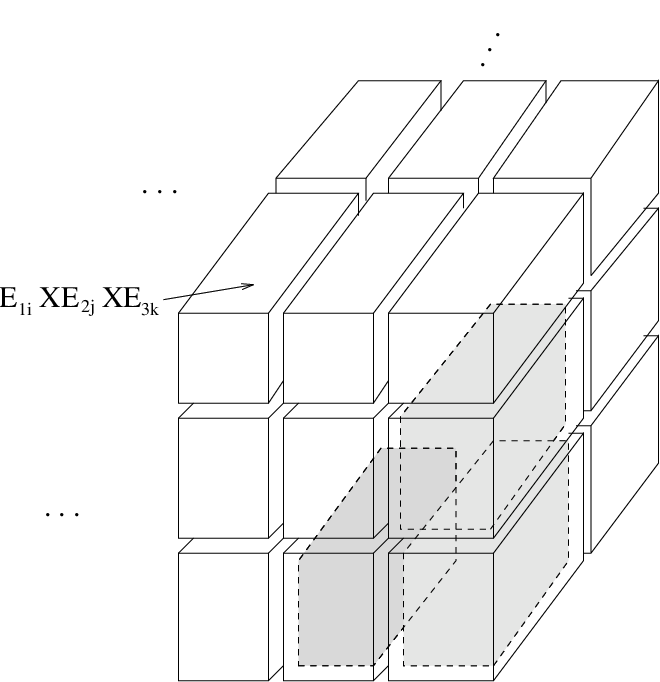
(i.e. the vector ) has slope between and . Using also the fact that the boxes have edge-lengths of ratios bounded by a constant (), their projections are hexagons with edge lengths of ratios bounded by another constant .
Now if , the approximate number of blocks per edge in the stack, is sufficiently large and is sufficiently small compared to the size of the smallest block, we see that the inner neighborhoods of all the boxes cover all of the convex hull of except in a small neighborhood of the boundary; in particular they cover .
9 Problems
Problem 1
What are the best constants in the upper and lower bound of Theorem 1?
Our constructions leave lots of room for improvement in the constant appearing in the upper bound. The lower bound of can also be improved, however. This is another interesting problem in itself:
Problem 2
Among all graphs with edges, which graph has the largest number of spanning trees ? What is the sup of over all graphs? Over planar graphs?
We used the trivial bound for the number of spanning trees of a planar graph. This bound can be improved; N. Young indicated to us an upper bound of for some , which comes from taking into account the vertex degrees.
On the other hand the planar grid graph has converging to (see [4]) as , and this is the largest value we know of. So the actual largest value is somewhere in the range .
Problem 3
How many cubes does it take to tile a box?
None of our methods work for this case; even the greedy algorithm is difficult to define.
10 Appendix
We give here a proof of Theorem 4, which Yuval Peres has kindly allowed us to include.
Recall the notation: and has continued fraction expansion with th approximants .
Let be the sum of the first partial quotients of . Diamond and Vaaler [6] showed that for almost all ,
| (2) |
where (and depends on both and ).
We are interested in . By a result of Khinchin and Levy (cf [1]), for almost every
By discarding a set of measure for any small , this convergence is uniform, i.e. on a set with , we have
We conclude that converges uniformly to on .
Using the Gauss-Kuz’min measure we have for a constant ; and so on we have (using ):
Letting be the complement of this set in , using (2) and we have for all
for some constant .
References
- [1] P. Billingsley, Ergodic Theory and Information. New York: Wiley 1965.
- [2] B. Bollobas, Graph theory: an introductory course. New York: Springer Verlag 1979.
- [3] Brooks, Smith, Stone, Tutte; The dissection of rectangles into squares. Duke Math J. 7, (1940), 312-340.
- [4] R. Burton, R. Pemantle; Local characteristics, entropy and limit theorems for spanning trees and domino tilings via transfer-impedances, preprint.
- [5] M. Dehn; Zerlegung von Rechtecke in Rechtecken, Math. Annalen, 57 (1903) 314-332.
- [6] H. G. Diamond and J. D. Vaaler; Estimates for partial sums of continued fraction partial quotients. Pacific J. Math. 122 (1986):73-82.
- [7] M. Hall; On the sum and product of continued fractions. Annals of Math, 48 (1947):966-993.
- [8] G. Kirchhoff; Über die Auflösung der Gleichungen, auf welche man bei der Untersuchung der linearen Verteilen galvanisher Ströme geführt wird, Ann. Phys. Chem. 72 (1847):497-508.