Spaces of locally convex curves in
and combinatorics of the group
Nicolau C. Saldanha and Boris Shapiro
Dedicated to the memory of the one and only
Vladimir Igorevich Arnold
Abstract.
In the 1920’s Marston Morse developed what is now known as Morse theory
trying to study the topology of the space of closed curves
on ([7], [5]).
We propose to attack a very similar problem,
which 80 years later remains open,
about the topology of the space of closed curves on
which are locally convex (i.e., without inflection points).
One of the main difficulties is
the absence of the covering homotopy principle for the map sending a
non-closed locally convex curve to the Frenet frame at its endpoint.
In the present paper we study the spaces of locally
convex curves in with a given initial and final Frenet frames.
Using combinatorics of ,
where is the usual Coxeter-Weyl group,
we show that for any these spaces fall in at most
equivalence classes up to homeomorphism.
We also study this classification in the double cover .
For our results complete the classification
of the corresponding spaces into two topologically distinct classes,
or three classes in the spin case.
In what follows we will study different spaces of curves
(or to );
we start with some basic definitions.
A smooth curve is called locally convex
if its Wronskian
is non-vanishing for all
(see [1], [11], [12], [13]).
A smooth curve is called (globally) convex
if for any linear hyperplane
the intersection consists of at most
points counting multiplicities;
it is an easy exercise to check that global convexity implies local.
Observe that if is locally convex
then so is its spherical projection
.
Notice that for , a curve
is locally convex if its geodesic curvature is never zero
(and therefore has constant sign) and a closed curve
is globally convex if it is the boundary of the intersection
of the sphere with a convex cone.
For various technical reasons,
the space of smooth curves is too small and not the most adequate.
The definition of local convexity makes sense for other spaces,
such as the Banach spaces ,
and the Sobolev spaces , .
In Section 2 below we shall introduce an “official” topology
for the spaces of locally convex curves:
this turns out to be a Hilbert space containing
all the above spaces.
As with other questions concerning infinite dimensional topology,
the choice of space actually has little consequence.
Locally convex curves in are closely related
to fundamental solutions of linear
ordinary homogeneous differential equations of order
on with real-valued coefficients.
Namely,
if are linearly independent solutions
of an equation
with , ,
then is locally convex.
A locally convex is called positive if
and negative otherwise.
From now on we mostly consider positive curves.
Given a smooth positive locally convex ,
define its Frenet frame
as the result of the Gram-Schmidt orthogonalization
of its Wronski curve
.
In other words, satisfies the relation
where is an upper triangular matrix
with positive diagonal.
Let be the space of all positive locally convex curves
(in the appropriate space, to be defined in Section 2)
with the standard initial frame ,
where is the identity matrix of size .
As we shall see (Lemma 2.3),
the space is a contractible Hilbert manifold
and therefore diffeomorphic to Hilbert space.
Given , let
be the set of positive locally convex curves on with the
standard initial and the prescribed final frame ;
one of the main difficulties is that the map
taking to is not a fibre bundle.
Let ()
be the universal cover (recall that this cover is a double cover).
Denote by the identity element
and by
the unique nontrivial element with .
For , the map
can be uniquely lifted to ,
, .
Given , let
be the set of positive locally convex curves
with .
One can immediately observe that
.
The Hilbert manifolds and for various
and
are the main objects of study in this paper.
Some information about the topology of ,
mostly in the case or in the case ,
was earlier obtained in [1], [6],
[8], [9], [11],
[12] and [13].
In particular, it was shown that the number of connected components of
equals for even
and for odd , which is related to the existence of closed globally convex
curves on all even-dimensional spheres.
It was also shown in [1]
that for even the space of closed globally convex curves with a fixed
initial frame is contractible.
The first nontrivial information about the
higher homology and homotopy groups of these components
can be found in [8] and [9].
In this paper we leave aside the fascinating and widely open question
about the topology of the spaces and
concentrate on the following.
Problem 1.
How many different (i.e., non-homeomorphic) spaces
are there among , , ?
Analogously, how many different spaces are there among
, ?
To formulate our partial answer to the latter question
we need to introduce the following set of matrices.
For a positive integer let
be the diagonal matrix whose
first entries equal to and the remaining
entries equal to .
Notice that equals both the trace and the signature of
and that if and only if .
In the latter case, let
be the two preimages of .
Our first result is as follows.
Theorem 1.
For , any ,
and any one has:
(1)
Each space is homeomorphic to one of the subspaces
, where ,
(there are such subspaces).
(2)
For even, each space , ,
is homeomorphic to one of the subspaces ,
,
,
, …,
,
.
(3)
For odd, each space , ,
is homeomorphic to one of the subspaces
, ,
,
, …,
,
, .
Using Theorem 2 below and results proved elsewhere
([8], [9]) we check that for
the above spaces are pairwise non-homeomorphic.
It is natural to ask whether
they are likewise non-homeomorphic for ;
see discussions in the first subsection of the conclusion.
We might want to describe the topology of these spaces;
the next result gives some partial answers.
Let (resp. )
be the space of all continuous curves
(resp. )
with and
(resp. and ).
Using the Frenet frame we define Frenet frame injections:
It is a classical fact that the value of (resp. )
does not change the space
(resp. ) up to homeomorphism.
Therefore, we usually omit (resp. ) and write
(resp. ) instead.
Theorem 2.
For , consider the Frenet frame injections as above.
(1)
For all and for all
the maps and
are weakly homotopically surjective.
(2)
If then the Frenet frame injections
and
are weak homotopy equivalences.
In this case there exist homeomorphisms
Recall that a map is weakly homotopically surjective
if the induced maps are surjective;
also, a map is a weak homotopy equivalence
if the induced maps are isomorphisms.
Notice that, in general,
for arbitrary or it is by no means true
that the Frenet frame injection induces a homotopy equivalence:
even the number of connected components can be different.
Versions of Theorems 1 and 2
also hold for the spaces and
.
These facts follow from our results
together with Theorem 2 in [4];
alternatively, our proofs can be adapted
(with some extra rather routine work).
Acknowledgements.
The first named author gratefully acknowledges the support
of CNPq, FAPERJ and CAPES (Brazil) and is sincerely grateful to
the mathematics department of the Stockholm University for
the kind hospitality during his visits to Sweden in 2005 and 2007.
2. Frenet frames and Jacobian curves
We collect in this section a few basic notions and facts.
The logarithmic derivative of a curve
is defined as .
Notice that
belongs to the Lie algebra and is therefore
automatically skew symmetric.
Let be the set of
tridiagonal skew symmetric matrices
with positive subdiagonal entries,
or skew Jacobi matrices, i.e.,
of matrices of the form
A curve is called Jacobian
if its logarithmic derivative satisfies
for all
(where is an interval).
Lemma 2.1.
Let be a smooth curve with .
The curve is Jacobian if and only if
there exists with .
Recall that a smooth curve
belongs to if and only if
and is (positive) locally convex:
Proof.
Consider and its Wronski curve
We have
for an upper Hessenberg matrix whose subdiagonal entries equal to :
Recall that is upper Hessenberg if whenever .
Write and substitute for
in the equations above to obtain
and therefore
which is upper Hessenberg with positive subdiagonal entries
(the first product is upper triangular,
the second one is upper Hessenberg).
Since we know that ,
we have , proving one implication.
For the other implication, consider
such that ,
and for all .
Set .
We have ,
.
Similarly,
where and the values of are not important.
In general
Thus applying Gram-Schmidt to the Wronski curve
yields ,
completing the proof.
A smooth Jacobian curve is called
globally Jacobian if ,
, is globally convex.
Notice that given a smooth function
the initial value problem
yields as in the lemma and therefore
a smooth curve .
This establishes a homeomorphism between the space
of smooth curves
and the convex set of smooth functions .
We will denote this correspondence by
It will be convenient to have examples of locally convex curves
and corresponding Jacobian curves.
Lemma 2.2.
For let
and () be positive parameters with
mutually distinct and . Set
For let
, and () be positive parameters with
mutually distinct and . Set
In both cases the curve is locally convex
with constant .
Conversely, if is locally convex
with constant then
for some and as above
(for appropriate and ).
Furthermore,
assume and set
and : we have .
For , is a circle;
for , turns around in one plane
while it turns around at a faster rate in another plane:
for suitable values of and , looks
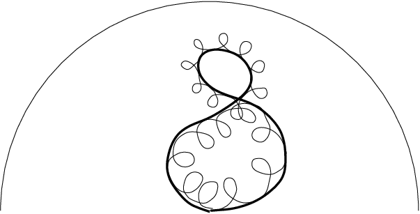
like a phone wire (see Figure 1).
Figure 1. A phone wire is locally convex in
Proof.
A straight-forward calculation gives,
for ,
and for ,
Alternatively, we can compute
and its logarithmic derivative :
it turns out to be a constant element of .
In general, if and is locally convex
then so is : thus, is locally convex.
Conversely, assume
and that is constant equal to ;
we then have .
The eigenvalues of are all on the imaginary axis
and therefore of the form , ,
plus a in case is odd.
Thus there exists such that
Write
Thus, according to parity we have:
and therefore
Up to multiplication by a matrix of the form
,
can be assumed to be of the form
for
(with a corresponding change of ).
The formulas in the previous paragraph of this proof
indicate that the parameters
and must be positive and that the ’s must be pairwise distinct
for to be locally convex, as desired.
The other claims are easy.
The space of smooth curves is not the most convenient, however;
we use the above correspondence to define our favorite space of curves:
if we consider
we can solve the initial value problem and determine
and .
Notice that the curve constructed in this way from
belongs to
but the concept of local convexity does not make sense
for all curves
with .
A minor inconvenience is that is not a Hilbert manifold;
we resolve this problem by defining a diffeomorphism
with -th coordinate
, .
Given we set
and as above,
thus defining a space of Jacobian curves
and an explicit diffeomorphism .
There are sometimes advantages in working with
rather than : for instance, multiplication
(in ) allows for a sort of superposition.
This will be useful later in the paper.
Given let
be the space
of Jacobian curves
with , .
Finally, we use the map to define the spaces
and , which are now Hilbert manifolds.
Recall also that two Hilbert manifolds are diffeomorphic
if and only if they are homeomorphic which, in its turn, holds
if and only if they are weakly homotopically equivalent ([3]).
Besides the Hilbert manifold structure,
the above definition of the spaces (and other spaces)
has the advantage
of allowing discontinuities in
thus bypassing the need for a roundabout smoothening process.
The following result is now trivial.
Lemma 2.3.
The space is contractible.
3. Bruhat cells and the Coxeter-Weyl group
As a first step, for any fixed dimension
we reduce Problem 1
to consideration of only finitely many different
values of and using well-known group actions.
The key observation here is that if
is positive locally convex and has positive
determinant then both
and
with
are positive locally convex.
Let be the group of real upper-triangular
matrices with positive diagonal
and
be the subgroup of matrices with diagonal entries equal to one.
Consider the action of on
by conjugation:
in what follows we will refer to the action
of on different spaces as the Bruhat action.
This action induces the action of on
as the postcomposition of the conjugation
with the orthogonalization.
In other words,
where is the only matrix in
such that ;
thus, is obtained from by Gram-Schmidt.
It is well-known that the Bruhat action on
has finitely many orbits.
These orbits are referred to as the Bruhat cells of :
two orthogonal matrices belong to the same
Bruhat cell if and only if there exist
upper triangular matrices , with positive
diagonal satisfying .
We denote the Bruhat cell of by
.
Let be the Coxeter-Weyl group
of signed permutation matrices and let
.
Let be
the subgroup of diagonal matrices with entries and determinant ;
thus is isomorphic to .
Each Bruhat cell contains exactly one element
and is diffeomorphic to a cell
whose dimension equals the number of inversions of .
In other words, for each
there is a unique
such that there exist satisfying .
We recall an algorithm producing from a given ;
this algorithm will be used later,
particularly in the study of chopping.
Consider the first column of and look for the lowest non-zero entry,
say .
We first multiply by a diagonal matrix
to obtain a new matrix for which ;
for simplicity, we may thus assume .
We next perform row operations on to clean the first column above row :
in other words, we obtain such that
satisfies ;
again assume from now on that .
Now perform column operations on to clean row
to the right of the first column, i.e.,
obtain such that
satisfies .
Repeat the process for each column:
at the end of the process we obtain
()
for which there exists a permutation such that
.
In other words, ;
since
we have and .
Recall that
is a group homomorphism and the double cover of
(for , this is the universal cover).
Let
the groups and
are -central extensions of and ,
respectively.
Notice that
for instance, is isomorphic to
the quaternion group .
The Bruhat cell decomposition can be lifted to
where each cell contains a unique element of .
Two elements of or
will be called Bruhat equivalent
if they belong to the same cell
in the corresponding Bruhat decomposition.
We will also write
for the Bruhat cell of .
The Bruhat action of on induces the Bruhat action
of on the space as follows:
given and ,
set
(where ).
Clearly, if
then .
The following lemma is now easy.
Lemma 3.1.
If (resp. )
are Bruhat equivalent then and
(resp. and ) are homeomorphic.
This explicit homeomorphism will be used again
and we therefore introduce some notation.
Let and be as in the lemma:
there exists a matrix
with and therefore .
Define
by
(for ).
Similarly define .
Proof.
The map is a homeomorphism
with inverse ; the spin case is similar.
4. Time reversal
In this and the two following sections
we introduce three natural operations
acting on and on the spaces of curves under consideration.
The naive idea here would be to consider the curve
;
this curve however may be negative locally convex
and has the wrong endpoints:
we show how to fix these minor problems.
Let ;
notice that .
For , define .
The map is an anti-automorphism
which lifts to an anti-automorphism .
Indeed, given consider a path
with , ;
let and
with ;
lift to define
with ; define .
The map is well defined:
two homotopic paths and
yield homotopic paths and ;
the paths and are also homotopic
(apply to the homotopy) and therefore
.
These two anti-automorphisms
preserve the subgroups
and .
In fact, the map
admits a simple combinatorial description:
the matrix is obtained from
by transposition and the change of sign of
all entries with odd.
We do not present a detailed combinatorial description of
in but we record an observation for later use.
Lemma 4.1.
Let , , .
Then there exists
with and .
Proof.
Let
and with . We claim that satisfies the claim;
in order to perform this computation we construct paths in
and lift them to .
Write
Take
with small blocks,
one large block followed by ones.
Now lift the path to
with :
without loss of generality, .
Clearly and
Thus and are only different in two
of the coordinates of the block, where one makes a half-turn
one way and the other makes a half-turn the other way.
Thus , as required.
Notice that the map
given by
satisfies for .
For ,
define its time reversal by
where is the transpose of .
Lemma 4.2.
For any we have
.
Furthermore,
In particular, if is a locally convex curve
for which is constant then .
Time reversal yields explicit homeomorphisms
Proof.
Consider a smooth curve ;
we must check that is positive locally convex:
we have
and therefore
We must now check that and
.
Recall that
where and are upper triangular matrices
with positive diagonal.
We have
and therefore
Since
and
is upper triangular with positive diagonal
we have
in particular,
This completes the proof of the first claim
and of the first identity for smooth ;
the second identity follows by taking derivatives
and the final claim is now easy.
The identities are extended to the general case
(i.e., not necessarily smooth) by continuity,
thus completing the proof.
5. Arnold duality
Let
be the anti-diagonal matrix with entries
;
for instance, for and we have, respectively,
this matrix will appear in several places below.
Define an automorphism of by ;
notice that the subgroup
is invariant under this automorphism.
As before, lift this automorphism to define an automorphism
(also called ) of and .
The combinatorial description of on is the following:
rotate by a half-turn
(meaning that the -th entry of
becomes the -th entry of the new matrix)
and change signs of all entries with odd.
Notice that the map
given by takes to itself (as a set),
but reverts the order of the subdiagonal entries.
For , define its Arnold dual as
It turns out that this operation is just the usual projective duality
between oriented hyperplanes and unit vectors in disguise
(comp [2]).
Lemma 5.1.
For any one has
that .
Furthermore,
Arnold duality gives explicit homeomorphisms
Proof.
We must first check that if is smooth
then as defined above also belongs to .
Consider given by
We have
by Lemma 2.1,
for :
thus ,
completing our first check.
The formulas for and
have also been proved for smooth and therefore,
by continuity, for all .
The formulas imply that
if then .
The final claim is now easy.
6. Chopping operation
The first two operations corresponded to -symmetries
in ;
our third operation is quite different,
loosely corresponding to taking
and chopping off a small tip at the end.
We again start with algebra and combinatorics.
For a signed permutation
and a pair of indices with
define to be the number of pairs with
, and .
In other words, is
the number of nonzero entries of in the northeast quadrant.
Also set
It is easy to check that for all one has .
Using the above notation define
where is the only index for which .
Additionally, define
Lemma 6.1.
.
Proof.
Indeed, let be the permutation such that
if is the only index for which .
Then
Thus is a function from
to .
Notice that for any .
We extend to a function from to
by declaring that if and are Bruhat equivalent
then ; we similarly extend the function to .
The map is a projection
(in the sense that )
and therefore defines a partition of
into classes of the form , .
Furthermore, if ,
we have so that
a class is a fundamental domain
for the action of on by multiplication.
Let be the matrix used in the definition of Arnold duality.
Notice that
and therefore for all .
For , its chopping is defined by .
Thus the Bruhat equivalence class of is an open set,
dense in .
The maps and
as well as the functon
will play a crucial role in our argument.
(Notice that is not a group homomorphism).
Let us present a geometric interpretation for and .
For and ,
we define the naive chop of by as
A straightforward computation gives
in particular,
The inconvenience here is that if is fixed
and varies over the whole
we have no control of ,
the final frame of .
The situation improves if we adapt the choice of
depending on and focus on Bruhat cells
instead of individual final frames.
Lemma 6.2.
For any and for any
there exists such that
for all
we have that .
In other words, given
there exists such that,
for all ,
is Bruhat equivalent
to .
Before proving Lemma 6.2 we present
an illustrative example for .
Take
and expand an arbitrary smooth curve
in a Taylor series near . Using
we get
(up to higher order terms) so that,
for ,
We now apply the above algorithm
to find which is Bruhat equivalent
to when is a negative number with a small absolute value
(i.e., ).
We start at the -th entry , which is positive.
Thus, .
We now concentrate on the (i.e., bottom left) -blocks
of and :
since ,
the signs of the determinants of these two blocks should be equal;
since its original value equals ,
the -th entry of equals .
Finally, the -th entry must be set to
for the whole determinant to be positive.
Summing up, if
then there exists
such that for any
one has that is Bruhat equivalent to
The general proof below follows the same idea.
Proof.
As above, consider
with associated permutation ,
so that if and only if .
Write a Taylor approximation
where
where
Let be the -block of :
from the algorithm, we must show that, for small negative ,
the matrix is invertible and compute the sign of its determinant.
Write for
Here we use the notation .
Let be the -blocks
of , respectively.
Similarly, let and be the
and -blocks
of and , respectively.
We have
and therefore is the product of the determinants
of these blocks. We must therefore determine the sign of the determinant
of each block.
For real numbers and , we write
if and have the same sign.
We have ,
,
and .
In order to compute , consider the Vandermonde matrix
with ;
notice that there exists with .
Let be the -block of ,
also a Vandermonde matrix. We have
At this point we know that
(with the same sign for all small negative )
and therefore there exists a diagonal matrix
such that and are Bruhat equivalent.
Write ;
we must compute .
Let be the -block of :
by Bruhat equivalence we have ;
by construction we have
.
Thus .
We have
and therefore
Since both sides have absolute value the latter relation is actually an equality;
for and we then have
Thus and we are done.
A geometric description of the situation is now more clear.
The Bruhat cells of the form , ,
are disjoint open sets and their union is dense in .
The complement of this union is the disjoint union
of Bruhat cells of lower dimension.
Let be a smooth Jacobian curve
(i.e., with
for all ):
if does not belong to a top-dimensional Bruhat cell
then the function and Lemma 6.2
tell us in which cell falls for , small.
In other words, provided you follow a Jacobian curve you can only arrive at a given low-dimensional
Bruhat cell from one of the adjacent top-dimensional cells.
As discussed above, the decomposition into Bruhat cells
lifts of .
The above geometric characterization of
thus also lifts to a map
.
Let (so that )
and define
by .
We shall not attempt to give a combinatorial description
of or in the spin groups.
We present yet another interpretation of the chopping operation.
Let
be a Jacobian curve.
Notice that if is Jacobian and
then so is (their logarithmic derivatives are equal).
Thus, Lemma 6.2 can be extended to show
that for all one has that
or
.
In particular, taking , we have
.
Conversely, given and
there exists
a globally Jacobian curve
with ,
(so that , ,
is globally convex).
The following statement thus follows from Lemma 6.2.
Corollary 6.3.
Given there exists an open set
with and .
Similarly, given
there exists an open set
with and .
Proof.
The case follows from the remarks above
together with Lemma 6.2;
the case is similar.
The next statement is crucial in our consideration.
Proposition 6.4.
For any
there are homeomorphisms
We need a few preliminary constructions and results.
Consider a Jacobian curve
with and . Define
by
Lemma 6.5.
Consider a globally Jacobian curve
whose image is contained in a Bruhat cell.
Let , and
with .
Then the maps and
are homotopic. In particular,
is a homotopy equivalence.
Proof.
Since and
are in the same Bruhat cell for all we can define
a continuous function
with , , .
Define
by
The map produces the desired homotopy from
to .
To prove Proposition 6.4
we will also use the following previously known facts.
For any the space
has two connected components if and only if
there exists a globally convex curve in .
One of these connected components
is the set of all globally convex curves in
and this connected component is contractible.
If contains no globally convex curves
then it is connected.
Let and be two topological Hilbert manifolds. Then
any weak homotopy equivalence is homotopic
to a homeomorphism .
Let and
consider a smooth Jacobian curve
with .
Choose sufficiently small so that the image of
.
Let ,
.
Proposition 6.4 now follows
directly from the next lemma.
Lemma 6.6.
The map
is a weak homotopy equivalence.
Proof.
For a non-negative integer,
let :
we construct
and a homotopy
with , .
By compactness and continuity, there exists such that
for all and for all
we have .
Again by compactness and continuity, there exists ,
, such that for all
we have .
Thus, for each ,
the space of globally Jacobian curves
for which and
is non-empty
(since ) and therefore,
by Fact 1, a contractible space.
Consider the subspace of curves
for which for ;
the condition
implies that is non-empty and Fact 1
implies that is also contractible.
We may therefore construct
a homotopy
with ,
and .
In other words, we may assume without loss of generality
that there exists such that
for all and .
Set and
with .
We may reparameterize the curves so that, for all ,
and for .
In other words, we may assume that
.
Set ;
Lemma 6.5 tells us that
is a homotopy equivalence:
is therefore homotopic to
for some ,
implying that is homotopic to
, as desired.
This completes the proof that
is surjective.
The proof that this map is injective is similar.
Let and
;
assume that is homotopically trivial,
i.e., that there exists
with :
we need to prove that is homotopically trivial.
As above, change so that agrees with
near , i.e., we may assume to be of the form
.
We therefore have that
is homotopically trivial.
Since
is a homotopy equivalence we are done.
First we reformulate Theorem 1
using the language of the prevous sections.
Theorem 3.
Let : if then
and are homeomorphic.
Let : if and
then
and are homeomorphic.
Theorem 1 follows directly from Theorem 3.
The condition in the spin part is necessary:
for and the two central elements
the spaces and are not homeomorphic
since they have different numbers of connected components.
Recall that from Lemmas 3.1 and 6.6
and Proposition 6.4
we already know that if
then and
(as well as ) are homeomorphic;
we have a similar result for the spin group.
We are therefore left to consider the spaces ,
, and their spin counterparts.
A number of additional statements are required for
the proof of Theorem 3.
Lemma 7.1.
Let with .
Then there exists with
, .
Thus and are homeomorphic.
Proof:
Let be a permutation of
with for all .
Let be a permutation matrix with
if and only if .
Set :
we have .
On the other hand, if ,
we have
(from the proof of Lemma 7.3)
and therefore
and .
The last claim follows from Proposition 6.4.
This completes the proof of Theorem 3
for the case:
one judicious use of the equivalences
proved in the previous section is enough.
The spin case is slightly subtler:
it turns out that a single instance of the equivalences
is not enough, which can be readily checked
by an exhaustive search in the case .
A small chain of consecutive instances of the equivalences are
therefore used.
Lemma 7.2.
Let
with .
Then there exist with
,
and either
or .
Thus and are homeomorphic.
Proof.
Take and apply Lemma 4.1
to obtain
with .
Let , , .
By Lemma 7.1 there exist
with , ,
, .
Take with
, ,
, .
We have and and
we are done.
Theorem 3 follows directly from
Lemmas 7.1 and 7.2.
It is natural to ask whether Theorem 3 is the strongest
possible such statement, i.e., if spaces which it does not declare
homeomorphic are actually not homeomorphic.
We do not know the answer to this question
(see Problem 2 below)
but the following proposition shows that it is the strongest
result which follows (or follows directly)
from the remarks of the previous sections.
Our nearest goal is to prove Theorem 2(i),
i.e. the fact that the inclusion
is homotopically surjective
for all and then to settle Theorem 2(ii),
i.e. that this inclusion is a homotopy equivalence if .
Recall that the group
has a natural Riemann metric and inherits it via .
With this metric,
let be the injectivity radius of the exponential map,
i.e., is such that if ,
, then there exists a unique shortest
geodesic
(parametrized by a constant multiple of arc length)
joining and so that , .
We will need another technical lemma.
Lemma 8.1.
Let be a smooth compact manifold and
be a smooth function
and write .
Then there exists
and corresponding such that
and
the curves
are positive locally convex for all .
Furthermore, given , ,
we may assume that
for all , .
The intuitive picture here, at least for ,
is that an arbitrary curve
can be replaced by a phone wire,
a locally convex curve which in some sense follows
while quickly rotating in a transversal direction to guarantee local convexity
(see Figure 2).
Figure 2. Approximating a curve by a locally convex curve
Proof:
Take as in Lemma 2.2.
We claim that
satisfies the lemma for a sufficiently large integer .
Notice that
and
where tends to when .
Since
is positive and bounded away from it follows that
is indeed locally convex for sufficiently large .
Furthermore, the identities
where and
are upper triangular matrices with positive diagonals,
show that
can be made arbitrarily small by choosing large .
Proposition 8.2.
For any
the inclusion
is homotopically surjective.
In other words, given
there exists a homotopy in from to
.
Proof.
Write .
Assume without loss of generality that is smooth
if interpreted as .
We may also assume that is flat at both and , i.e.,
that for ,
for all and all .
By Lemma 8.1,
there exist
and corresponding
such that
for all , ;
here, as in Lemma 8.1,
.
The flatness condition guarantees that
Recall that :
let be a homotopy
between the constant path and .
Take and
.
Clearly,
,
as required. It suffices to construct homotopies between
and and between and .
The homotopy between and is given by
Recall that :
the homotopy between and
is defined by joining these two points of
by the uniquely defined shortest geodesic
(parametrized by a constant multiple of arc length):
Proposition 8.3.
Assume :
then the inclusion
is a weak homotopy equivalence.
In other words (given Proposition 8.2),
if
takes
to
then there exist
and corresponding
with
.
Clearly if then must be , or .
Theorem 2 therefore follows
from Proposition 8.3 and Fact 2.
Proof.
Assume without loss of generality that is smooth.
Take as in Lemma 8.1
so that, for any ,
.
We may furthermore assume that the curves
are locally convex for any ,
for any and for any .
Recall that for some large :
take to be a multiple of so that
,
and .
Recall that is constant:
let .
Set
We now define in the two regions
and .
For we squeeze the function
to a central interval and attach chunks of
outside the central interval.
For
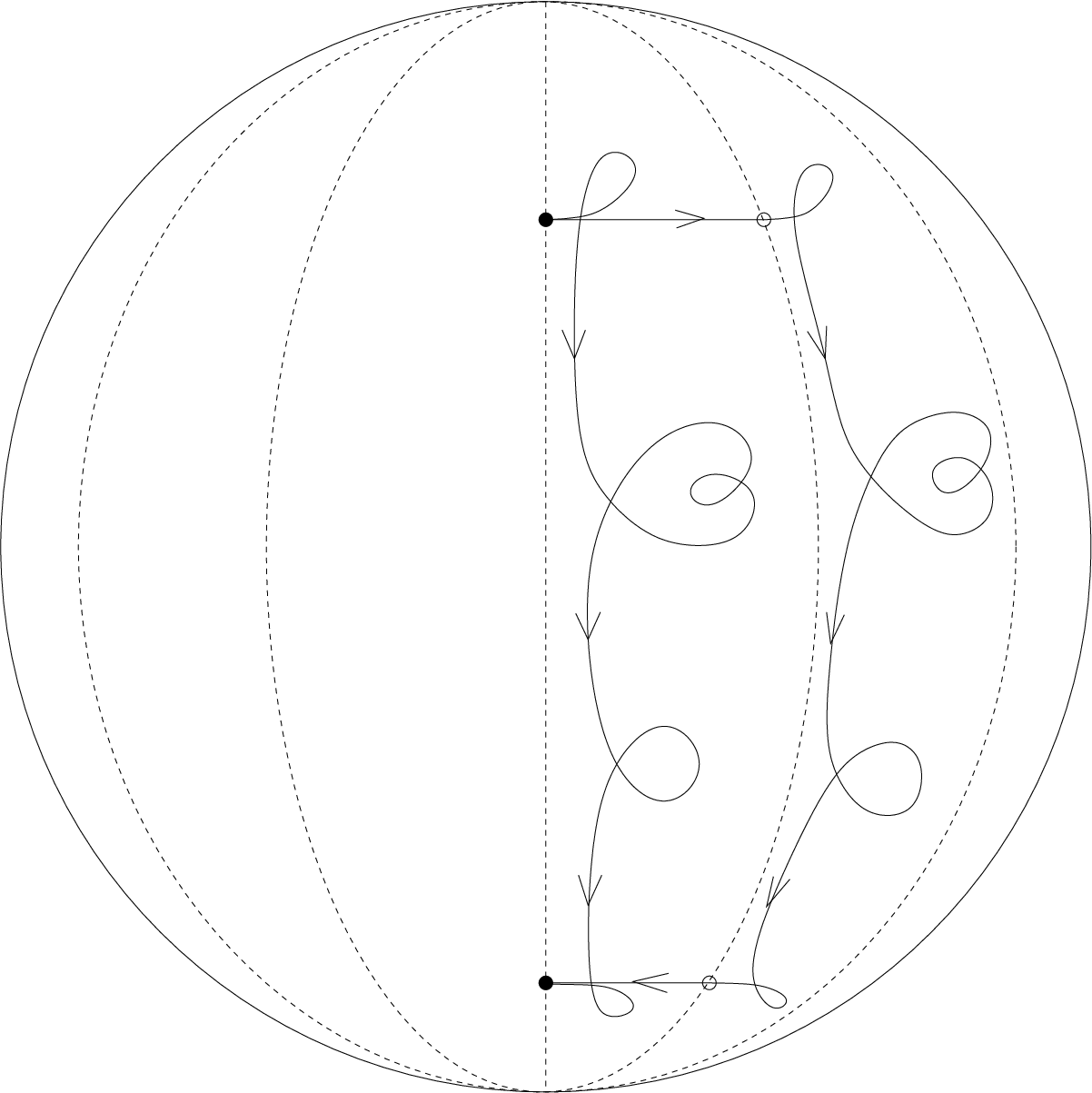
the construction is illustrated in
Figure 3:
we can add chunks of a locally convex curve at the endpoints
and translate in the sphere (i.e., rotate in )
the central portion of the curve.
Continue the process to add several closed circles
at both endpoints.
Figure 3. Approximating a curve by a locally convex curve
The general construction is perhaps best stated
in terms of : for
Recall that is only assumed to be of class
and therefore the jump discontinuities are allowed.
The curve defined using the above
is by construction locally convex:
we must verify that .
We have ;
for we therefore have
and ;
finally, at least in we have
(recall that and that
);
by continuity we have in
for all with .
The missing step is .
For , the circles which are concentrated at the endpoints
for must spread along the curve as approaches .
More algebraically, notice that
for both and , we can write
,
, .
From the constructions above we have
We are left with proving that is locally convex.
For ,
is a reparametrization of and therefore locally convex.
For ,
locally convexity follows from Lemma 8.1 or,
perhaps more precisely, from the choice of
as described at the beginning of the proof.
Finally, for ,
is a reparametrization of
and therefore again locally convex.
This completes the construction of and the proof.
For , Theorems 1 and 2 imply
that any space is homeomorphic to one of three spaces
,
or .
From [6], we know that and
have and connected components, respectively,
and is clearly connected.
From [8] and [9], we know that
,
and .
Thus, these three spaces are not pairwise homeomorphic;
also, the non-contractible connected component of
is not homeomorphic to
either or .
Unfortunately, similar information is unavailable for .
We formulate the following question.
Problem 2.
Are the subspaces
(and similar space of curves in )
appearing in Theorem 1
pairwise non-homeomorphic for ?
Our best guess is that the answer is positive.
9.2. Bounded curvature
A first natural generalization of the space of locally curves on
is the space of curves whose curvature at each point is
bounded by two constants .
Problem 3.
Is it true that there are only
finitely many topologically distinct spaces of curves whose curvature is
bounded as above among the spaces of such curves with the fixed initial and
variable finite frames?
9.3. Other Lie groups
The space is a special instance
of a more general construction on an arbitrary compact Lie group.
Given a compact Lie group , consider a non-holonomic subspace
of its Lie algebra (i.e., this subspace generates the whole algebra).
Consider some polytopal convex cone in this subspace.
Take the left-invariant distribution of cones on obtained
by its left translation in the algebra.
Finally, consider spaces of curves on tangent to the
obtained cone distribution which start at the unit element and end at some
fixed point of .
This generalization includes the scenario described in the previous
subsection as a special case ( is and the subspace consists
of skew tridiagonal matrices, just as for our problem;
the only difference is the cone).
Problem 4.
Is it true that there are only
finitely many topologically distinct spaces of such curves with the fixed
initial and variable finite point?
This is likely to be too optimistic an attempt of generalization,
but perhaps the finiteness condition holds true
with some interesting additional hypothesis.
For instance, our cone is the interior of the convex hull of a small
set of rather special vectors: maybe some such condition is needed.
9.4. The homotopy type of spaces of closed locally convex curves
Finally, the most interesting problem in this context
is to describe the homotopy type of the space of closed locally convex curves.
The aim of [10] is to address this problem for ;
see partial results in [8], [9].
References
[1]S. Anisov,
Convex curves in .
Proc. Steklov Inst. Math, 221:2 (1998), 3–39.
[2] V. I. Arnol’d,
The geometry of spherical curves and the algebra of quaternions,
Russian Math. Surveys 50:1 (1995), 1–68.
[3]D. Burghelea, D. Henderson,
Smoothings and homeomorphisms for Hilbert manifolds,
Bull. Am. Math. Soc. 76 (1970), 1261–1265.
[4]D. Burghelea, N. Saldanha, C. Tomei,
Results on infinite dimensional topology and
applications to the structure of the critical set
of nonlinear Sturm-Liouville operators,
J. Differential Equations 188 (2003), 569–590.
[5] W. Klingenberg,
Lectures on closed geodesics.
Grundlehren der Mathematischen Wissenschaften, Vol. 230.
Springer-Verlag, Berlin-New York, 1978, x+227 pp.
[6]J. A. Little,
Nondegenerate homotopies of curves on the unit 2-sphere,
J. Differential Geometry, 4 (1970), 339–348.
[7] M. Morse,
The calculus of variations in the large.
Reprint of the 1932 original.
American Mathematical Society Colloquium Publications, 18.
American Mathematical Society, Providence, RI, 1996, xii+368 pp.
[8]N. Saldanha,
The cohomology of spaces of locally convex curves in the sphere — I,
arXiv:0905.2111v1.
[9]N. Saldanha,
The cohomology of spaces of locally convex curves in the sphere — II,
arXiv:0905.2116v1.
[10]N. Saldanha,
The homotopy type of spaces of locally convex curves in the sphere,
in preparation.
[11]B. Khesin, and B. Shapiro,
Homotopy classification of nondegenerate quasiperiodic curves
on the -sphere,
Publ. Inst. Math. (Beograd) 66(80) (1999), 127–156.
[12]B. Shapiro, and M. Shapiro,
On the number of connected components of nondegenerate curves
on ,
Bull. of the AMS, 25 (1991), 75–79.
[13]M. Shapiro,
Topology of the space of nondegenerate curves,
Math. USSR, 57 (1993), 106–126.
Nicolau C. Saldanha, Departamento de Matemática, PUC-Rio
R. Marquês de S. Vicente 225, Rio de Janeiro, RJ 22453-900, Brazil