Gordian distance and Vassiliev invariants
Abstract.
The Gordian distance between two knots measures how many crossing changes are needed to transform one knot into the other. It is known that there are always infinitely many non-equivalent knots ‘between’ a pair of knots of Gordian distance two. In this paper we prove an extreme generalisation of this fact: there are knots with arbitrarily prescribed Vassiliev invariants between every pair of knots of Gordian distance two.
1. Introduction
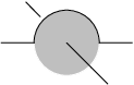
A crossing change is an operation on knots that allows us to untie every knot in finitely many steps. We say that two knots differ by a crossing change, if they are related by a strand passage operation along an embedded disc with one singularity, as illustrated in figure 1. The Gordian distance between two knots is the least number of crossing changes needed to transform one knot into the other.

The Gordian distance gives rise to a simplicial complex, the Gordian complex of knots: every isotopy class of smooth oriented knots in corresponds to a vertex. Two vertices are connected by an edge, if the corresponding knots have Gordian distance one. Similarly, an -simplex of the Gordian complex is a set of knots whose pairwise Gordian distance is one. The structure of the Gordian complex is rather complicated. As Gambaudo and Ghys proved in [2], it contains quasi-isometric embeddings of high rank grids. Moreover, every edge of the Gordian complex is contained in a simplex of infinite dimension (see [5]).
Given two knots of Gordian distance two, we may ask how many knots are ‘between’ them. Quite surprisingly, the answer is ‘infinitely many’, as was recently shown in [1]. This can be strengthened a lot.
Theorem 1.
Let be a natural number and any knot. For every pair of knots and of Gordian distance two, there exists a knot with the following properties:
- (1)
the Gordian distance between and , is one,
- (2)
all Vassiliev invariants of of order less than or equal to coincide with those of .
Theorem 1 also provides a generalisation of Ohyama’s result ([6]), who showed that every finite set of Vassiliev invariants can be realised by an unknotting number one knot. In the next section, we prove the special case of theorem 1; the general case is proved in the third section.
2. The Casson invariant of Knots
The second coefficient of the Conway polynomial is called the Casson invariant of knots. It is the unique Vassiliev invariant of order two on knots, up to multiplication by a constant. The following skein relation provides an effective way of computing :
Here denotes the linking number of a two component link .
Proof of theorem 1, for .
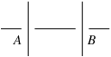
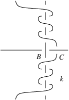
Let , be two knots of Gordian distance two. By a standard argument, has a diagram with two neighbouring crossings and , as shown in figure 2, such that a simultaneous crossing change at and transforms into . For the moment, we assume that the crossing is positive. Changing the section of , as shown in figure 3, with a certain number of half-twists above and below the crossing , we define a new knot , which is ‘between’ and . Indeed, a crossing change at transforms into , whereas a crossing change at transforms into . We note that is a negative crossing, since was a positive crossing.
Applying the skein relation for the Casson invariant at the crossing of , we get
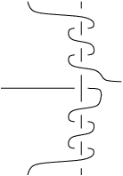
where is the two component link shown in figure 4 (the smoothing must be like this, since the crossing is negative). Varying the number of positive (or negative) half-twists, we can arrange
for any given integer . (The two ‘slalom strands’ belong to different components of , whence the vertical strand links with precisely one of the two ‘slalom strands’. Thus we can vary the linking number of , as we like.) In case is a negative crossing, we may apply an analogous construction. This proves the special case of theorem 1.
∎
3. -moves and Vassiliev invariants
The proof of Theorem 1 involves Vassiliev invariants and certain -moves, which were defined by K. Habiro in [3] (see also [4]). A -move is simply a crossing change. For , there exist -moves and special -moves. We will only use the latter. A special -move is defined diagrammatically in figure 5 (the small loop with an arrow should be ignored at this point). It takes place in a section with endpoints or strands, respectively. The strands are numbered from to and are all connected outside the indicated section, since they belong to one knot . Going along according to its orientation, starting at the first strand, we encounter the other strands in a certain order which depends on how the strands are connected outside the indicated section. This order defines a permutation, say , of the numbers 2, 3,, n+1.


In [8], Y. Ohyama and T. Tsukamoto explain the effect of a -move on Vassiliev invariants of order . Their result ([8], theorem 1.2) implies the following:
- (1)
A -move does not change the values of Vassiliev invariants of order less than .
- (2)
Let and be two knots which differ by one -move, and any Vassiliev invariant of order . Then depends only on the permutation defined by the cyclic order of the strands of the section where the -move takes place, and on the product of the signs of the crossings , , ,, (see figure 5).
The last statement of (2) follows from the proof of theorem 1.2 in [8].
We will use a slightly modified version of a special -move, as shown in figure 6. It is actually equivalent to a special -move, as we can see by dragging one end of the second strand in figure 5 along the small loop, in direction indicated by the arrow. This operation relates the two diagrams of figure 5 with those of figure 6.


Proof of theorem 1.
Let , be two fixed knots of Gordian distance two, as before. By the result of the preceding section, the case of theorem 1 is already settled: there exists a knot with any prescribed Casson invariant and . Now let us assume that theorem 1 is true for , , i.e. for any given knot , there exists a knot , such that:
- (1)
,
- (2)
all Vassiliev invariants of of order less than or equal to coincide with those of .
We will build a new knot that meets condition (2), for .
Again, by a standard argument, has a diagram with a section as shown in figure 7, with distinguished spots and , where crossing changes should take place to obtain and , respectively. In this section, we add single arcs between the two spots and , in an arbitrary way, so that we obtain a section where we can apply a special -move, as shown at the top of figure 6.

Going along the knot according to its orientation, starting at the leftmost strand, we encounter the other strands in a certain order, which again defines a permutation . We claim that we can easily change the order of two strands. This is obvious, except for the case of two strands , belonging to two different clasps, as shown at the top of figure 8 (the middle arcs are omitted here). By applying regular isotopy only, we can transform the indicated section into the section at the bottom of the figure. We observe that the order of the strands , is reversed, there. Moreover, a crossing change at the clasps involving or yields the same knots as before.


Hence we may assume that we encounter the strands of figure 6 in an order corresponding to a fixed prescribed permutation .
Applying the special -move of figure 6, we obtain a knot which is still a neighbour of and in the Gordian complex of knots: . In order to arrange the Vassiliev invariants of order of , we must invoke Habiro’s theorem.
Theorem 2 (Habiro [4]).
Two knots have the same Vassiliev invariants up to order , if, and only if, they are related by a finite sequence of -moves.
Remark.
The statement of theorem 2 remains true if we replace -moves by special -moves, since these moves are equivalent (see e.g. [7]).
Hence, in our situation, the two knots and are related by a finite sequence of special -moves. By Ohyama and Tsukamoto’s result ([8]), every single -move changes Vassiliev invariants of order in a way that only depends on the cyclic permutation defined by the outer connections and a product of signs of certain crossings. By the above observation on the permutation of strands, we can imitate this pattern in our -move from to . Repeating this procedure for every -move in the sequence from to , we end up with a knot whose Vassiliev invariants of order up to coincide with those of . This completes the proof of theorem 1. ∎
References
- [1] S. Baader: Note on crossing changes, Q. J. Math. 57 (2006), 139-142.
- [2] J.-M. Gambaudo, E. Ghys: Braids and signatures, Bull. Soc. Math. France 133 (2005), no. 4, 541-579.
- [3] K. Habiro: Master thesis, University of Tokyo (1994).
- [4] K. Habiro: Claspers and finite type invariants of links, Geom. Topol. 4 (2000), 1-83.
- [5] M. Hirasawa, Y. Uchida: The Gordian complex of knots, J. Knot Theory Ramifications 11 (2002), no. 3, 363-368.
- [6] Y. Ohyama: Web diagrams and realization of Vassiliev invariants by knots, J. Knot Theory Ramifications 9 (2000), no. 5, 693-701.
- [7] Y. Ohyama, K. Taniyama, S. Yamada: Realization of Vassiliev invariants by unknotting number one knots, Tokyo J. Math 25 (2002), no. 1, 17-31.
- [8] Y. Ohyama, T. Tsukamoto: On Habiro’s -moves and Vassiliev invariants of order , J. Knot Theory Ramifications 8 (1999), no. 2, 15-26.
Department of Mathematics, ETH Zürich, Switzerland
sebastian.baader@math.ethz.ch