跳到论文正文
W Papers独立论文阅读器 arXiv:math/0703645 论文正文 计算阅读时间 · 0%
引用这篇论文根据当前论文元数据生成,正式投稿前建议核对。


License: Assumed arXiv.org perpetual non-exclusive license
arXiv:math/0703645v2 [math.DG] 15 Apr 2008

Cyclic and ruled Lagrangian surfaces in complex Euclidean space

Henri Anciaux    Pascal Romon
Abstract

We study those Lagrangian surfaces in complex Euclidean space which are foliated by circles or by straight lines. The former, which we call cyclic, come in three types, each one being described by means of, respectively, a planar curve, a Legendrian curve in the 3-sphere or a Legendrian curve in the anti-de Sitter 3-space. We describe ruled Lagrangian surfaces and characterize the cyclic and ruled Lagrangian surfaces which are solutions to the self-similar equation of the Mean Curvature Flow. Finally, we give a partial result in the case of Hamiltonian stationary cyclic surfaces.

Keywords: Lagrangian surfaces; circle foliation; Mean Curvature Flow; Hamiltonian Stationary
2000 MSC: 53D12 (Primary) 53C42 (Secondary)

Introduction

In this paper, we classify the Lagrangian surfaces of ℂ2\mathbb{C}^{2} which are foliated either by round circles (henceforth called cyclic surfaces) or by straight lines (ruled surfaces). This completes a former paper of the authors together with Ildefonso Castro [ACR] in which all Lagrangian submanifolds of ℝ2​n≃ℂn\mathbb{R}^{2n}\simeq\mathbb{C}^{n}, with n≥3n\geq 3, which are foliated by round (n−1)(n-1)-spheres were characterized. The reason for the lower bound on the dimension was the following: since the submanifold is Lagrangian, any spherical leaf must be isotropic; when the dimension of this leaf is at least two, it spans a linear space which is itself Lagrangian. This observation simplifies the structure of the problem, roughly speaking by reducing the underlying group structure from S​O​(2​n)SO(2n) to U⁡(n)U(n). However this reduction no longer holds in dimension two, see for instance the Lagrangian cylinder 𝕊1×ℒ{\mathbb{S}}^{1}\times\mathcal{L} where ℒ\mathcal{L} is a real line of ℂ{\mathbb{C}}: this (Lagrangian) surface is foliated by circles which are contained in non-Lagrangian (actually complex) planes. Other examples are the Hopf tori studied by Pinkall in [P]. As expected the situation is richer in dimension two, and actually cyclic Lagrangian surfaces come in three families, each one being described by means of, respectively, a planar curve, a Legendrian curve in the 3-sphere or a Legendrian curve in the anti de Sitter 3-space (Theorems 1 and 2). In the following, they will be denoted as type I, II and III surfaces.

In Section 1 we classify the cyclic Lagrangian surfaces when all the centers of the circles coincide. We call those surfaces centered cyclic. In Section 2 we treat the general case which amounts to adding a convenient translation term. In Section 3 we apply this characterization to finding self-similar cyclic surfaces, that is those surfaces which are solutions of the following elliptic PDE:

H+λ​X⟂=0,H+\lambda X^{\perp}=0,

where HH denotes the mean curvature vector of the surface and X⟂X^{\perp} the normal component of its position vector. The case of positive (resp. negative) λ\lambda corresponds to the case of a self-shrinking (resp. self-expanding) soliton of the Mean Curvature Flow (see [A]). We show that a self-similar Lagrangian cyclic surface is either a centered surface of type I as described in [A] or the Cartesian product 𝕊1​(r)×Γ{\mathbb{S}}^{1}(r)\times\Gamma of a circle 𝕊1​(r){\mathbb{S}}^{1}(r) with a planar self-shrinking curve Γ\Gamma. Such curves have been studied in detail in [AL].

Section 4 is devoted to the Hamiltonian stationary equation. A Lagrangian surface is said to be Hamiltonian stationary if its area is critical for compactly supported Hamiltonian variations. Such a surface is characterized by the fact that its Lagrangian angle β\beta is harmonic with respect to the induced metric (cf Section 4 for more details). We prove that both in types I and II cases, Hamiltonian stationary surfaces must be centered, and we describe them. The study of the type III appears to be extremely difficult to handle by manual computation, however we conjecture that Hamiltonian stationary type III surfaces are again centered. Examples of such surfaces are described explicitly in [CC].

Finally we give in the last Section a description of ruled Lagrangian surfaces (notably self-similar ones) using an analogous method, recovering more simply a known result from Blair [B].

Acknowledgment: the Authors wish to thank Ildefonso Castro for pointing out a better approach to type III surfaces due to Chen and himself [CC].

1 Centered cyclic Lagrangian surfaces

Let Σ\Sigma a surface of ℝ4\mathbb{R}^{4} foliated by circles with common center located at the origin of ℝ4\mathbb{R}^{4}. Locally, Σ\Sigma may be parametrized by the following immersion:

X:I×ℝ/2​π​ℤ→ℝ4(s,t)↦r⁡(s)​(e1​(s)​cos⁡t+e2​(s)​sin⁡t),\begin{array}[]{cccl}X:&I\times\mathbb{R}/2\pi\mathbb{Z}&\to&\mathbb{R}^{4}\\ &(s,t)&\mapsto&r(s)(e_{1}(s)\cos t+e_{2}(s)\sin t),\end{array}

where r⁡(s)r(s) is a positive function and (e1​(s),e2​(s))(e_{1}(s),e_{2}(s)) is an orthonormal basis of the plane containing our circle.

From now on we shall assume that Σ\Sigma is Lagrangian with respect with some complex structure JJ. We will often identify ℝ4\mathbb{R}^{4} with ℂ2\mathbb{C}^{2} in such a way that JJ is the complex multiplication by ii. Denote by K:=⟨e1,J​e2⟩=−⟨e1,J​e2⟩K:=\langle e_{1},Je_{2}\rangle=-\langle e_{1},Je_{2}\rangle the Kähler angle of the plane e1∧e2e_{1}\wedge e_{2}. Note that the vanishing of KK means that e1∧e2e_{1}\wedge e_{2} is also Lagrangian. In this case the analysis done in [ACR] holds and XX takes the following form: X⁡(s,t)=r⁡(s)​ei​ϕ​(s)​(cos⁡t,sin⁡t)X(s,t)=r(s)e^{i\phi(s)}(\cos t,\sin t) making use of the above identification.

Denoting by subscripts the partial derivatives (the prime corresponding also to the derivative in ss for functions of just one variable), the Lagrangian assumption is equivalent to ⟨Xs,J​Xt⟩=0\langle X_{s},JX_{t}\rangle=0. Since

Xs=r′​(e1​cos⁡t+e2​sin⁡t)+r⁡(e1′​cos⁡t+e2′​sin⁡t)X_{s}=r^{\prime}(e_{1}\cos t+e_{2}\sin t)+r(e^{\prime}_{1}\cos t+e^{\prime}_{2}\sin t)
Xt=r⁡(e2​cos⁡t−e1​sin⁡t),X_{t}=r(e_{2}\cos t-e_{1}\sin t),

we see that

⟨Xs,J​Xt⟩\displaystyle\langle X_{s},JX_{t}\rangle =\displaystyle= r​r′​(K​cos2⁡t+K​sin2⁡t)+r2​(cos2⁡t⁡⟨e1′,J​e2⟩−sin2⁡t⁡⟨e2′,J​e1⟩)\displaystyle rr^{\prime}(K\cos^{2}t+K\sin^{2}t)+r^{2}\left(\cos^{2}t\langle e^{\prime}_{1},Je_{2}\rangle-\sin^{2}t\langle e^{\prime}_{2},Je_{1}\rangle\right)
+r2​cos⁡t​sin⁡t⁡(⟨e2′,J​e2⟩−⟨e1′,J​e1⟩)\displaystyle+r^{2}\cos t\sin t\left(\langle e^{\prime}_{2},Je_{2}\rangle-\langle e^{\prime}_{1},Je_{1}\rangle\right)
=\displaystyle= r​r′​K+r22​(⟨e1′,J​e2⟩−⟨e2′,J​e1⟩)\displaystyle rr^{\prime}K+\frac{r^{2}}{2}\left(\left\langle e_{1}^{\prime},Je_{2}\right\rangle-\langle e^{\prime}_{2},Je_{1}\rangle\right)
+r2​cos⁡2​t2​(⟨e1′,J​e2⟩+⟨e2′,J​e1⟩)\displaystyle+\frac{r^{2}\cos 2t}{2}\left(\langle e^{\prime}_{1},Je_{2}\rangle+\langle e^{\prime}_{2},Je_{1}\rangle\right)
+r2​sin⁡2​t2​(⟨e2′,J​e2⟩−⟨e1′,J​e1⟩)\displaystyle+\frac{r^{2}\sin 2t}{2}\left(\langle e^{\prime}_{2},Je_{2}\rangle-\langle e^{\prime}_{1},Je_{1}\rangle\right)
=\displaystyle= 2​r​r′​K+r2​K′2+r2​cos⁡2​t2​(⟨e1′,J​e2⟩+⟨e2′,J​e1⟩)\displaystyle\frac{2rr^{\prime}K+r^{2}K^{\prime}}{2}+\frac{r^{2}\cos 2t}{2}\left(\langle e^{\prime}_{1},Je_{2}\rangle+\langle e^{\prime}_{2},Je_{1}\rangle\right)
+r2​sin⁡2​t2​(⟨e2′,J​e2⟩−⟨e1′,J​e1⟩)\displaystyle+\frac{r^{2}\sin 2t}{2}\left(\langle e^{\prime}_{2},Je_{2}\rangle-\langle e^{\prime}_{1},Je_{1}\rangle\right)

which holds for all tt. The vanishing of the constant term implies that r2​K=Cr^{2}K=C for some real constant CC. If this constant vanishes, we recover the case K=0K=0 mentioned above and treated in [ACR] (cf also [A]), so we may assume that C≠0C\neq 0. Thus rr is completely determined by KK, and both are non zero.

The two remaining conditions are

⟨e1′,J​e2⟩=−⟨e2′,J​e1⟩,⟨e1′,J​e1⟩=⟨e2′,J​e2⟩.\langle e^{\prime}_{1},Je_{2}\rangle=-\langle e^{\prime}_{2},Je_{1}\rangle\;,\quad\langle e^{\prime}_{1},Je_{1}\rangle=\langle e^{\prime}_{2},Je_{2}\rangle. (1)

In order to make sense of these, we will identify ℝ4\mathbb{R}^{4} with ℍ\mathbb{H}, in such a way that the complex structure is given by the left multiplication by the quaternion ii. Then any element in S​O​(4)SO(4) can be written as x↦p​x​q−1x\mapsto pxq^{-1} where p,qp,q are two unit quaternions. Notice that right multiplication by q−1q^{-1} corresponds exactly to the elements of S​U​(2)SU(2). Since S​O​(4)SO(4) acts transitively on pairs of orthonormal vectors, we may write e1e_{1} and e2e_{2} as the respective images of 11 and ii, so that e1=p​q−1e_{1}=pq^{-1} and e2=p​i​q−1e_{2}=piq^{-1}. Note that (p,q)(p,q) is not uniquely determined; rather we have a gauge freedom by right multiplication by ei​θe^{i\theta} on (p,q)(p,q). Finally, we may assume if needed that q⁡(0)q(0) takes any prescribed value, since we consider surfaces up to U⁡(2)U(2) congruence.

Then the conditions in (1) read as

{⟨p′​q−1−p​q−1​q′​q−1,i​p​i​q−1⟩+⟨p′​i​q−1−p​i​q−1​q′​q−1,i​p​q−1⟩=0⟨p′​q−1−p​q−1​q′​q−1,i​p​q​p​q−1⟩−⟨p′​i​q−1−p​i​q−1​q′​q−1,i​p​i​q−1⟩=0\left\{\begin{array}[]{l}\left\langle p^{\prime}q^{-1}-pq^{-1}q^{\prime}q^{-1},ipiq^{-1}\right\rangle+\left\langle p^{\prime}iq^{-1}-piq^{-1}q^{\prime}q^{-1},ipq^{-1}\right\rangle=0\\ \left\langle p^{\prime}q^{-1}-pq^{-1}q^{\prime}q^{-1},ipqpq^{-1}\right\rangle-\left\langle p^{\prime}iq^{-1}-piq^{-1}q^{\prime}q^{-1},ipiq^{-1}\right\rangle=0\end{array}\right.

so, multiplying on the left by p−1p^{-1} and the right by qq, and further by ii on the left in the second bracket,

{⟨p−1​p′−q−1​q′,p−1​i​p​i⟩−⟨p−1​p′+i​q−1​q′​i,p−1​i​p​i⟩=0⟨p−1​p′−q−1​q′,p−1​i​p⟩−⟨p−1​p′+i​q−1​q′​i,p−1​i​p⟩=0\left\{\begin{array}[]{l}\left\langle p^{-1}p^{\prime}-q^{-1}q^{\prime},p^{-1}ipi\right\rangle-\left\langle p^{-1}p^{\prime}+iq^{-1}q^{\prime}i,p^{-1}ipi\right\rangle=0\\ \left\langle p^{-1}p^{\prime}-q^{-1}q^{\prime},p^{-1}ip\right\rangle-\left\langle p^{-1}p^{\prime}+iq^{-1}q^{\prime}i,p^{-1}ip\right\rangle=0\end{array}\right.

that is

{⟨q−1​q′+i​q−1​q′​i,p−1​i​p​i⟩=0⟨q−1​q′+i​q−1​q′​i,p−1​i​p⟩=0.\left\{\begin{array}[]{l}\left\langle q^{-1}q^{\prime}+iq^{-1}q^{\prime}i,p^{-1}ipi\right\rangle=0\\ \left\langle q^{-1}q^{\prime}+iq^{-1}q^{\prime}i,p^{-1}ip\right\rangle=0.\end{array}\right.

Splitting and multiplying left and right by ii in the second bracket yields

{⟨q−1​q′,p−1​i​p​i⟩−⟨q−1​q′,i​p−1​i​p⟩=0⟨q−1​q′,p−1​i​p⟩+⟨q−1​q′,i​p−1​i​p​i⟩=0\left\{\begin{array}[]{l}\left\langle q^{-1}q^{\prime},p^{-1}ipi\right\rangle-\left\langle q^{-1}q^{\prime},ip^{-1}ip\right\rangle=0\\ \left\langle q^{-1}q^{\prime},p^{-1}ip\right\rangle+\left\langle q^{-1}q^{\prime},ip^{-1}ipi\right\rangle=0\end{array}\right.
{⟨q−1​q′,p−1​i​p​i−i​p−1​i​p⟩=0⟨q−1​q′,p−1​i​p+i​p−1​i​p​i⟩=0\left\{\begin{array}[]{l}\left\langle q^{-1}q^{\prime},p^{-1}ipi-ip^{-1}ip\right\rangle=0\\ \left\langle q^{-1}q^{\prime},p^{-1}ip+ip^{-1}ipi\right\rangle=0\end{array}\right.

Writing p=p0+i​p1+j​p2+k​p3p=p_{0}+ip_{1}+jp_{2}+kp_{3} we have

u:=p−1​i​p​i−i​p−1​i​p=4​(p0​p2+p1​p3)​j−4​(p1​p2−p0​p3)​ku:=p^{-1}ipi-ip^{-1}ip=4(p_{0}p_{2}+p_{1}p_{3})j-4(p_{1}p_{2}-p_{0}p_{3})k

and

v:=p−1​i​p+i​p−1​i​p​i=−u​i=4​(p1​p2−p0​p3)​j+4​(p0​p2+p1​p3)​k.v:=p^{-1}ip+ip^{-1}ipi=-ui=4(p_{1}p_{2}-p_{0}p_{3})j+4(p_{0}p_{2}+p_{1}p_{3})k.

The two right-hand vectors u,vu,v lie in Span⁡(j,k)\mathrm{Span}(j,k) and are either linearly independent (over ℝ\mathbb{R}) or both zero. So we have two cases:

  • ∙\bullet

    u=v=0u=v=0, i.e.

    0=(p0​p2+p1​p3)2+(p1​p2−p0​p3)2=(p02+p12)​(p22+p32)0=(p_{0}p_{2}+p_{1}p_{3})^{2}+(p_{1}p_{2}-p_{0}p_{3})^{2}=(p_{0}^{2}+p_{1}^{2})(p_{2}^{2}+p_{3}^{2})

    hence pp lies in Span⁡(1,i)\mathrm{Span}(1,i) or Span⁡(j,k)\mathrm{Span}(j,k) and conditions in (1) hold. Gauging pp we may assume that p=1p=1 or p=jp=j, and the Kähler angle is then K=−1K=-1 or K=+1K=+1 respectively, so that the radius rr remains constant (and we may as well assume r=1r=1). This case corresponds to Hopf surfaces [P], i.e. inverse images of a curve by the Hopf fibration 𝕊3→𝕊2{\mathbb{S}}^{3}\rightarrow{\mathbb{S}}^{2}. After a possible change of variable in tt (replacing tt by t+φ⁡(s)t+\varphi(s) for some function φ\varphi), we may assume that the curve s↦e1​(s)s\mapsto e_{1}(s) is Legendrian.

  • ∙\bullet

    u,vu,v are independent vectors and span j,kj,k, thus forcing q−1​q′q^{-1}q^{\prime} to lie in Span⁡(1,i)∩Im​ℍ\mathrm{Span}(1,i)\cap\mathrm{Im}{\mathbb{H}}; using gauge action, we may assume that qq is constant, and up to congruence write q=1q=1. Reverting to complex coordinates, e1=p=γ1+γ2​j≃(γ1,γ2)∈𝕊3⊂ℂ2e_{1}=p=\gamma_{1}+\gamma_{2}j\simeq(\gamma_{1},\gamma_{2})\in{\mathbb{S}}^{3}\subset\mathbb{C}^{2} and e2=p​i≃(i​γ1,−i​γ2)e_{2}=pi\simeq(i\gamma_{1},-i\gamma_{2}), while K=|γ2|2−|γ1|2≠0K=|\gamma_{2}|^{2}-|\gamma_{1}|^{2}\neq 0. We may normalize, assuming that K>0K>0 (if K<0K<0 pick the opposite orientation on the surface) and set (α1,α2):=1K​(γ1,γ2)(\alpha_{1},\alpha_{2}):=\frac{1}{\sqrt{K}}(\gamma_{1},\gamma_{2}), so that

    X=CK​(γ1​(s)​ei​t,γ2​(s)​e−i​t)=C​(α1​ei​t,α2​e−i​t)X=\frac{\sqrt{C}}{\sqrt{K}}(\gamma_{1}(s)e^{it},\gamma_{2}(s)e^{-it})=\sqrt{C}(\alpha_{1}e^{it},\alpha_{2}e^{-it})

    with |α1|2−|α2|2=−1|\alpha_{1}|^{2}-|\alpha_{2}|^{2}=-1, i.e. (α1,α2)(\alpha_{1},\alpha_{2}) lies in ℍ13{\mathbb{H}}_{1}^{3}, the unit anti-De Sitter space. Again, up to a change in variable, we have a Legendrian curve for the indefinite metric in ℂ1,1\mathbb{C}^{1,1}, i.e. ⟨α1′,i​α1⟩−⟨α2′,i​α2⟩=0\left\langle\alpha_{1}^{\prime},i\alpha_{1}\right\rangle-\left\langle\alpha_{2}^{\prime},i\alpha_{2}\right\rangle=0 (see [CLU] or [CC]).

Summing up, we have proved the following

Theorem 1

A centered cyclic Lagrangian surface may be locally parametrized, up to U⁡(2)U(2) congruence, by one the following immersions:

Type I

(complex extensors):

X:I×ℝ/2​π​ℤ→ℂ2(s,t)↦r⁡(s)​ei​ϕ​(s)​(cos⁡t,sin⁡t)\begin{array}[]{cccl}X:&I\times\mathbb{R}/2\pi\mathbb{Z}&\to&\mathbb{C}^{2}\\ &(s,t)&\mapsto&r(s)e^{i\phi(s)}(\cos t,\sin t)\end{array}
Type II

(Hopf type):

X:I×ℝ/2​π​ℤ→ℂ2(s,t)↦c​ei​t​(γ1​(s),γ2​(s))\begin{array}[]{cccl}X:&I\times\mathbb{R}/2\pi\mathbb{Z}&\to&\mathbb{C}^{2}\\ &(s,t)&\mapsto&ce^{it}(\gamma_{1}(s),\gamma_{2}(s))\end{array}

where γ=(γ1,γ2)\gamma=(\gamma_{1},\gamma_{2}) is any Legendrian curve of 𝕊3\mathbb{S}^{3} and cc is a real constant,

Type III

(De Sitter type)

X:I×ℝ/2​π​ℤ→ℂ2(s,t)↦c⁡(α1​(s)​ei​t,α2​(s)​e−i​t)\begin{array}[]{cccl}X:&I\times\mathbb{R}/2\pi\mathbb{Z}&\to&\mathbb{C}^{2}\\ &(s,t)&\mapsto&c\left(\alpha_{1}(s)e^{it},\alpha_{2}(s)e^{-it}\right)\end{array}

where α=(α1,α2)\alpha=(\alpha_{1},\alpha_{2}) is any Legendrian curve in the unit anti-De Sitter space ℍ13{\mathbb{H}}_{1}^{3} and cc is a real constant.

Remark 1

This analysis applies as well if we do not assume that XX is an immersion but only has an isotropic image fibered by circles (we did not use the immersion hypothesis). So the same conclusion holds and will be used in the next Section.

Remark 2

Type I surfaces are a particular case of a class of Lagrangian immersions which has been first described in [C1] where they were called complex extensors.

Remark 3

In the type III case, it may happen that KK is identically ±1\pm 1. Then we fall back on type II with a Legendrian curve that actually reduces to a single point. The image of XX is therefore a circle (lying in a complex plane).

2 The general case

We now consider a surface Σ\Sigma of ℝ4\mathbb{R}^{4} which is foliated by circles. Locally, Σ\Sigma may be parametrized by the following immersion (identifying as usual ℝ4\mathbb{R}^{4} with ℂ2\mathbb{C}^{2}):

Y:I×ℝ/2​π​ℤ→ℂ2(s,t)↦X⁡(s,t)+V⁡(s),\begin{array}[]{cccl}Y:&I\times\mathbb{R}/2\pi\mathbb{Z}&\to&\mathbb{C}^{2}\\ &(s,t)&\mapsto&X(s,t)+V(s),\end{array}

where V⁡(s)V(s) is a ℂ2\mathbb{C}^{2}-valued function, and X⁡(s,t)=r⁡(s)​(e1​(s)​cos⁡t+e2​(s)​sin⁡t)X(s,t)=r(s)(e_{1}(s)\cos t+e_{2}(s)\sin t) is a centered surface as in the previous section. Note that we do not assume a priori that XX is Lagrangian nor that it is always an immersion.

As we have Yt=XtY_{t}=X_{t} and Ys=Xs+V′Y_{s}=X_{s}+V^{\prime}, the assumption that YY is Lagrangian leads to:

0=⟨Ys,J​Yt⟩=⟨Xs,J​Xt⟩+⟨V′,J​Xt⟩=⟨Xs,JXt⟩+rcost⟨V′,Je2⟩−rsint⟨V′,1⟩\begin{array}[]{ccl}0&=&\langle Y_{s},JY_{t}\rangle=\langle X_{s},JX_{t}\rangle+\langle V^{\prime},JX_{t}\rangle\\ &=&\langle X_{s},JX_{t}\rangle+r\cos t\langle V^{\prime},Je_{2}\rangle-r\sin t\langle V^{\prime},_{1}\rangle\end{array}

Recall from the previous section that ⟨Xs,J​Xt⟩\langle X_{s},JX_{t}\rangle contains only terms in cos⁡2​t\cos 2t and sin⁡2​t\sin 2t and a term independent from tt. Thus the immersion YY is Lagrangian if and only if: (i) XX is cyclic isotropic (cf Remark 1), and (ii) V′V^{\prime} belongs to the symplectic orthogonal of Span⁡(e1,e2)\mathrm{Span}(e_{1},e_{2}). Using Theorem 1 we infer:

  • •

    for type I surfaces, Span⁡(e1,e2)=Span⁡(ei​ϕ​(1,0),ei​ϕ​(0,1))\mathrm{Span}(e_{1},e_{2})=\mathrm{Span}(e^{i\phi}(1,0),e^{i\phi}(0,1)) is Lagrangian, so its symplectic orthogonal is itself; hence V′​(s)=ei​ϕ​(s)​(W1​(s),W2​(s))V^{\prime}(s)=e^{i\phi(s)}(W_{1}(s),W_{2}(s)) for some real-valued functions W1,W2W_{1},W_{2};

  • •

    for type II surfaces, Span⁡(e1,e2)\mathrm{Span}(e_{1},e_{2}) is a complex line, so its symplectic orthogonal is the same as its Riemannian orthogonal, which is

    Span⁡((γ¯2,−γ¯1),(i​γ¯2,−i​γ¯1));\mathrm{Span}((\bar{\gamma}_{2},-\bar{\gamma}_{1}),(i\bar{\gamma}_{2},-i\bar{\gamma}_{1}));

    V′V^{\prime} is determined analogously;

  • •

    for type III surfaces, one can check than a basis of the symplectic orthogonal is (f1,f2)(f_{1},f_{2}), where f1=(|α2|2,α1​α2)f_{1}=(|\alpha_{2}|^{2},\alpha_{1}\alpha_{2}), f2=(i​|α2|2,−i​α1​α2)f_{2}=(i|\alpha_{2}|^{2},-i\alpha_{1}\alpha_{2}).

So we conclude this section by the

Theorem 2

A cyclic Lagrangian surface may be locally parametrized, up to U⁡(2)U(2) congruence, by one the following immersions:

Type I
Y:I×ℝ/2​π​ℤ→ℂ2(s,t)↦r⁡(s)​ei​ϕ​(s)​(cos⁡t,sin⁡t)+∫s0sei​ϕ​(u)​(W1​(u),W2​(u))​𝑑u\begin{array}[]{cccl}Y:&I\times\mathbb{R}/2\pi\mathbb{Z}&\to&\mathbb{C}^{2}\\ &(s,t)&\mapsto&r(s)e^{i\phi(s)}(\cos t,\sin t)+\int_{s_{0}}^{s}e^{i\phi(u)}(W_{1}(u),W_{2}(u))du\end{array}

where W1,W2W_{1},W_{2} are real valued; in particular when ϕ\phi is constant, YY stays within the Lagrangian plane Span⁡(ei​ϕ​(1,0),ei​ϕ​(0,1))\mathrm{Span}(e^{i\phi}(1,0),e^{i\phi}(0,1));

Type II
Y:I×ℝ/2​π​ℤ→ℂ2(s,t)↦c⁡(γ1​(s)​ei​t,γ2​(s)​ei​t)+∫s0sW⁡(u)​(γ¯2​(u),−γ¯1​(u))​𝑑u\begin{array}[]{cccl}Y:&I\times\mathbb{R}/2\pi\mathbb{Z}&\to&\mathbb{C}^{2}\\ &(s,t)&\mapsto&c\left(\gamma_{1}(s)e^{it},\gamma_{2}(s)e^{it}\right)+\int_{s_{0}}^{s}W(u)(\bar{\gamma}_{2}(u),-\bar{\gamma}_{1}(u))du\end{array}

where γ=(γ1,γ2)\gamma=(\gamma_{1},\gamma_{2}) is any Legendrian curve of 𝕊3\mathbb{S}^{3}, cc is a real constant and WW a complex valued function; in particular if γ\gamma is constant, then up to congruence, we may assume γ=(1,0)\gamma=(1,0) and the immersion becomes Y⁡(s,t)=(c​ei​t,V2​(s))Y(s,t)=(ce^{it},V_{2}(s)). Thus the immersed surface is a Cartesian product of a circle with a planar curve;

Type III
Y:I×ℝ/2​π​ℤ→ℂ2(s,t)↦c⁡(α1​(s)​ei​t,α2​(s)​e−i​t)+∫s0s(W​|α2|2,W¯​α1​α2)​𝑑u\begin{array}[]{cccl}Y:&I\times\mathbb{R}/2\pi\mathbb{Z}&\to&\mathbb{C}^{2}\\ &(s,t)&\mapsto&c\left(\alpha_{1}(s)e^{it},\alpha_{2}(s)e^{-it}\right)+\int_{s_{0}}^{s}(W|\alpha_{2}|^{2},\bar{W}\alpha_{1}\alpha_{2})du\end{array}

where α=(α1,α2)\alpha=(\alpha_{1},\alpha_{2}) is any Legendrian curve in the unit anti-De Sitter space ℍ13{\mathbb{H}}_{1}^{3}, cc is a real constant and WW a complex valued function.

Remark 4

In the type II case, if the curve (γ1,γ2)(\gamma_{1},\gamma_{2}) is in addition regular, we may assume that it is parametrized by arc length and another basis of the orthogonal space to Span⁡(e1,e2)\mathrm{Span}(e_{1},e_{2}) is ((γ1′,γ2′),(i​γ1′,i​γ2′))\left((\gamma^{\prime}_{1},\gamma^{\prime}_{2}),(i\gamma^{\prime}_{1},i\gamma^{\prime}_{2})\right), so that the immersion may take the alternative form:

Y⁡(s,t)=(γ1​(s)​ei​t,γ2​(s)​ei​t)+∫s0sW⁡(u)​(γ1′​(u),γ2′​(u))​𝑑u.Y(s,t)=(\gamma_{1}(s)e^{it},\gamma_{2}(s)e^{it})+\int_{s_{0}}^{s}W(u)(\gamma^{\prime}_{1}(u),\gamma^{\prime}_{2}(u))du.

This is a particular case of Lagrangian immersions which have been recently described in [C2]. This alternative formula will also be useful in the next sections.

3 Application to the self-similar equation

In this section we study the self-similar equation in the case of cyclic Lagrangian surfaces and prove the following:

Theorem 3

A Lagrangian cyclic surface of ℂ2{\mathbb{C}}^{2} which is a soliton of the mean curvature flow, i.e. a solution to the self-similar equation

H+λ​X⟂=0,H+\lambda X^{\perp}=0,

for some non-vanishing number λ\lambda is locally congruent to an equivariant example described in [A] (in the terminology of the present article, a centered surface of type I) or to the Cartesian product 𝕊1​(r)×Γ{\mathbb{S}}^{1}(r)\times{\Gamma} of some circle 𝕊1​(1){\mathbb{S}}^{1}(1) with a planar self-shrinking curve Γ{\Gamma}. Such curves have been studied in detail in [AL].

Proof. The proof deals with the three cyclic cases separately: we first prove that a self-similar surface of type I must be centered, thus one of the examples of [A]; then we show that there no self-similar surfaces of type II except the Clifford torus 𝕊1×𝕊1{\mathbb{S}}^{1}\times{\mathbb{S}}^{1} (which is also a type I surface) and the products of curves. Finally we see that there are no self-similar surfaces of type III at all.

Case 1: type I surfaces.

A type I surface is parametrized by an immersion of the form:

X:I×ℝ/2​π​ℤ→ℂ2(s,t)↦r⁡(s)​ei​ϕ​(s)​(cos⁡t,sin⁡t)+∫s0sei​ϕ​(u)​(W1​(u),W2​(u))​du,\begin{array}[]{clcl}X:&I\times{\mathbb{R}}/2\pi{\mathbb{Z}}&\to&{\mathbb{C}}^{2}\\ &(s,t)&\mapsto&r(s)e^{i\phi(s)}(\cos t,\sin t)+\int_{s_{0}}^{s}e^{i\phi(u)}(W_{1}(u),W_{2}(u))du,\end{array}

where r⁡(s)>0r(s)>0. Following [ACR], we shall use the following notations: γ⁡(s)=r⁡(s)​ei​ϕ​(s)\gamma(s)=r(s)e^{i\phi(s)}, and, assuming that γ\gamma is parametrized by arc length, we shall also denote γ′​(s)=ei​θ​(s)\gamma^{\prime}(s)=e^{i\theta(s)}.

We start computing the first derivatives of the immersion:

Xs=γ′​(cos⁡t,sin⁡t)+ei​ϕ​(W1,W2),Xt=γ⁡(−sin⁡t,cos⁡t),X_{s}=\gamma^{\prime}(\cos t,\sin t)+e^{i\phi}(W_{1},W_{2}),\hskip 30.00005ptX_{t}=\gamma(-\sin t,\cos t),

from which we deduce the expression of the induced metric:

E=|Xs|2=1+|W|2+2​cos⁡(θ−ϕ)​(W1​cos⁡t+W2​sin⁡t),E=|X_{s}|^{2}=1+|W|^{2}+2\cos(\theta-\phi)(W_{1}\cos t+W_{2}\sin t),
F=⟨Xs,Xt⟩=r​cos⁡(θ−ϕ)​(W2​cos⁡t−W1​sin⁡t),G=|Xt|2=r2,F=\langle X_{s},X_{t}\rangle=r\cos(\theta-\phi)(W_{2}\cos t-W_{1}\sin t),\qquad G=|X_{t}|^{2}=r^{2},

and a basis of the normal space to the surface:

Nt=i​γ​(−sin⁡t,cos⁡t),Ns=i​γ′​(cos⁡t,sin⁡t)+i​ei​ϕ​(W1,W2).N_{t}=i\gamma(-\sin t,\cos t),\hskip 30.00005ptN_{s}=i\gamma^{\prime}(\cos t,\sin t)+ie^{i\phi}(W_{1},W_{2}).

We now compute the second derivatives of the immersion, in order to calculate the mean curvature vector:

Xs​s=γ′′​(cos⁡t,sin⁡t)+i​ϕ′​ei​ϕ​(W1,W2),X_{ss}=\gamma^{\prime\prime}(\cos t,\sin t)+i\phi^{\prime}e^{i\phi}(W_{1},W_{2}),
Xs​t=γ′​(−sin⁡t,cos⁡t),Xt​t=γ⁡(−cos⁡t,−sin⁡t).X_{st}=\gamma^{\prime}(-\sin t,\cos t),\hskip 30.00005ptX_{tt}=\gamma(-\cos t,-\sin t).

This implies in particular that:

⟨Xs​s,Nt⟩=(W2​cos⁡t−W1​sin⁡t)​sin⁡(θ−ϕ),\langle X_{ss},N_{t}\rangle=(W_{2}\cos t-W_{1}\sin t)\sin(\theta-\phi),
⟨Xt​t,Nt⟩=0,⟨Xs​t,Nt⟩=r​sin⁡(θ−ϕ).\langle X_{tt},N_{t}\rangle=0,\hskip 30.00005pt\langle X_{st},N_{t}\rangle=r\sin(\theta-\phi).

On the other hand, we have:

⟨X,Nt⟩=a​cos⁡t+b​sin⁡t,\langle X,N_{t}\rangle=a\cos t+b\sin t,

where a:=⟨i​γ,∫s0sW1​(u)​ei​ϕ​(u)​𝑑u⟩a:=\langle i\gamma,\int_{s_{0}}^{s}W_{1}(u)e^{i\phi(u)}du\rangle and b:=⟨i​γ,∫s0sW2​(u)​ei​ϕ​(u)​𝑑u⟩b:=\langle i\gamma,\int_{s_{0}}^{s}W_{2}(u)e^{i\phi(u)}du\rangle.

We now assume that the immersion XX is self-similar, so there exists a non-vanishing real number λ\lambda such that:

⟨H,Nt⟩+λ⁡⟨X,Nt⟩=0,\langle H,N_{t}\rangle+\lambda\langle X,N_{t}\rangle=0,

which is equivalent to

⟨Xs​s,Nt⟩​G+⟨Xt​t,Nt⟩​E−2​⟨Xs​t,Nt⟩​F=−2​λ​(E​G−F2)​⟨X,Nt⟩.\langle X_{ss},N_{t}\rangle G+\langle X_{tt},N_{t}\rangle E-2\langle X_{st},N_{t}\rangle F=-2\lambda(EG-F^{2})\langle X,N_{t}\rangle.

In the latter expression, the left hand side term is linear in cos⁡t\cos t and sin⁡t\sin t and the right hand side term is a polynomial of order 3. Linearizing the latter, we easily see that the coefficient of cos⁡2​t\cos 2t is a​W2+b​W1aW_{2}+bW_{1} and the one of sin⁡2​t\sin 2t is a​W1−b​W2aW_{1}-bW_{2}. So either W1W_{1} and W2W_{2} vanish, or aa and bb vanish. We are going to show that actually if aa and bb vanish, then so do W1W_{1} and W2W_{2}.

We first write

a=⟨i​γ,∫s0sW1​(u)​ei​ϕ​(u)⟩=r⁡⟨i​ei​ϕ,∫s0sW1​(u)​ei​ϕ​(u)​𝑑u⟩a=\langle i\gamma,\int_{s_{0}}^{s}W_{1}(u)e^{i\phi(u)}\rangle=r\langle ie^{i\phi},\int_{s_{0}}^{s}W_{1}(u)e^{i\phi(u)}du\rangle
=r⁡(−sin⁡ϕ⁡(∫s0sW1​(u)​cos⁡ϕ⁡(u)​𝑑u)+cos⁡ϕ⁡(∫s0sW1​(u)​sin⁡ϕ⁡(u)​𝑑u))=0.=r\left(-\sin\phi\left(\int_{s_{0}}^{s}W_{1}(u)\cos\phi(u)du\right)+\cos\phi\left(\int_{s_{0}}^{s}W_{1}(u)\sin\phi(u)du\right)\right)=0.

Thus the derivative of a/ra/r with respect to ss must vanish, which yields:

ϕ′​(−cos⁡ϕ⁡(∫s0sW1​(u)​cos⁡ϕ⁡(u)​𝑑u)−sin⁡ϕ⁡(∫s0sW1​(u)​sin⁡ϕ⁡(u)​𝑑u))\phi^{\prime}\left(-\cos\phi\left(\int_{s_{0}}^{s}W_{1}(u)\cos\phi(u)du\right)-\sin\phi\left(\int_{s_{0}}^{s}W_{1}(u)\sin\phi(u)du\right)\right)
+W1​(s)​(−sin⁡ϕ​cos⁡ϕ+cos⁡ϕ​sin⁡ϕ)=0.+W_{1}(s)(-\sin\phi\cos\phi+\cos\phi\sin\phi)=0.

Now either ϕ\phi is (locally) constant, the curve γ\gamma is a straight line passing through the origin and the image of the immersion XX is a piece of a plane (cf Example 2, page 5 of [ACR]), or one can find find points around which ϕ′\phi^{\prime} does not vanish (locally again). In the latter case we get the following linear system:

{−sin⁡ϕ⁡(∫s0sW1​(u)​cos⁡ϕ⁡(u)​du)+cos⁡ϕ⁡(∫s0sW1​(u)​sin⁡ϕ⁡(u)​du)=0−cos⁡ϕ⁡(∫s0sW1​(u)​cos⁡ϕ⁡(u)​du)−sin⁡ϕ⁡(∫s0sW1​(u)​sin⁡ϕ⁡(u)​du)=0\left\{\begin{array}[]{lcc}-\sin\phi\left(\int_{s_{0}}^{s}W_{1}(u)\cos\phi(u)du\right)+\cos\phi\left(\int_{s_{0}}^{s}W_{1}(u)\sin\phi(u)du\right)&=&0\\ -\cos\phi\left(\int_{s_{0}}^{s}W_{1}(u)\cos\phi(u)du\right)-\sin\phi\left(\int_{s_{0}}^{s}W_{1}(u)\sin\phi(u)du\right)&=&0\end{array}\right.

It follows that ∫s0sW1​(u)​cos⁡ϕ⁡(u)​𝑑u\int_{s_{0}}^{s}W_{1}(u)\cos\phi(u)du and ∫s0sW1​(u)​sin⁡ϕ⁡(u)​𝑑u\int_{s_{0}}^{s}W_{1}(u)\sin\phi(u)du must vanish except on an isolated set of points of II, which in turn implies the vanishing of W1W_{1}. Analogously it can be shown that W2W_{2} vanishes as well, so finally the surface must be centered. Lagrangian, self-similar, centered surfaces have been described in detail in [A]. We only recall here that such surfaces are obtained from planar curves γ\gamma which are solutions of the following equation:

k=⟨γ,N⟩​(1|γ|2−λ),k=\langle\gamma,N\rangle\left(\frac{1}{|\gamma|^{2}}-\lambda\right),

where kk is the curvature of γ\gamma and NN its unit normal vector. This equation admits a countable family of closed solutions which is parametrised by two relatively prime numbers pp and qq subject to the condition p/q∈(1/4,1/2);p/q\in(1/4,1/2); pp is the winding number of the curve and qq is the number of maxima of its curvature. Except for the circles, none of these curves is embedded.

Case 2: type II surfaces.

As our discussion is local, we consider the two following cases: either the Legendrian curve γ\gamma is regular, or it reduces to a single point, and then the surface is a product of a circle with some plane curve. In the first case, the surface may parametrized by an immersion of the form (cf Remark 4):

X:I×ℝ/2​π​ℤ→ℂ2(s,t)↦c⁡(γ1​(s)​ei​t,γ2​(s)​ei​t)+∫s0sW⁡(u)​(γ1′,γ2′)​𝑑u\begin{array}[]{clcl}X:&I\times{\mathbb{R}}/2\pi{\mathbb{Z}}&\to&{\mathbb{C}}^{2}\\ &(s,t)&\mapsto&c(\gamma_{1}(s)e^{it},\gamma_{2}(s)e^{it})+\int_{s_{0}}^{s}W(u)(\gamma^{\prime}_{1},\gamma^{\prime}_{2})du\end{array}

where (γ1​(s),γ2​(s))(\gamma_{1}(s),\gamma_{2}(s)) is some unit speed Legendrian curve of 𝕊3{\mathbb{S}}^{3}. Without loss of generality we fix c=1c=1. We start computing the first derivatives of the immersion:

Xs=(γ1′​ei​t,γ2′​ei​t)+W⁡(γ1′,γ2′),Xt=(i​γ1​ei​t,i​γ2​ei​t),X_{s}=(\gamma^{\prime}_{1}e^{it},\gamma^{\prime}_{2}e^{it})+W(\gamma^{\prime}_{1},\gamma^{\prime}_{2}),\hskip 30.00005ptX_{t}=(i\gamma_{1}e^{it},i\gamma_{2}e^{it}),

from which we deduce the expression of the induced metric:

E=|Xs|2=1+|W|2+2​⟨W,ei​t⟩,F=⟨Xs,Xt⟩=0,G=|Xt|2=1,E=|X_{s}|^{2}=1+|W|^{2}+2\langle W,e^{it}\rangle,\qquad F=\langle X_{s},X_{t}\rangle=0,\qquad G=|X_{t}|^{2}=1,

and a basis of the normal space to the surface:

Ns=(i​γ1′​ei​t,i​γ2′​ei​t)+W⁡(i​γ1′,i​γ2′),Nt=(−γ1​ei​t,−γ2​ei​t).N_{s}=(i\gamma^{\prime}_{1}e^{it},i\gamma^{\prime}_{2}e^{it})+W(i\gamma^{\prime}_{1},i\gamma^{\prime}_{2}),\hskip 30.00005ptN_{t}=(-\gamma_{1}e^{it},-\gamma_{2}e^{it}).

We now compute the second derivatives of the immersion, in order to calculate the mean curvature vector:

Xs​s=(γ1′′​ei​t,γ2′′​ei​t)+W⁡(γ1′′,γ2′′)+W′​(γ1′,γ2′),X_{ss}=(\gamma^{\prime\prime}_{1}e^{it},\gamma^{\prime\prime}_{2}e^{it})+W(\gamma_{1}^{\prime\prime},\gamma^{\prime\prime}_{2})+W^{\prime}(\gamma^{\prime}_{1},\gamma^{\prime}_{2}),
Xs​t=(i​γ1′​ei​t,i​γ2′​ei​t),Xt​t=(−γ1​ei​t,−γ2​ei​t).X_{st}=(i\gamma^{\prime}_{1}e^{it},i\gamma^{\prime}_{2}e^{it}),\hskip 40.00006ptX_{tt}=(-\gamma_{1}e^{it},-\gamma_{2}e^{it}).

We first notice that

⟨X,Nt⟩=−1+a​cos⁡t+b​sin⁡t,\langle X,N_{t}\rangle=-1+a\cos t+b\sin t,

where aa and bb depend only on the variable ss.

On the other hand,

2​⟨H,Nt⟩=⟨Xs​s,Nt⟩E+⟨Xt​t,Nt⟩G=⟨Xs​t,Ns⟩E+⟨Xt​t,Nt⟩G2\langle H,N_{t}\rangle=\frac{\langle X_{ss},N_{t}\rangle}{E}+\frac{\langle X_{tt},N_{t}\rangle}{G}=\frac{\langle X_{st},N_{s}\rangle}{E}+\frac{\langle X_{tt},N_{t}\rangle}{G}
=1+⟨W,ei​t⟩1+|W|2+2​⟨W,ei​t⟩+1=2+|W|2+3​⟨W,ei​t⟩1+|W|2+2​⟨W,ei​t⟩.=\frac{1+\langle W,e^{it}\rangle}{1+|W|^{2}+2\langle W,e^{it}\rangle}+1=\frac{2+|W|^{2}+3\langle W,e^{it}\rangle}{1+|W|^{2}+2\langle W,e^{it}\rangle}.

Thus the equation ⟨H,Nt⟩+λ⁡⟨X,Nt⟩=0\langle H,N_{t}\rangle+\lambda\langle X,N_{t}\rangle=0 holds for some non-vanishing constant λ\lambda if and only if aa and bb vanish and |W|=1|W|=1 or W=0W=0. In particular, ⟨X,Nt⟩=−1\langle X,N_{t}\rangle=-1.

We leave to the reader the easy task to check that if WW vanishes, the immersion is self-similar if and only if ⟨γ′′,J​γ′⟩\langle\gamma^{\prime\prime},J\gamma^{\prime}\rangle vanishes, that is the curve γ\gamma has vanishing curvature and thus is a great circle. The corresponding Lagrangian surface is the Clifford torus 12​𝕊1×12​𝕊1\frac{1}{\sqrt{2}}{\mathbb{S}}^{1}\times\frac{1}{\sqrt{2}}{\mathbb{S}}^{1}. So we assume in the remainder that |W|=1|W|=1. In particular, we may write W=ei​ϕW=e^{i\phi} and W′=i​ϕ′​ei​ϕW^{\prime}=i\phi^{\prime}e^{i\phi}, where ϕ\phi is some real function of the variable ss.

We want to look at the other scalar equation ⟨H,Ns⟩+λ⁡⟨X,Ns⟩=0\langle H,N_{s}\rangle+\lambda\langle X,N_{s}\rangle=0, so we compute

⟨Xs​s,Ns⟩=⟨γ′′,J​γ′⟩​(1+|W|2)+⟨i​W,W′⟩+2​⟨W,e−i​t⟩​⟨γ′′,J​γ′⟩+⟨W′,ei​t⟩,\langle X_{ss},N_{s}\rangle=\langle\gamma^{\prime\prime},J\gamma^{\prime}\rangle(1+|W|^{2})+\langle iW,W^{\prime}\rangle+2\langle W,e^{-it}\rangle\langle\gamma^{\prime\prime},J\gamma^{\prime}\rangle+\langle W^{\prime},e^{it}\rangle,
⟨Xt​t,Ns⟩=0.\langle X_{tt},N_{s}\rangle=0.

Hence we get

2​⟨H,Ns⟩=⟨Xs​s,Ns⟩E+⟨Xt​t,Ns⟩G=⟨Xs​s,Ns⟩1+|W|2+2​⟨W,ei​t⟩+0=⟨γ′′,J​γ′⟩​(1+|W|2)+⟨i​W,W′⟩+2​⟨W,e−i​t⟩​⟨γ′′,J​γ′⟩+⟨W′,ei​t⟩1+|W|2+2​⟨W,ei​t⟩=2​⟨γ′′,J​γ′⟩+ϕ′+2​cos⁡(ϕ+t)​⟨γ′′,J​γ′⟩−ϕ′​sin⁡(ϕ−t)2+2​cos⁡(ϕ−t)=2​⟨γ′′,J​γ′⟩+ϕ′+(2​⟨γ′′,J​γ′⟩​cos⁡ϕ−ϕ′​sin⁡ϕ)​cos⁡t2​(1+cos⁡ϕ​cos⁡t+sin⁡ϕ​sin⁡t)+(−2​⟨γ′′,J​γ′⟩​sin⁡ϕ+ϕ′​cos⁡ϕ)​sin⁡t2​(1+cos⁡ϕ​cos⁡t+sin⁡ϕ​sin⁡t)\begin{array}[]{rcl}2\langle H,N_{s}\rangle&=&\displaystyle\frac{\langle X_{ss},N_{s}\rangle}{E}+\frac{\langle X_{tt},N_{s}\rangle}{G}=\frac{\langle X_{ss},N_{s}\rangle}{1+|W|^{2}+2\langle W,e^{it}\rangle}+0\\ &=&\displaystyle\frac{\langle\gamma^{\prime\prime},J\gamma^{\prime}\rangle(1+|W|^{2})+\langle iW,W^{\prime}\rangle+2\langle W,e^{-it}\rangle\langle\gamma^{\prime\prime},J\gamma^{\prime}\rangle+\langle W^{\prime},e^{it}\rangle}{1+|W|^{2}+2\langle W,e^{it}\rangle}\\ &=&\displaystyle\frac{2\langle\gamma^{\prime\prime},J\gamma^{\prime}\rangle+\phi^{\prime}+2\cos(\phi+t)\langle\gamma^{\prime\prime},J\gamma^{\prime}\rangle-\phi^{\prime}\sin(\phi-t)}{2+2\cos(\phi-t)}\\ &=&\displaystyle\frac{2\langle\gamma^{\prime\prime},J\gamma^{\prime}\rangle+\phi^{\prime}+(2\langle\gamma^{\prime\prime},J\gamma^{\prime}\rangle\cos\phi-\phi^{\prime}\sin\phi)\cos t}{2(1+\cos\phi\cos t+\sin\phi\sin t)}\\ &&+\displaystyle\frac{(-2\langle\gamma^{\prime\prime},J\gamma^{\prime}\rangle\sin\phi+\phi^{\prime}\cos\phi)\sin t}{2(1+\cos\phi\cos t+\sin\phi\sin t)}\end{array}

On the other hand, it is easy to see that ⟨X,Ns⟩\langle X,N_{s}\rangle takes the form a​cos⁡t+b​sin⁡t+ca\cos t+b\sin t+c, where aa bb and cc depend on the variable ss. This forces ⟨H,Ns⟩\langle H,N_{s}\rangle to take a simpler form and implies that

2​⟨γ′′,J​γ′⟩+ϕ′2=2​⟨γ′′,J​γ′⟩​cos⁡ϕ−ϕ′​sin⁡ϕ2​cos⁡ϕ=−2​⟨γ′′,J​γ′⟩​sin⁡ϕ+ϕ′​cos⁡ϕ2​sin⁡ϕ\frac{2\langle\gamma^{\prime\prime},J\gamma^{\prime}\rangle+\phi^{\prime}}{2}=\frac{2\langle\gamma^{\prime\prime},J\gamma^{\prime}\rangle\cos\phi-\phi^{\prime}\sin\phi}{2\cos\phi}=\frac{-2\langle\gamma^{\prime\prime},J\gamma^{\prime}\rangle\sin\phi+\phi^{\prime}\cos\phi}{2\sin\phi}

In particular we have ϕ′=−ϕ′​tan⁡ϕ\phi^{\prime}=-\phi^{\prime}\tan\phi, which implies that ϕ\phi is constant. It follows that WW is constant as well, so ⟨γ′′,J​γ′⟩\langle\gamma^{\prime\prime},J\gamma^{\prime}\rangle vanishes and the curve γ\gamma has vanishing curvature, so it is a great circle of the unit sphere. There is no loss of generality to assume that γ⁡(s)=12​(ei​s,e−i​s)\gamma(s)=\frac{1}{\sqrt{2}}(e^{is},e^{-is}). Now the immersion takes the following, explicit form:

X⁡(s,t)=12​(ei⁡(s+t),ei⁡(−s+t))+12​(−i​ei⁡(ϕ+s),i​ei⁡(ϕ−s)).X(s,t)=\frac{1}{\sqrt{2}}(e^{i(s+t)},e^{i(-s+t)})+\frac{1}{\sqrt{2}}(-ie^{i(\phi+s)},ie^{i(\phi-s)}).

But in this case it is easy to check ⟨X,Nt⟩=−1\langle X,N_{t}\rangle=-1 does not hold, so we conclude that there is no self-similar type II surface with a regular curve γ\gamma and non-vanishing WW.

It remains to treat the case of a Cartesian product 𝕊1​(r)×Γ{\mathbb{S}}^{1}(r)\times\Gamma of a circle with an arbitrary curve Γ\Gamma. It is straightforward that such a product is self-similar if and only if both curves are solutions of the equation

k+λ​⟨X,N⟩=0k+\lambda\langle X,N\rangle=0

for the same λ\lambda. A circle of radius rr is trivially self-similar for λ=r−2\lambda=r^{-2}. The other self-similar curves with positive λ\lambda (self-shrinking curves) have been described in [AL]. Except for the circles, none of them is embedded.

Case 3: type III surfaces.

A type III surface is parametrized by an immersion of the form:

X:I×ℝ/2​π​ℤ→ℝ4(s,t)↦c⁡(α1​(s)​ei​t,α2​(s)​e−i​t)+∫s0s(W​|α2|2,W¯​α1​α2)​du,\begin{array}[]{clcl}X:&I\times{\mathbb{R}}/2\pi{\mathbb{Z}}&\to&{\mathbb{R}}^{4}\\ &(s,t)&\mapsto&c(\alpha_{1}(s)e^{it},\alpha_{2}(s)e^{-it})+\int_{s_{0}}^{s}(W|\alpha_{2}|^{2},\bar{W}\alpha_{1}\alpha_{2})du,\end{array}

where (α1,α2)(\alpha_{1},\alpha_{2}) is a Legendrian curve of ℍ13{\mathbb{H}}_{1}^{3}, in particular we may assume that

|α1′|2−|α2′|2=1⟨α1′,i​α⟩−⟨α2′,i​α2⟩=0.|\alpha^{\prime}_{1}|^{2}-|\alpha^{\prime}_{2}|^{2}=1\quad\langle\alpha^{\prime}_{1},i\alpha\rangle-\langle\alpha^{\prime}_{2},i\alpha_{2}\rangle=0.

Observe that this implies the following identity (cf [CC]): |α1|=|α2′||\alpha_{1}|=|\alpha^{\prime}_{2}|. Again, without loss of generality we fix c=1c=1.

We start computing the first derivatives of the immersion:

Xs=(α1′​ei​t,α2′​e−i​t)+(W​|α2|2,W¯​α1​α2),Xt=(i​α1​ei​t,−i​α2​e−i​t),X_{s}=(\alpha^{\prime}_{1}e^{it},\alpha^{\prime}_{2}e^{-it})+(W|\alpha_{2}|^{2},\bar{W}\alpha_{1}\alpha_{2}),\quad X_{t}=(i\alpha_{1}e^{it},-i\alpha_{2}e^{-it}),

from which we deduce the expression of the induced metric:

E=1+2​|α1|2+|W|2​(1+|α1|2)​(1+2​|α1|2)+|α2|2​⟨α1′​α1¯,W​e−i​t⟩+|α1|2​⟨α2′​α2¯,W¯​ei​t⟩,E=1+2|\alpha_{1}|^{2}+|W|^{2}(1+|\alpha_{1}|^{2})(1+2|\alpha_{1}|^{2})+|\alpha_{2}|^{2}\langle\alpha^{\prime}_{1}\bar{\alpha_{1}},We^{-it}\rangle+|\alpha_{1}|^{2}\langle\alpha^{\prime}_{2}\bar{\alpha_{2}},\bar{W}e^{it}\rangle,
F=−2​(1+|α1|2)​(Im⁡(α1​W¯)​cos⁡t+Re⁡(α1​W¯)​sin⁡t),F=-2(1+|\alpha_{1}|^{2})(\mathrm{Im}\,(\alpha_{1}\bar{W})\cos t+\mathrm{Re}\,(\alpha_{1}\bar{W})\sin t),
G=1+2​|α1|2,G=1+2|\alpha_{1}|^{2},

and a basis of the normal space to the surface:

Ns=(i​α1′​ei​t,i​α2′​e−i​t)+(i​W​|α2|2,i​W¯​α1​α2),N_{s}=(i\alpha^{\prime}_{1}e^{it},i\alpha^{\prime}_{2}e^{-it})+(iW|\alpha_{2}|^{2},i\bar{W}\alpha_{1}\alpha_{2}),
Nt=(−α1​ei​t,α2​e−i​t).N_{t}=(-\alpha_{1}e^{it},\alpha_{2}e^{-it}).

We now compute the second derivatives of the immersion:

Xs​s=(α1′′​ei​t,α2′′​e−i​t)+dd​s​(W​|α2|2,W¯​α1​α2),X_{ss}=(\alpha^{\prime\prime}_{1}e^{it},\alpha^{\prime\prime}_{2}e^{-it})+\frac{d}{ds}(W|\alpha_{2}|^{2},\bar{W}\alpha_{1}\alpha_{2}),
Xs​t=(i​α1′​ei​t,−i​α2′​e−i​t),Xt​t=(−α1​ei​t,−α2​e−i​t);X_{st}=(i\alpha^{\prime}_{1}e^{it},-i\alpha^{\prime}_{2}e^{-it}),\hskip 30.00005ptX_{tt}=(-\alpha_{1}e^{it},-\alpha_{2}e^{-it});

and some coefficients of the second fundamental form:

⟨Xt​t,Nt⟩=|α1|2−|α2|2=−1,⟨Xs​t,Nt⟩=2​⟨i​α1′,α1⟩;\langle X_{tt},N_{t}\rangle=|\alpha_{1}|^{2}-|\alpha_{2}|^{2}=-1,\hskip 30.00005pt\langle X_{st},N_{t}\rangle=2\langle i\alpha^{\prime}_{1},\alpha_{1}\rangle;

Moreover it is easy to see that the coefficient ⟨Xs​s,Nt⟩\langle X_{ss},N_{t}\rangle is an affine function of cos⁡t\cos t and sin⁡t\sin t.

On the other hand, we have

⟨X,Nt⟩=1+a​cos⁡t+b​sin⁡t,\langle X,N_{t}\rangle=1+a\cos t+b\sin t,

where aa and bb depend only on the variable ss.

We now assume that ⟨H,Nt⟩+λ⁡⟨X,Nt⟩=0\langle H,N_{t}\rangle+\lambda\langle X,N_{t}\rangle=0 holds for some non-vanishing constant λ\lambda; this implies

G⁡⟨Xs​s,Nt⟩+E⁡⟨Xt​t,Nt⟩−2​F​⟨Xs​t,Nt⟩=−λ⁡(1+a​cos⁡t+b​sin⁡t)​(E​G−F2).G\langle X_{ss},N_{t}\rangle+E\langle X_{tt},N_{t}\rangle-2F\langle X_{st},N_{t}\rangle=-\lambda(1+a\cos t+b\sin t)(EG-F^{2}).

In the latter expression, the left hand side term is linear in cos⁡t\cos t and sin⁡t\sin t and the right hand side is a polynomial of degree 3. Linearizing the latter and introducing the notation F=a~​cos⁡t+b~​sin⁡tF=\tilde{a}\cos t+\tilde{b}\sin t, we easily see that the coefficient of cos⁡3​t\cos 3t is (up to a multiplicative constant) a​a~2−2​b​a~​b~a\tilde{a}^{2}-2b\tilde{a}\tilde{b} and the one of sin⁡3​t\sin 3t is 2​a​a~​b−b​b~22a\tilde{a}b-b\tilde{b}^{2}. Thus we get the following system:

{a​a~2−2​b​a~​b~=02​a​a~​b−b​b~2=0\left\{\begin{array}[]{ccc}a\tilde{a}^{2}-2b\tilde{a}\tilde{b}&=&0\\ 2a\tilde{a}b-b\tilde{b}^{2}&=&0\end{array}\right.

This implies that either a~\tilde{a} and b~\tilde{b} vanish, or aa and bb vanish. However, in the latter case, the coefficient of cos⁡2​t\cos 2t is (up to a multiplicative constant) a~2+b~2\tilde{a}^{2}+\tilde{b}^{2} and the one of sin⁡2​t\sin 2t is 2​a~​b~2\tilde{a}\tilde{b} thus again a~\tilde{a} and b~\tilde{b} must vanish. We conclude by observing that

b~+i​a~=−2​(1+|α1|2)​α1​W¯,\tilde{b}+i\tilde{a}=-2(1+|\alpha_{1}|^{2})\alpha_{1}\bar{W},

so either α1\alpha_{1} or WW vanishes. In the first case, as the discussion is local we may assume that α1\alpha_{1} vanishes identically, and the immersion takes the form

Y⁡(s,t)=(V1​(s),α2​e−i​t),Y(s,t)=(V_{1}(s),\alpha_{2}e^{-it}),

so the immersed surface is a product of curves; this case was already treated in the former section (type II surfaces).

To complete the proof it remains to show that a centered type III surface cannot be self-similar. We shall use the following result which can be found in [CC] (Proposition 2.1, page 3 and Corollary 3.5, page 9) and that we state here in accordance to our own notations:

Proposition 1

([CC]) Let γ=(γ1,γ2)\gamma=(\gamma_{1},\gamma_{2}) be unit speed Legendrian curve in 𝕊3{\mathbb{S}}^{3} and α=(α1,α2)\alpha=(\alpha_{1},\alpha_{2}) a unit speed Legendrian curve in ℍ13{\mathbb{H}}_{1}^{3}.

Then the following immersion

X:I1×I2→ℂ2(s,t)↦(α1​(s)​γ1​(t),α2​(s)​γ2​(t)),\begin{array}[]{clcl}X:&I_{1}\times I_{2}&\to&{\mathbb{C}}^{2}\\ &(s,t)&\mapsto&(\alpha_{1}(s)\gamma_{1}(t),\alpha_{2}(s)\gamma_{2}(t)),\end{array}

is conformal and Lagrangian; moreover, its mean curvature vector is given by

H=e−2​u​(kα​J​Xs+kγ​J​Xt),H=e^{-2u}(k_{\alpha}JX_{s}+k_{\gamma}JX_{t}),

where e−2​ue^{-2u} is the conformal factor and kαk_{\alpha} and kγk_{\gamma} are the curvature functions of α\alpha and γ\gamma respectively.

By taking γ⁡(t)=(12​ei​t,12​e−i​t)\gamma(t)=(\frac{1}{\sqrt{2}}e^{it},\frac{1}{\sqrt{2}}e^{-it}) in the immersion above, we recover exactly a centered type III immersion. In particular, γ\gamma is a great circle of 𝕊3{\mathbb{S}}^{3} and has vanishing curvature. This implies that ⟨H,J​Xt⟩\langle H,JX_{t}\rangle vanishes. On the other hand, we calculate

⟨X,J​Xt⟩=12​⟨(α1​ei​t,α2​e−i​t),(−α1​ei​t,α2​e−i​t)⟩=12​(−|α1|2+|α2|2)=12.\langle X,JX_{t}\rangle=\frac{1}{2}\langle(\alpha_{1}e^{it},\alpha_{2}e^{-it}),(-\alpha_{1}e^{it},\alpha_{2}e^{-it})\rangle=\frac{1}{2}(-|\alpha_{1}|^{2}+|\alpha_{2}|^{2})=\frac{1}{2}.

So we deduce that this immersion XX cannot be solution of the self-similar equation H+λ​X⟂=0H+\lambda X^{\perp}=0.

4 Application to the Hamiltonian stationary equation

In this section, we study the Hamiltonian stationary equation. We first recall that to a Lagrangian surface Σ\Sigma is attached the Lagrangian angle function which is defined by the formula

detℂ(e1,e2)=ei​β,{\det}_{{\mathbb{C}}}(e_{1},e_{2})=e^{i\beta},

where (e1,e2)(e_{1},e_{2}) is a (local) orthonormal tangent frame Σ\Sigma (and thus a Hermitian frame of ℂ2{\mathbb{C}}^{2}). Next the surface Σ\Sigma is said to be Hamiltonian stationary if it is a critical point of the area with respect to Hamiltonian variations, i.e. variations generated by vector fields VV such that V​⌟​ωV\lrcorner\omega is exact. The Euler–Lagrange equation of this variational problem is

Δ​β=0.\Delta\beta=0.

In other words, a Lagrangian surface is Hamiltonian stationary if and only if its Lagrangian angle is harmonic with respect to the induced metric.

In this section, we shall characterize Hamiltonian stationary type I and type II surfaces. The situation is somewhat similar to the self-similar case treated in the previous section: there are examples of non-trivial Hamiltonian stationary centered type I surfaces, which are described in Subsection 4.1; next we show in Subsection 4.2 that there are no Hamiltonian stationary type I surfaces which are not centered. Finally, we prove in Subsection 4.3 that the only Hamiltonian stationary type II surfaces are Cartesian products of circles. Similar calculations can be pursued in the type III case, however the dependency of the translation term on the Legendrian curve α\alpha lying in ℍ13{\mathbb{H}}^{3}_{1} makes explicit computations rapidly too complicated. We conjecture nonetheless that Hamiltonian stationary type III surfaces are centered. Finally we point out that those have been described explicitly in [CC], Section 4.3, page 13: a centered type III surface is Hamiltonian stationary if and only if the curvature of the generating curve α\alpha is an affine function of its arclength parameter.

4.1 The centered type I case

We consider an immersion of a centered type I surface, as in Section 1:

X:I×ℝ/2​π​ℤ→ℂ2(s,t)↦r⁡(s)​ei​ϕ​(s)​(cos⁡t,sin⁡t)\begin{array}[]{cccl}X:&I\times\mathbb{R}/2\pi\mathbb{Z}&\to&\mathbb{C}^{2}\\ &(s,t)&\mapsto&r(s)e^{i\phi(s)}(\cos t,\sin t)\end{array}

where the planar curve γ⁡(s)=r⁡(s)​ei​ϕ​(s)\gamma(s)=r(s)e^{i\phi(s)} is assumed to be parametrized by arc length. It follows that there exists θ⁡(s)\theta(s) such that γ′​(s)=ei​θ​(s).\gamma^{\prime}(s)=e^{i\theta(s)}. Introducing the variable α=θ−ϕ\alpha=\theta-\phi, a straightforward computation (cf [ACR]) yields that the induced metric of the immersion is

g=(100r2)g=\left(\begin{array}[]{cc}1&0\\ 0&r^{2}\end{array}\right)

and its Lagrangian angle function is β=θ+ϕ=α+2​ϕ\beta=\theta+\phi=\alpha+2\phi; it follows that

Δ​β=0⇔∂s(g11​detg​βs)=0\Delta\beta=0\Leftrightarrow\partial_{s}(g^{11}\sqrt{\det g}\beta_{s})=0
⇔r⁡(α′+2​ϕ′)=C,\Leftrightarrow r(\alpha^{\prime}+2\phi^{\prime})=C,

where CC is some real constant. So we are left with the following differential system

{r′=cos⁡αα′=C−2​sin⁡αr\left\{\begin{array}[]{ccc}r^{\prime}&=&\cos\alpha\\ \alpha^{\prime}&=&\frac{C-2\sin\alpha}{r}\end{array}\right.

which admits a first integral:

E⁡(r,α)=r2​(C−2​sin⁡α)E(r,\alpha)=r^{2}(C-2\sin\alpha)
Refer to caption
Refer to caption
Refer to caption
Figure 1: Closed curves for C>2C>2 with respective total angular variation Φ=2​π,2​π/3,6​π\Phi=2\pi,2\pi/3,6\pi.
Refer to caption
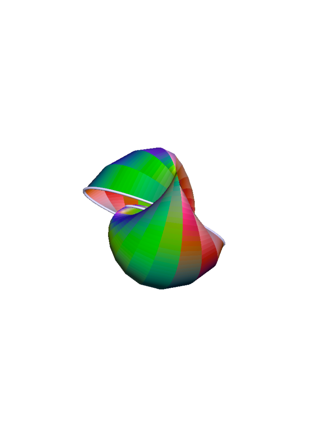
Figure 2: Surface corresponding to the first closed curve, partially cut to show the circles in grey, projected down to ℝ3{\mathbb{R}}^{3}.

First case: |C|>2|C|>2. Here the trajectories are bounded in the variable rr since

r=EC−2​sin⁡α.r=\sqrt{\frac{E}{C-2\sin\alpha}}.

therefore the curves γ\gamma are also bounded. In order to know whether such curves are closed, we calculate the variation of the angle of the curve with respect to the origin along a period of the variable α\alpha:

Φ⁡(C)=∫sin⁡αr​𝑑s=∫02​πsin⁡αC−2​sin⁡α​𝑑α.\Phi(C)=\int\frac{\sin\alpha}{r}ds=\int_{0}^{2\pi}\frac{\sin\alpha}{C-2\sin\alpha}d\alpha.

An easy computation shows that limC→±2=+∞\lim_{C\to\pm 2}=+\infty and limC→∞=0\lim_{C\to\infty}=0. It follows that for all rational numbers p/qp/q there exists C⁡(p/q)C(p/q) such that the corresponding curve Φ⁡(Cq)=2​p​π/q\Phi(C_{q})=2p\pi/q. By repeating qq times this pattern, we obtain a qq-symmetric curve. It is easy to check that these curves are never embedded.

Second case: |C|<2|C|<2. Here the trajectories are unbounded. However we still have

Φ⁡(C)=∫sin⁡αr​𝑑s=∫α−α+sin⁡αC−2​sin⁡α​𝑑α,\Phi(C)=\int\frac{\sin\alpha}{r}ds=\int_{\alpha_{-}}^{\alpha_{+}}\frac{\sin\alpha}{C-2\sin\alpha}d\alpha,

and

Φ⁡(C)=∫α+α−+2​πsin⁡αC−2​sin⁡α​𝑑α,\Phi(C)=\int_{\alpha_{+}}^{\alpha_{-}+2\pi}\frac{\sin\alpha}{C-2\sin\alpha}d\alpha,

where α−<α+\alpha_{-}<\alpha_{+} are defined to be the two roots of 2sinα±=C2\sin\alpha_{\pm}=C. In both cases, if CC does not vanish, Φ⁡(C)=∞\Phi(C)=\infty, therefore the curve γ\gamma has two ends which spiral. The case of vanishing CC implies β\beta to be constant, so this is the special Lagrangian case, which have already been treated in [A], Section 4 (cf also [CU]). It is proved that we get, up to congruences, a unique surface, the Lagrangian catenoid.

Third case: |C|=2|C|=2.

Here all the points of the vertical lines α=0modπ\alpha=0\bmod\pi are equilibrium points. The corresponding curves γ\gamma are round circles centered at the origin. The corresponding surfaces are products of circles 𝕊1​(r)×𝕊1​(r){\mathbb{S}}^{1}(r)\times{\mathbb{S}}^{1}(r), sometimes called Clifford tori. In the region α≠0modπ\alpha\neq 0\bmod\pi, the situation is analogous the second case: the curves γ\gamma have two spiraling ends.

4.2 Characterization of Hamiltonian stationary Type I surfaces

Proposition 2

A non-planar Hamiltonian stationary Lagrangian cyclic surface of ℂ2{\mathbb{C}}^{2} of type I must be centered, and thus is one of the surfaces described in Section 4.1

Proof. The proof is done by contradiction. We consider a type I immersion

Y:I×ℝ/2​π​ℤ→ℂ2(s,t)↦r⁡(s)​ei​ϕ​(s)​(cos⁡t,sin⁡t)+∫s0sei​ϕ​(u)​(W1​(u),W2​(u))​𝑑u\begin{array}[]{cccl}Y:&I\times\mathbb{R}/2\pi\mathbb{Z}&\to&\mathbb{C}^{2}\\ &(s,t)&\mapsto&r(s)e^{i\phi(s)}(\cos t,\sin t)+\int_{s_{0}}^{s}e^{i\phi(u)}(W_{1}(u),W_{2}(u))du\end{array}

with non-vanishing W=(W1,W2)W=(W_{1},W_{2}) and we show that the Hamiltonian stationarity leads to a contradiction. We recall some notations already introduced in [ACR]:

x=(cos⁡t,sin⁡t),x=(\cos t,\sin t),
A:=(1+⟨W,x⟩2+2cosα⟨W,x⟩)−1/2.A:=\left(1+\left\langle W,x\right\rangle^{2}+2\cos\alpha\langle W,x\rangle\right)^{-1/2}.

and

B:=k+(k​cos⁡α+sin⁡α​cos⁡αr)​⟨W,x⟩−sin⁡α⁡⟨W′,x⟩+sin⁡αr​⟨W,x⟩2.B:=k+\left(k\cos\alpha+\frac{\sin\alpha\cos\alpha}{r}\right)\left\langle W,x\right\rangle-\sin\alpha\left\langle W^{\prime},x\right\rangle+\frac{\sin\alpha}{r}\left\langle W,x\right\rangle^{2}.

We also exploit the computations done in [ACR], Section 4, where it was shown that

A−6​Δ​β=I+II+III+IV+V+VI+VIIA^{-6}\Delta\beta=\mathrm{I}+\mathrm{II}+\mathrm{III}+\mathrm{IV}+\mathrm{V}+\mathrm{VI}+\mathrm{VII}

where

I\displaystyle\mathrm{I} :⁣=\displaystyle:= 3​B​(cos⁡α⁡⟨W′,x⟩−α′​sin⁡α⁡⟨W,x⟩+⟨W,x⟩​⟨W′,x⟩)\displaystyle 3B\left(\cos\alpha\left\langle W^{\prime},x\right\rangle-\alpha^{\prime}\sin\alpha\left\langle W,x\right\rangle+\left\langle W,x\right\rangle\left\langle W^{\prime},x\right\rangle\right)
II\displaystyle\mathrm{II} :⁣=\displaystyle:= −A−2​[B′−sin⁡αr​(cos⁡α⁡⟨W′,x⟩−α′​sin⁡α⁡⟨W,x⟩+⟨W,x⟩​⟨W′,x⟩)]\displaystyle-A^{-2}\left[B^{\prime}-\frac{\sin\alpha}{r}\left(\cos\alpha\left\langle W^{\prime},x\right\rangle-\alpha^{\prime}\sin\alpha\left\langle W,x\right\rangle+\left\langle W,x\right\rangle\left\langle W^{\prime},x\right\rangle\right)\right]
III\displaystyle\mathrm{III} :⁣=\displaystyle:= −A−4∂s(sin⁡αr)\displaystyle-A^{-4}\partial_{s}\left(\frac{\sin\alpha}{r}\right)
IV\displaystyle\mathrm{IV} :⁣=\displaystyle:= −3​B​cos⁡α+⟨W,x⟩r​(|W|2−⟨W,x⟩2)\displaystyle-3B\frac{\cos\alpha+\left\langle W,x\right\rangle}{r}(|W|^{2}-\left\langle W,x\right\rangle^{2})
V\displaystyle\mathrm{V} :⁣=\displaystyle:= A−2r[(kcosα+sin⁡αr⟨W,x⟩)(|W|2−⟨W,x⟩2)\displaystyle\frac{A^{-2}}{r}\bigg[\left(k\cos\alpha+\frac{\sin\alpha}{r}\left\langle W,x\right\rangle\right)(|W|^{2}-\left\langle W,x\right\rangle^{2})
+sinα(⟨W′,W⟩−⟨W′,x⟩⟨W,x⟩)]\displaystyle+\sin\alpha\left(\left\langle W^{\prime},W\right\rangle-\left\langle W^{\prime},x\right\rangle\left\langle W,x\right\rangle\right)\bigg]
VI\displaystyle\mathrm{VI} :⁣=\displaystyle:= −A−2​sin⁡αr2​(cos⁡α+⟨W,x⟩)​(|W|2−⟨W,x⟩2)−2​A−4​sin⁡αr2​⟨W,x⟩\displaystyle-A^{-2}\frac{\sin\alpha}{r^{2}}(\cos\alpha+\left\langle W,x\right\rangle)\left(|W|^{2}-\left\langle W,x\right\rangle^{2}\right)-2A^{-4}\frac{\sin\alpha}{r^{2}}\left\langle W,x\right\rangle
VII\displaystyle\mathrm{VII} :⁣=\displaystyle:= −A−2​Br​(cos⁡α+⟨W,x⟩)−A−4​sin⁡α​cos⁡αr2\displaystyle-A^{-2}\frac{B}{r}(\cos\alpha+\left\langle W,x\right\rangle)-A^{-4}\frac{\sin\alpha\cos\alpha}{r^{2}}

For fixed ss we may view A−6​Δ​βA^{-6}\Delta\beta as a polynomial in xx; then the highest degree term is not anymore in ⟨W,x⟩5\left\langle W,x\right\rangle^{5} as in [ACR] but only in the fourth power. Forgetting all powers of xx beneath the fourth, we have:

I\displaystyle\mathrm{I} ≡\displaystyle\equiv 3​sin⁡αr​⟨W′,x⟩​⟨W,x⟩3\displaystyle\frac{3\sin\alpha}{r}\left\langle W^{\prime},x\right\rangle\left\langle W,x\right\rangle^{3}
II\displaystyle\mathrm{II} ≡\displaystyle\equiv −∂s(sin⁡αr)⟨W,x⟩4−sin⁡αr⟨W′,x⟩⟨W,x⟩3\displaystyle-\partial_{s}\left(\frac{\sin\alpha}{r}\right)\left\langle W,x\right\rangle^{4}-\frac{\sin\alpha}{r}\left\langle W^{\prime},x\right\rangle\left\langle W,x\right\rangle^{3}
III\displaystyle\mathrm{III} ≡\displaystyle\equiv −∂s(sin⁡αr)⟨W,x⟩4\displaystyle-\partial_{s}\left(\frac{\sin\alpha}{r}\right)\left\langle W,x\right\rangle^{4}
IV\displaystyle\mathrm{IV} ≡\displaystyle\equiv 3​sin⁡αr2​⟨W,x⟩5+(3​k​cos⁡αr+6​sin⁡α​cos⁡αr2)​⟨W,x⟩4\displaystyle\frac{3\sin\alpha}{r^{2}}\left\langle W,x\right\rangle^{5}+\left(\frac{3k\cos\alpha}{r}+\frac{6\sin\alpha\cos\alpha}{r^{2}}\right)\left\langle W,x\right\rangle^{4}
−3​sin⁡αr​⟨W′,x⟩​⟨W,x⟩3\displaystyle-\frac{3\sin\alpha}{r}\left\langle W^{\prime},x\right\rangle\left\langle W,x\right\rangle^{3}
V\displaystyle\mathrm{V} ≡\displaystyle\equiv −sin⁡αr2​⟨W,x⟩5−(k​cos⁡αr+2​sin⁡α​cos⁡αr2)​⟨W,x⟩4\displaystyle-\frac{\sin\alpha}{r^{2}}\left\langle W,x\right\rangle^{5}-\left(\frac{k\cos\alpha}{r}+\frac{2\sin\alpha\cos\alpha}{r^{2}}\right)\left\langle W,x\right\rangle^{4}
−sin⁡αr​⟨W′,x⟩​⟨W,x⟩3\displaystyle-\frac{\sin\alpha}{r}\left\langle W^{\prime},x\right\rangle\left\langle W,x\right\rangle^{3}
VI\displaystyle\mathrm{VI} ≡\displaystyle\equiv −sin⁡αr2​⟨W,x⟩5−5​sin⁡α​cos⁡αr2​⟨W,x⟩4\displaystyle-\frac{\sin\alpha}{r^{2}}\left\langle W,x\right\rangle^{5}-\frac{5\sin\alpha\cos\alpha}{r^{2}}\left\langle W,x\right\rangle^{4}
VII\displaystyle\mathrm{VII} ≡\displaystyle\equiv −sin⁡αr2​⟨W,x⟩5−(5​sin⁡α​cos⁡αr2+k​cos⁡αr)​⟨W,x⟩4\displaystyle-\frac{\sin\alpha}{r^{2}}\left\langle W,x\right\rangle^{5}-\left(\frac{5\sin\alpha\cos\alpha}{r^{2}}+\frac{k\cos\alpha}{r}\right)\left\langle W,x\right\rangle^{4}
+sin⁡αr​⟨W′,x⟩​⟨W,x⟩3\displaystyle+\frac{\sin\alpha}{r}\left\langle W^{\prime},x\right\rangle\left\langle W,x\right\rangle^{3}

At given ss, for Δ​β\Delta\beta to be zero for all tt, we need (replacing kk by α′+sin⁡α/r\alpha^{\prime}+\sin\alpha/r and using r′=cos⁡αr^{\prime}=\cos\alpha, ϕ′=sin⁡α/r\phi^{\prime}=\sin\alpha/r),

0\displaystyle 0 =\displaystyle= sin⁡αr​⟨W′,x⟩+(2​∂s(sin⁡αr)+5​sin⁡α​cos⁡αr2−α′​cos⁡αr)​⟨W,x⟩\displaystyle\frac{\sin\alpha}{r}\left\langle W^{\prime},x\right\rangle+\left(2\partial_{s}\left(\frac{\sin\alpha}{r}\right)+\frac{5\sin\alpha\cos\alpha}{r^{2}}-\frac{\alpha^{\prime}\cos\alpha}{r}\right)\left\langle W,x\right\rangle
=\displaystyle= sin⁡αr​⟨W′,x⟩+(∂s(sin⁡αr)+4​sin⁡α​cos⁡αr2)​⟨W,x⟩\displaystyle\frac{\sin\alpha}{r}\left\langle W^{\prime},x\right\rangle+\left(\partial_{s}\left(\frac{\sin\alpha}{r}\right)+\frac{4\sin\alpha\cos\alpha}{r^{2}}\right)\left\langle W,x\right\rangle

for almost all values, hence for all. If WW and W′W^{\prime} are not colinear, then ⟨W,x⟩\left\langle W,x\right\rangle and ⟨W′,x⟩\left\langle W^{\prime},x\right\rangle are linearly independent as functions of tt, hence

sin⁡αr=∂s(sin⁡αr)+4​sin⁡α​cos⁡αr2=0\frac{\sin\alpha}{r}=\partial_{s}\left(\frac{\sin\alpha}{r}\right)+\frac{4\sin\alpha\cos\alpha}{r^{2}}=0

so that θ≡ϕmodπ\theta\equiv\phi\bmod\pi, ϕ\phi is constant (and it is half the Lagrangian angle). The solution is then trivial: a subset of some Lagrangian plane, spanned by circles.

If W′W^{\prime} is colinear to WW for an open interval in the ss variable, then W⁡(s)=w⁡(s)​W0W(s)=w(s)W^{0} for some real valued function w⁡(s)w(s), and the center of the circle at ss lies in the plane ℂ​W0{\mathbb{C}}W^{0}. Using real rotations, and up to a reparametrization in tt, we may as well assume that W0=(1,0)W^{0}=(1,0) and we arrive at the following equation

sin⁡αr​w′+(∂s(sin⁡αr)+4​sin⁡α​cos⁡αr2)​w=0.\frac{\sin\alpha}{r}w^{\prime}+\left(\partial_{s}\left(\frac{\sin\alpha}{r}\right)+\frac{4\sin\alpha\cos\alpha}{r^{2}}\right)w=0.

whose solution (up to scaling) is w=c​(r3​sin⁡α)−1,w=c(r^{3}\sin\alpha)^{-1}, where cc is some non vanishing constant (the case of vanishing cc would correspond to the centered case). Using this last result, we shall now come back to the expression of A−6​Δ​βA^{-6}\Delta\beta. First, we have

A−2\displaystyle A^{-2} =\displaystyle= 1+2​w​cos⁡α​cos⁡t+w2​cos2⁡t\displaystyle 1+2w\cos\alpha\cos t+w^{2}\cos^{2}t
B\displaystyle B =\displaystyle= k+(k​cos⁡α+sin⁡α​cos⁡αr)​w​cos⁡t+cos⁡α⁡(k+2​sin⁡αr)​w​cos⁡t\displaystyle k+\left(k\cos\alpha+\frac{\sin\alpha\cos\alpha}{r}\right)w\cos t+\cos\alpha\left(k+\frac{2\sin\alpha}{r}\right)w\cos t
+sin⁡αr​w2​cos2⁡t\displaystyle+\frac{\sin\alpha}{r}w^{2}\cos^{2}t
=\displaystyle= k+(2​k​cos⁡α+3​sin⁡α​cos⁡αr)​w​cos⁡t+sin⁡αr​w2​cos2⁡t\displaystyle k+\left(2k\cos\alpha+\frac{3\sin\alpha\cos\alpha}{r}\right)w\cos t+\frac{\sin\alpha}{r}w^{2}\cos^{2}t
B′\displaystyle B^{\prime} =\displaystyle= k′+(2​k′​cos⁡α−2​k2sin⁡α−kr​(3​cos2⁡α+1)+sin⁡αr2​(3−15​cos2⁡α))​w​cos⁡t\displaystyle k^{\prime}+\left(2k^{\prime}\cos\alpha-\frac{2k^{2}}{\sin\alpha}-\frac{k}{r}(3\cos^{2}\alpha+1)+\frac{\sin\alpha}{r^{2}}(3-15\cos^{2}\alpha)\right)w\cos t
−(k​cos⁡αr+6​sin⁡α​cos⁡αr2)​w2​cos2⁡t\displaystyle-\left(\frac{k\cos\alpha}{r}+\frac{6\sin\alpha\cos\alpha}{r^{2}}\right)w^{2}\cos^{2}t

After a long but straightforward calculation, we get

A−6​Δ​β\displaystyle A^{-6}\Delta\beta =\displaystyle= −(k′+2​k​cos⁡αr+3​k​w2​cos⁡αr+3​w2​sin⁡α​cos⁡αr2−sin⁡α​cos⁡αr2)\displaystyle-\left(k^{\prime}+\frac{2k\cos\alpha}{r}+\frac{3kw^{2}\cos\alpha}{r}+\frac{3w^{2}\sin\alpha\cos\alpha}{r^{2}}-\frac{\sin\alpha\cos\alpha}{r^{2}}\right)
−(4​k′​cos⁡α+k2sin⁡α+k⁡(14​cos2⁡α−2)r−sin⁡αr2​(13​cos2⁡α−4)CLOSE\displaystyle-\left(4k^{\prime}\cos\alpha+\frac{k^{2}}{\sin\alpha}+\frac{k(14\cos^{2}\alpha-2)}{r}-\frac{\sin\alpha}{r^{2}}(13\cos^{2}\alpha-4)\right.
OPEN+k​w2r​(6​cos2⁡α+3)+w2​sin⁡α⁡(15​cos2⁡α)r2)​w​cos⁡t\displaystyle\hskip 10.00002pt\left.+\frac{kw^{2}}{r}(6\cos^{2}\alpha+3)+\frac{w^{2}\sin\alpha(15\cos^{2}\alpha)}{r^{2}}\right)w\cos t
−(k′​(1+4​cos2⁡α)+5​k2​cot⁡α+k​cos⁡αr​(20​cos2⁡α+13)CLOSE\displaystyle-\left(k^{\prime}(1+4\cos^{2}\alpha)+5k^{2}\cot\alpha+\frac{k\cos\alpha}{r}(20\cos^{2}\alpha+13)\right.
OPEN+sin⁡α​cos⁡αr2​(5​cos2⁡α−2)+6​k​cos⁡α​w2r+6​w2​sin⁡α​cos⁡αr2)​w2​cos2⁡t\displaystyle\quad\left.+\frac{\sin\alpha\cos\alpha}{r^{2}}(5\cos^{2}\alpha-2)+\frac{6k\cos\alpha w^{2}}{r}+\frac{6w^{2}\sin\alpha\cos\alpha}{r^{2}}\right)w^{2}\cos^{2}t
−(2​k′​cos⁡α+k2sin⁡α​(4​cos2⁡α)+kr​(22​cos2⁡α+1)CLOSE\displaystyle-\left(2k^{\prime}\cos\alpha+\frac{k^{2}}{\sin\alpha}(4\cos^{2}\alpha)+\frac{k}{r}(22\cos^{2}\alpha+1)\right.
OPEN+sin⁡αr2​(7​cos2⁡α+4+3​w2))​w3​cos3⁡t\displaystyle\quad\left.+\frac{\sin\alpha}{r^{2}}\left(7\cos^{2}\alpha+4+3w^{2}\right)\right)w^{3}\cos^{3}t

Thus the vanishing of Δ​β\Delta\beta implies four linear relations in the (dependent) variables k′​cos⁡αk^{\prime}\cos\alpha, k2/sin⁡αk^{2}/\sin\alpha, k/rk/r and sin⁡α/r2\sin\alpha/r^{2}, that we write in matrix form:

(10X⁡(2+3​w2)X⁡(3​w2−1)4114​X−2+(6​X+3)​w215​X​w2+4−13​X1+4​X5​XX⁡(20​X+13)+6​X​w2X⁡(6​w2+5​X−2)24​X22​X+13​w2+7​X+4)​(k′​cos⁡αk2/sin⁡αk/rsin⁡α/r2)=0\left(\begin{array}[]{cccc}1&0&X(2+3w^{2})&X(3w^{2}-1)\\ 4&1&14X-2+(6X+3)w^{2}&15Xw^{2}+4-13X\\ 1+4X&5X&X(20X+13)+6Xw^{2}&X(6w^{2}+5X-2)\\ 2&4X&22X+1&3w^{2}+7X+4\end{array}\right)\left(\begin{array}[]{c}k^{\prime}\cos\alpha\\ k^{2}/\sin\alpha\\ k/r\\ \sin\alpha/r^{2}\end{array}\right)=0

where we have denoted X=cos2⁡αX=\cos^{2}\alpha for brevity. We reduce it to

(10X⁡(2+3​w2)X⁡(3​w2−1)016​X−2+(−6​X+3)​w23​X​w2+4−9​X00X⁡(−18​X+21)+X⁡(18​X−12)​w2X⁡(3−27​X)​w2+X⁡(54​X−21)00−24​X2+26​X+1−X⁡(24​X−6)​w2w2​(3−6​X−12​X2)+4−7​X+36​X2)\left(\begin{array}[]{cccc}1&0&X(2+3w^{2})&X(3w^{2}-1)\\ 0&1&6X-2+(-6X+3)w^{2}&3Xw^{2}+4-9X\\ 0&0&X(-18X+21)+X(18X-12)w^{2}&X(3-27X)w^{2}+X(54X-21)\\ 0&0&-24X^{2}+26X+1-X(24X-6)w^{2}&w^{2}(3-6X-12X^{2})+4-7X+36X^{2}\end{array}\right) (2)

leaving us with the following system

{X⁡((−18​X+21)+(18​X−12)​w2)​k=X⁡((27​X−3)​w2+(21−54​X))​sin⁡αr(24​X2−26​X−1+X​w2​(24​X−6))​k=−(w2​(3−6​X−12​X2)+4−7​X+36​X2)​sin⁡αr\left\{\begin{array}[]{l}X((-18X+21)+(18X-12)w^{2})k\\ \hskip 85.35826pt=X((27X-3)w^{2}+(21-54X))\frac{\sin\alpha}{r}\\ (24X^{2}-26X-1+Xw^{2}(24X-6))k\\ \hskip 85.35826pt=-(w^{2}(3-6X-12X^{2})+4-7X+36X^{2})\frac{\sin\alpha}{r}\end{array}\right. (3)

The trivial solution k=sin⁡α=0k=\sin\alpha=0 being excluded because ww is not defined when sin⁡α=0\sin\alpha=0, the determinant of the above system must vanish, hence the following algebraic equation

E⁡(X,Y)=(−288​X3+90​X2+36​X−12)​Y2+(−504​X4+756​X3−264​X2+8​X+4)​Y+216​X5−774​X4+991​X3−489​X2+21​X+35E(X,Y)=\left(-288X^{3}+90X^{2}+36X-12\right)Y^{2}\\ +\left(-504X^{4}+756X^{3}-264X^{2}+8X+4\right)Y\\ +216X^{5}-774X^{4}+991X^{3}-489X^{2}+21X+35 (4)

in terms of the variables X=cos2⁡αX=\cos^{2}\alpha and Y=c2​r−6=w2​sin2⁡αY=c^{2}r^{-6}=w^{2}\sin^{2}\alpha, where we have divided by XX for simplicity. We will now show a contradiction. Indeed any of the two equations in (3) yields a dynamical system

{α′=k−sin⁡αr=sin⁡αr​g​(cos2⁡α,c2​r−6)r′=cos⁡α\left\{\begin{array}[]{l}\alpha^{\prime}=k-\frac{\sin\alpha}{r}=\frac{\sin\alpha}{r}g(\cos^{2}\alpha,c^{2}r^{-6})\\ r^{\prime}=\cos\alpha\end{array}\right.

and if we take for instance the first one

g⁡(X,Y)=(5+19​X+12​X2)​(1−X)+Y⁡(3−36​X)(24​X2−26​X−1)​(1−X)+Y⁡(24​X2−6​X).g(X,Y)=\frac{(5+19X+12X^{2})(1-X)+Y(3-36X)}{(24X^{2}-26X-1)(1-X)+Y(24X^{2}-6X)}.

The solution (α⁡(s),r⁡(s))(\alpha(s),r(s)) has to satisfy the analytic equation E⁡(cos2⁡α,c2​r−6)=0E(\cos^{2}\alpha,c^{2}r^{-6})=0. Taking the derivative leads to

2​sin⁡α​cos⁡α​α′​∂E/∂X+6​c2​r′​r−7​∂E/∂Y=0,2\sin\alpha\cos\alpha\alpha^{\prime}\partial E/\partial X+6c^{2}r^{\prime}r^{-7}\partial E/\partial Y=0,

which expands to

F⁡(X,Y):=(1−X)​g​(X,Y)​∂E∂X+3​Y​∂E∂Y=0.F(X,Y):=(1-X)g(X,Y)\frac{\partial E}{\partial X}+3Y\frac{\partial E}{\partial Y}=0\,.

For a solution to exist, we need to find a common open set for the two algebraic curves E=0E=0 and F=0F=0. However EE is irreducible, so if EE and FF agree, they have to do so on the complete component E=0E=0. We show on the contrary that this component contains a point that does not satisfy F=0F=0. Let us solve E⁡(0,Y)=0E(0,Y)=0.

0=E⁡(0,Y)=−12​Y2+4​Y+350=E(0,Y)=-12Y^{2}+4Y+35

yields Y=1±1066Y=\frac{1\pm\sqrt{106}}{6}. Evaluating FF at these two values yields 1100±85​1061100\pm 85\sqrt{106} which are non zero, hence the contradiction. Finally we study the case of X=cos2⁡α=0X=\cos^{2}\alpha=0, where the system (2) amounts to

{k2sin⁡α−2​kr+3​k​w2r+4​sin⁡αr2=0kr+3​w2​sin⁡αr2+4​sin⁡αr2​0\left\{\begin{array}[]{l}\displaystyle\frac{k^{2}}{\sin\alpha}-\frac{2k}{r}+\frac{3kw^{2}}{r}+\frac{4\sin\alpha}{r^{2}}=0\\ \displaystyle\frac{k}{r}+\frac{3w^{2}\sin\alpha}{r^{2}}+\frac{4\sin\alpha}{r^{2}}0\end{array}\right.

and since k=α′+sin⁡α/r=sin⁡α/rk=\alpha^{\prime}+\sin\alpha/r=\sin\alpha/r

{sin⁡αr2−2​sin⁡αr2+3​sin⁡α​w2r2+4​sin⁡αr2=0sin⁡αr2+3​w2​sin⁡αr2+4​sin⁡αr2=0\left\{\begin{array}[]{l}\displaystyle\frac{\sin\alpha}{r^{2}}-\frac{2\sin\alpha}{r^{2}}+\frac{3\sin\alpha w^{2}}{r^{2}}+\frac{4\sin\alpha}{r^{2}}=0\\ \displaystyle\frac{\sin\alpha}{r^{2}}+\frac{3w^{2}\sin\alpha}{r^{2}}+\frac{4\sin\alpha}{r^{2}}=0\end{array}\right.
3+3​w2=5+3​w2=03+3w^{2}=5+3w^{2}=0

so again we get a contradiction and the proof is complete.

4.3 Hamiltonian stationary Type II surfaces

Proposition 3

A Hamiltonian stationary Lagrangian cyclic surface of ℂ2{\mathbb{C}}^{2} of type II is locally congruent to a Cartesian product of two round circles 𝕊1​(r1)×𝕊1​(r2){\mathbb{S}}^{1}(r_{1})\times{\mathbb{S}}^{1}(r_{2}).

Proof. As we saw in Section 2, Remark 4, a type II immersion which is not a product of curves can take the following form

X:I×ℝ/2​π​ℤ→ℂ2(s,t)↦c⁡(γ1​(s)​ei​t,γ2​(s)​ei​t)+∫s0sW⁡(u)​(γ1′,γ2′)​𝑑u\begin{array}[]{clcl}X:&I\times{\mathbb{R}}/2\pi{\mathbb{Z}}&\to&{\mathbb{C}}^{2}\\ &(s,t)&\mapsto&c(\gamma_{1}(s)e^{it},\gamma_{2}(s)e^{it})+\int_{s_{0}}^{s}W(u)(\gamma^{\prime}_{1},\gamma^{\prime}_{2})du\end{array}

where the Legendrian curve γ=(γ1,γ2)\gamma=(\gamma_{1},\gamma_{2}) is parametrized by arc length. We denote by βL=arg⁡(γ1​γ2′−γ2​γ1′)\beta_{L}=\arg(\gamma_{1}\gamma^{\prime}_{2}-\gamma_{2}\gamma^{\prime}_{1}) the Legendrian angle of the curve γ=(γ1,γ2)\gamma=(\gamma_{1},\gamma_{2}), i.e. the Lagrangian angle of the plane spanned by γ,γ′\gamma,\gamma^{\prime}. Next we compute the derivatives of the immersion (we set the constant cc to 11 since that does not change the Lagrangian angle):

Ys=(W+ei​t)​(γ1′γ2′),Yt=i​ei​t​(γ1γ2),Y_{s}=(W+e^{it})\left(\begin{array}[]{c}\gamma^{\prime}_{1}\\ \gamma^{\prime}_{2}\end{array}\right)\;,\hskip 10.00002ptY_{t}=ie^{it}\left(\begin{array}[]{c}\gamma_{1}\\ \gamma_{2}\end{array}\right),

from which we deduce that

detℂ(Ys,Yt)=i​ei​t​(W+ei​t)​(γ1′​γ2−γ2′​γ1)=−i⁡(ei​t+W)​ei⁡(βL+t){\det}_{{\mathbb{C}}}(Y_{s},Y_{t})=ie^{it}(W+e^{it})(\gamma^{\prime}_{1}\gamma_{2}-\gamma^{\prime}_{2}\gamma_{1})=-i(e^{it}+W)e^{i(\beta_{L}+t)}

Thus

β⁡(s,t)=t+βL+arctan⁡(sin⁡t+W2cos⁡t+W1)−π2\beta(s,t)=t+\beta_{L}+\arctan\left(\frac{\sin t+W_{2}}{\cos t+W_{1}}\right)-\frac{\pi}{2}

We now compute the induced metric:

gs​s=1+|W|2+2​⟨W,ei​t⟩=:A2gt​t=1gs​t=0,g_{ss}=1+|W|^{2}+2\langle W,e^{it}\rangle=:A^{2}\quad g_{tt}=1\quad g_{st}=0,

and the first derivatives of β:\beta:

βs=βL′+⟨W′,i​ei​t⟩+W1​W2′−W1′​W2A2,βt=2+|W|2+3​⟨W,ei​t⟩A2,\beta_{s}=\beta^{\prime}_{L}+\frac{\langle W^{\prime},ie^{it}\rangle+W_{1}W^{\prime}_{2}-W^{\prime}_{1}W_{2}}{A^{2}}\;,\hskip 10.00002pt\beta_{t}=\frac{2+|W|^{2}+3\langle W,e^{it}\rangle}{A^{2}}\;,

where ⟨,⟩\left\langle,\right\rangle stands for the scalar product in ℂ≃ℝ2{\mathbb{C}}\simeq{\mathbb{R}}^{2}.

g=(A2001),g−1=(A−2001).g=\left(\begin{array}[]{cc}A^{2}&0\\ 0&1\end{array}\right),\hskip 10.00002ptg^{-1}=\left(\begin{array}[]{cc}A^{-2}&0\\ 0&1\end{array}\right)\;.

Thus,

Δ​β=−1detg​(∂∂s​(detg​gs​s​βs)+∂∂t​(detg​gt​t​βt))\Delta\beta=-\frac{1}{\sqrt{\det g}}\left(\frac{\partial}{\partial s}\left(\sqrt{\det g}g^{ss}\beta_{s}\right)+\frac{\partial}{\partial t}\left(\sqrt{\det g}g^{tt}\beta_{t}\right)\right)
−A​Δ​β\displaystyle-A\Delta\beta =\displaystyle= ∂∂s​(1A​(βL′+⟨W′,i​ei​t⟩+W1​W2′−W1′​W2A2))\displaystyle\frac{\partial}{\partial s}\left(\frac{1}{A}\left(\beta^{\prime}_{L}+\frac{\langle W^{\prime},ie^{it}\rangle+W_{1}W^{\prime}_{2}-W^{\prime}_{1}W_{2}}{A^{2}}\right)\right)
+∂∂t​(2+|W|2+3​⟨W,ei​t⟩A)\displaystyle+\frac{\partial}{\partial t}\left(\frac{2+|W|^{2}+3\langle W,e^{it}\rangle}{A}\right)
=\displaystyle= βL′′​A−βL′​∂A∂sA2+⟨W′′,i​ei​t⟩+W1​W2′′−W1′′​W2A3\displaystyle\frac{\beta^{\prime\prime}_{L}A-\beta_{L}^{\prime}\frac{\partial A}{\partial s}}{A^{2}}+\frac{\left\langle W^{\prime\prime},ie^{it}\right\rangle+W_{1}W^{\prime\prime}_{2}-W^{\prime\prime}_{1}W_{2}}{A^{3}}
−3​⟨W′,i​ei​t⟩+W1​W2′−W1′​W2A4​∂A∂s\displaystyle-3\frac{\langle W^{\prime},ie^{it}\rangle+W_{1}W^{\prime}_{2}-W^{\prime}_{1}W_{2}}{A^{4}}\frac{\partial A}{\partial s}
+3​⟨W,i​ei​t⟩A−2+|W|2+3​⟨W,ei​t⟩A2​∂A∂t\displaystyle+3\frac{\left\langle W,ie^{it}\right\rangle}{A}-\frac{2+|W|^{2}+3\langle W,e^{it}\rangle}{A^{2}}\frac{\partial A}{\partial t}
=\displaystyle= βL′′A−βL′​⟨W′,W+ei​t⟩A3+⟨W′′,i​ei​t⟩+W1​W2′′−W1′′​W2A3\displaystyle\frac{\beta^{\prime\prime}_{L}}{A}-\frac{\beta_{L}^{\prime}\left\langle W^{\prime},W+e^{it}\right\rangle}{A^{3}}+\frac{\left\langle W^{\prime\prime},ie^{it}\right\rangle+W_{1}W^{\prime\prime}_{2}-W^{\prime\prime}_{1}W_{2}}{A^{3}}
−3​(⟨W′,i​ei​t⟩+W1​W2′−W1′​W2)​⟨W′,W+ei​t⟩A5\displaystyle-3\frac{\left(\langle W^{\prime},ie^{it}\rangle+W_{1}W^{\prime}_{2}-W^{\prime}_{1}W_{2}\right)\left\langle W^{\prime},W+e^{it}\right\rangle}{A^{5}}
+3​⟨W,i​ei​t⟩A−2+|W|2+3​⟨W,ei​t⟩A3​⟨W,i​ei​t⟩\displaystyle+3\frac{\left\langle W,ie^{it}\right\rangle}{A}-\frac{2+|W|^{2}+3\langle W,e^{it}\rangle}{A^{3}}\left\langle W,ie^{it}\right\rangle
−A6​Δ​β\displaystyle-A^{6}\Delta\beta =\displaystyle= A4​βL′′−A2​βL′​⟨W′,W+ei​t⟩+A2​(⟨W′′,i​ei​t⟩+W1​W2′′−W1′′​W2)\displaystyle A^{4}\beta^{\prime\prime}_{L}-A^{2}\beta_{L}^{\prime}\left\langle W^{\prime},W+e^{it}\right\rangle+A^{2}(\left\langle W^{\prime\prime},ie^{it}\right\rangle+W_{1}W^{\prime\prime}_{2}-W^{\prime\prime}_{1}W_{2})
−3​(⟨W′,i​ei​t⟩+W1​W2′−W1′​W2)​⟨W′,W+ei​t⟩\displaystyle-3\left(\langle W^{\prime},ie^{it}\rangle+W_{1}W^{\prime}_{2}-W^{\prime}_{1}W_{2}\right)\left\langle W^{\prime},W+e^{it}\right\rangle
+A2​⟨W,i​ei​t⟩​(1+2​|W|2+3​⟨W,ei​t⟩).\displaystyle+A^{2}\left\langle W,ie^{it}\right\rangle\left(1+2|W|^{2}+3\left\langle W,e^{it}\right\rangle\right).

For fixed ss, the expression −A6​Δ​β-A^{6}\Delta\beta is polynomial of degree 3 in the variable ei​te^{it}, and the only term of order 3 comes from the last line in the expression above: 3​A2​⟨W,ei​t⟩​⟨W,i​ei​t⟩3A^{2}\left\langle W,e^{it}\right\rangle\left\langle W,ie^{it}\right\rangle. Thus if β\beta is harmonic WW must vanish, hence we are in the centered case (Hopf type tori).

This case is straightforward: on the one hand the metric is flat and on the other hand β=2​t+βL−π2\beta=2t+\beta_{L}-\frac{\pi}{2}, thus we must have βL′′=0\beta^{\prime\prime}_{L}=0. Following the terminology of [CLU], the curve γ\gamma is contact stationary and take the following form :

γ(s)=(cei​s/2​c,1−c2e−is/2​(1−c2)),\gamma(s)=(ce^{is/\sqrt{2}c},\sqrt{1-c^{2}}e^{-is/\sqrt{2(1-c^{2})}}),

where c∈(0,1)c\in(0,1). We observe that the closedness of the Legendrian curve is not necessary in order to get a compact surface. The corresponding Hopf torus is a product of circles 𝕊1​(c)×𝕊1​(1−c2){\mathbb{S}}^{1}(c)\times{\mathbb{S}}^{1}(\sqrt{1-c^{2}}). By making a convenient homothety we get any product of circles 𝕊1​(r1)×𝕊1​(r2){\mathbb{S}}^{1}(r_{1})\times{\mathbb{S}}^{1}(r_{2}) thus the proof is complete.

5 Ruled Lagrangian surfaces

Let Σ\Sigma be a smooth, ruled, Lagrangian surface. If the rulings are parallel, it is straightforward that Σ\Sigma is a Cartesian product ℒ×Γ{\cal L}\times{\Gamma} of some straight line ℒ{\cal L}, and some planar curve Γ\Gamma, such that ℒ⊂P1{\cal L}\subset P_{1} and Γ⊂P2{\Gamma}\subset P_{2}, where P1P_{1} and P2P_{2} are two orthogonal, complex planes. So from now on, our discussion being local, we shall assume that the rulings are not parallel.

Locally, Σ\Sigma may be parametrized by the following immersion:

X:I×ℝ→ℂ2(s,t)↦γ⁡(s)​t+V⁡(s),\begin{array}[]{clcl}X:&I\times{\mathbb{R}}&\to&{\mathbb{C}}^{2}\\ &(s,t)&\mapsto&\gamma(s)t+V(s),\end{array}

where γ⁡(s)\gamma(s) is a unit speed curve of 𝕊3{\mathbb{S}}^{3} and V⁡(s)∈ℂ2V(s)\in{\mathbb{C}}^{2}, and we have

Xs=γ′​t+V′,Xt=γ.X_{s}=\gamma^{\prime}t+V^{\prime},\hskip 30.00005ptX_{t}=\gamma.

We now claim that, without loss of generality, we may assume that XsX_{s} and XtX_{t} are orthogonal: to see this, we reparametrize the surface by X^​(s,t)=X⁡(s,t)+γ⁡(s)​T​(s)\hat{X}(s,t)=X(s,t)+\gamma(s)T(s), where T⁡(s)T(s) is some real function. We observe that the images of XX and X^\hat{X} are the same. Then we compute

X^s=Xs+γ′​T+γ​T′,X^t=Xt=γ.\hat{X}_{s}=X_{s}+\gamma^{\prime}T+\gamma T^{\prime},\hskip 30.00005pt\hat{X}_{t}=X_{t}=\gamma.

Thus by choosing TT such that T′=−⟨Xs,Xt⟩T^{\prime}=-\langle X_{s},X_{t}\rangle, we may reparametrize our surface such that X^s\hat{X}_{s} and X^t\hat{X}_{t} are orthogonal.

The Lagrangian assumption amounts to

ω⁡(Xs,Xt)=⟨Xs,J​Xt⟩=t⁡⟨γ′,J​γ⟩+⟨V′,J​γ⟩=0.\omega(X_{s},X_{t})=\langle X_{s},JX_{t}\rangle=t\langle\gamma^{\prime},J\gamma\rangle+\langle V^{\prime},J\gamma\rangle=0.

The vanishing of ⟨γ′,J​γ⟩\langle\gamma^{\prime},J\gamma\rangle means that the curve γ\gamma is Legendrian. It follows that (γ,J​γ,γ′,J​γ′)(\gamma,J\gamma,\gamma^{\prime},J\gamma^{\prime}) is an orthonormal basis of ℝ4≃ℂ2{\mathbb{R}}^{4}\simeq{\mathbb{C}}^{2}. Thus the conditions ⟨V′,J​γ⟩=0\langle V^{\prime},J\gamma\rangle=0 and ⟨Xs,Xt⟩=⟨V′,γ⟩=0\langle X_{s},X_{t}\rangle=\langle V^{\prime},\gamma\rangle=0 imply that there exists a planar curve α⁡(s)=x⁡(s)+i​y​(s)\alpha(s)=x(s)+iy(s) such that V′=x​γ′+y​J​γ′=α​γ′V^{\prime}=x\gamma^{\prime}+yJ\gamma^{\prime}=\alpha\gamma^{\prime}. So we have shown the first part of the following:

Theorem 4

A smooth, ruled, Lagrangian surface of ℂ2{\mathbb{C}}^{2} is either the Cartesian product ℒ×Γ\mathcal{L}\times\Gamma of a straight line ℒ\mathcal{L} with a planar curve Γ\Gamma or may be locally parametrized by an immersion of the form

X:I×ℝ→ℂ2(s,t)↦γ⁡(s)​t+∫s0sα⁡(u)​(γ1′​(u),γ2′​(u))​du,\begin{array}[]{clcl}X:&I\times{\mathbb{R}}&\to&{\mathbb{C}}^{2}\\ &(s,t)&\mapsto&\gamma(s)t+\int_{s_{0}}^{s}\alpha(u)(\gamma_{1}^{\prime}(u),\gamma_{2}^{\prime}(u))du,\end{array}

where γ=(γ1,γ2)\gamma=(\gamma_{1},\gamma_{2}) is some Legendrian curve of 𝕊3{\mathbb{S}}^{3} and α=(x,y)\alpha=(x,y) is some planar curve. Moreover, the only self-similar ruled Lagrangian surfaces of ℂ2{\mathbb{C}}^{2} are Cartesian products ℒ×Γ\mathcal{L}\times\Gamma, where ℒ\mathcal{L} is a straight line and Γ{\Gamma} is a planar self-similar curve (cf [AL]).

Proof. We have already characterized ruled Lagrangian surfaces, so it remains to study the self-similar equation.

We start computing the first derivatives of the immersion:

Xt​(s,t)=γ⁡(s),Xs​(s,t)=(1+α⁡(s))​(γ1′​(s),γ2′​(s))X_{t}(s,t)=\gamma(s),\hskip 30.00005ptX_{s}(s,t)=(1+\alpha(s))(\gamma^{\prime}_{1}(s),\gamma^{\prime}_{2}(s))

from which we deduce the expression of the induced metric:

E=(t+x)2+y2,G=1,F=0,E=(t+x)^{2}+y^{2},\hskip 30.00005ptG=1,\hskip 30.00005ptF=0,

and a basis of the normal bundle:

Nt=i​γ​(s),Ns=i⁡(1+α⁡(s))​(γ1′​(s),γ2′​(s)).N_{t}=i\gamma(s),\hskip 30.00005ptN_{s}=i(1+\alpha(s))(\gamma^{\prime}_{1}(s),\gamma^{\prime}_{2}(s)).

We now compute some second derivatives:

Xs​t=γ′​(s),Xt​t=0.X_{st}=\gamma^{\prime}(s),\hskip 30.00005ptX_{tt}=0.

We deduce that

2​⟨H,Nt⟩=⟨Xs​s,Nt⟩E+⟨Xt​t,Nt⟩G=⟨Xs​t,Ns⟩E=1+x(t+x)2+y2.2\langle H,N_{t}\rangle=\frac{\langle X_{ss},N_{t}\rangle}{E}+\frac{\langle X_{tt},N_{t}\rangle}{G}=\frac{\langle X_{st},N_{s}\rangle}{E}=\frac{1+x}{(t+x)^{2}+y^{2}}.

On another hand, we have:

⟨X,Nt⟩=⟨i​γ​(s),∫s0sα⁡(u)​(γ1′​(u),γ2′​(u))​𝑑u⟩,\langle X,N_{t}\rangle=\langle i\gamma(s),\int_{s_{0}}^{s}\alpha(u)(\gamma_{1}^{\prime}(u),\gamma_{2}^{\prime}(u))du\rangle,

which clearly does not depend on tt. So the equation

⟨H,Nt⟩+λ⁡⟨X,Nt⟩=0\langle H,N_{t}\rangle+\lambda\langle X,N_{t}\rangle=0

can never hold for such an immersion, so the only self-similar ruled Lagrangian surfaces are products ℒ×Γ{\cal L}\times{\Gamma}. It is then straightforward to see that the curve Γ{\Gamma} must be a solution of the self-similar equation.

Remark 5

We recover the Lagrangian helicoid of [B] by taking γ⁡(s)=(k+i​l)​(cos⁡s,sin⁡s)\gamma(s)=(k+il)(\cos s,\sin s), where kk and ll are two constants such that k2+l2=1k^{2}+l^{2}=1. In the notation of [B], we have x⁡(s)=G/2x(s)=G/2 and y⁡(s)=−Ay(s)=-A.

References

  • [AL] U. Abresch, J. Langer, The normalized curve shortening flow and homothetic solutions, J. of Diff. Geom. 23 (1986), 175–196.
  • [ACR] H. Anciaux, I. Castro, P. Romon, Lagrangian submanifolds of ℝ2​n{\mathbb{R}}^{2n} which are foliated by spheres, Acta Math. Sinica (English Series), 22 (2006) no. 4, 1197–1214.
  • [A] H. Anciaux, Construction of Lagrangian self-similar solutions to the Mean Curvature Flow in ℂn{\mathbb{C}}^{n}, Geometriae Dedicata 120 (2006), 37–48.
  • [B] D. Blair, Lagrangian helicoids, Michigan Math. J. 50 (2002), no. 1, 187–200.
  • [CC] I. Castro, B.-Y. Chen, Lagrangian surfaces in complex Euclidean plane via spherical and hyperbolic curves, to appear in Tohoku Math. J. 58 (2006), no. 4.
  • [CLU] I. Castro, H. Li, F. Urbano, Hamiltonian-minimal Lagrangian submanifolds in complex space forms, Pacific J. of Maths. 227 (2006), no. 1, 43–61.
  • [CU] I. Castro, F. Urbano, On a Minimal Lagrangian Submanifold of ℂn{\mathbb{C}}^{n} Foliated by Spheres, Mich. Math. J. 46 (1999), 71–82
  • [C1] B.-Y. Chen, Complex extensors and Lagrangian submanifolds in complex Euclidean spaces, Tohoku Math. J. (2) 49 (1997), 277–297.
  • [C2] B.-Y. Chen, Construction of Lagrangian surfaces in complex Euclidean plane with Legendre curves, Kodai Math. J., 29 (2006), 84–112.
  • [HR] F. Hélein, P. Romon, Hamiltonian stationary Lagrangian surfaces in ℂ2{\mathbb{C}}^{2}, Comm. Anal. Geom. 10 (2002), 79–126.
  • [P] U. Pinkall, Hopf tori in 𝕊3{\mathbb{S}}^{3}, Invent. Math. 81 (1985), no. 2, 379–386.

Henri Anciaux
Departement of Mathematics and Computing
Institute of Technology, Tralee
Co. Kerry, Ireland
henri.anciaux@staff.ittralee.ie

Pascal Romon
Université de Paris-Est Marne-la-Vallée
5, bd Descartes, Champs-sur-Marne
77454 Marne-la-Vallée cedex 2, France
pascal.romon@univ-mlv.fr