An infinite presentation of the Torelli group

Andrew Putman

Abstract

In this paper, we construct an infinite presentation of the Torelli subgroup of the mapping class group of a surface whose generators consist of the set of all “separating twists”, all “bounding pair maps”, and all “commutators of simply intersecting pairs” and whose relations all come from a short list of topological configurations of these generators on the surface. Aside from a few obvious ones, all of these relations come from a set of embeddings of groups derived from surface groups into the Torelli group. In the process of analyzing these embeddings, we derive a novel presentation for the fundamental group of a closed surface whose generating set is the set of all simple closed curves.

1 Introduction

Let $\Sigma_{g}$ be a closed genus $g$ surface and $\Mod_{g}$ be the mapping class group of $\Sigma_{g}$ , that is, the group of homotopy classes of orientation-preserving diffeomorphisms of $\Sigma_{g}$ . The action of $\Mod_{g}$ on $\HH_{1}(\Sigma_{g};\text{$\mathbb{Z}$})$ preserves the algebraic intersection form, so it induces a representation $\Mod_{g}\rightarrow\Sp_{2g}(\text{$\mathbb{Z}$})$ . The kernel $\text{${\mathcal{I}}$}_{g}$ of this representation is known as the Torelli group. It plays an important role in both low-dimensional topology and algebraic geometry. See [16] for a survey of $\text{${\mathcal{I}}$}_{g}$ , especially the remarkable work of Dennis Johnson.

Despite the Torelli group’s importance, little is known about its combinatorial group theory. Generators for $\text{${\mathcal{I}}$}_{g}$ were first found by Birman and Powell [3, 28] (see below). Later, Johnson [17] constructed a finite generating set for $\text{${\mathcal{I}}$}_{g}$ for $g\geq 3$ , while McCullough and Miller [24] proved that $\text{${\mathcal{I}}$}_{2}$ is not finitely generated. The investigation of the genus $2$ case was completed by Mess [25], who proved that $\text{${\mathcal{I}}$}_{2}$ is an infinitely generated free group, though no explicit free generating set is known. However, the basic question of whether $\text{${\mathcal{I}}$}_{g}$ is ever finitely presented for $g\geq 3$ remains open.

In this paper, we construct an infinite presentation for $\text{${\mathcal{I}}$}_{g}$ whose generators and relations have simple topological interpretations. This is not the first presentation of the Torelli group in the literature – another appears in a paper of Morita and Penner [26]. However, while their generators and relations have nice interpretations in terms of a certain triangulation of Teichmüller space, they are topologically and group-theoretically extremely complicated. Indeed, their generating set contains infinitely many copies of every element of the Torelli group. Our methods and perspective are very different from theirs.

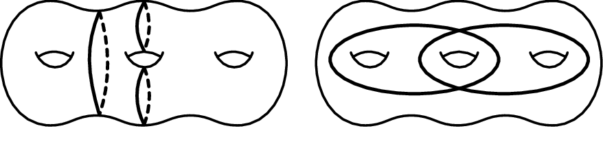
Refer to caption — Figure 1: a. A separating curve $x_{1}$ and a bounding pair $\{x_{2},x_{3}\}$ b. A simply intersecting pair $\{x_{4},x_{5}\}$

Generators.

Letting $T_{\gamma}$ be the right Dehn twist about a simple closed curve $\gamma$ , our generators are all mapping classes of the following types.

1.

Let $\gamma$ be a simple closed curve that separates the surface (for instance, the curve $x_{1}$ in Figure 1.a). Then it is not hard to see that $T_{\gamma}\in\text{${\mathcal{I}}$}_{g}$ . These are known as separating twists.
2.

Let $\{\gamma_{1},\gamma_{2}\}$ be a pair of non-isotopic disjoint homologous curves (for instance, the pair of curves $\{x_{2},x_{3}\}$ from Figure 1.a). Then $T_{\gamma_{1}}$ and $T_{\gamma_{2}}$ map to the same element of $\Sp_{2g}(\text{$\mathbb{Z}$})$ , so $T_{\gamma_{1}}T_{\gamma_{2}}^{-1}\in\text{${\mathcal{I}}$}_{g}$ . These are known as bounding pair maps. We will denote them by $T_{\gamma_{1},\gamma_{2}}$ .
3.

Let $\{\gamma_{1},\gamma_{2}\}$ be a pair of curves whose algebraic intersection number is $0$ . Then the images of $T_{\gamma_{1}}$ and $T_{\gamma_{2}}$ in $\Sp_{2g}(\text{$\mathbb{Z}$})$ commute, so $[T_{\gamma_{1}},T_{\gamma_{2}}]\in\text{${\mathcal{I}}$}_{g}$ . We will make use of such commutators for simple closed curves $\gamma_{1}$ and $\gamma_{2}$ whose geometric intersection number is $2$ (for instance, the pair of curves $\{x_{4},x_{5}\}$ from Figure 1.b). We will call these commutators of simply intersecting pairs and denote them by $C_{\gamma_{1},\gamma_{2}}$ .

Remarks.

•

The fact that $\text{${\mathcal{I}}$}_{g}$ is generated by separating twists and bounding pair maps follows from work of Birman and Powell ([3, 28]; see also [29] for a different proof, as well as generalizations)
•

Warning : Traditionally, the curves in a bounding pair are required to be nonseparating; however, to simplify our statements we allow them to be separating.
•

Commutators of simply intersecting pairs are not needed to generate $\text{${\mathcal{I}}$}_{g}$ , but their presence greatly simplifies our relations. We remark that the expression of a mapping class as a commutator of a simply intersecting pair is not unique; see Example 3.1 for an example.

Relations.

Our relations are as follows; a more detailed description follows.

1.

The formal relations (F.1)-(F.8). An example is $T_{\gamma_{1},\gamma_{2}}=T_{\gamma_{2},\gamma_{1}}^{-1}$ .
2.

Two families of relations (the lantern relations and the crossed lantern relations) that arise from easy identities among various ways of “dragging subsurfaces around”.
3.

Two families of relations (the Witt–Hall relations and the commutator shuffle relations) that arise from easy identities among various ways of “dragging bases of handles around”.

Formal relations.

These relations are formal in the sense that they are either immediate consequences of the standard expressions of our generators as products of Dehn twists or are consequences of the conjugation relation $fT_{x}f^{-1}=T_{f(x)}$ , where $x$ is a simple closed curve and $f$ is a mapping class. The first three are immediate, and are true for any curves $x_{1}$ , $x_{2}$ , and $x_{3}$ so that the expressions make sense.

$\displaystyle T_{x_{1},x_{2}}$	$\displaystyle=T_{x_{2},x_{1}}^{-1},$	(F.1)
$\displaystyle C_{x_{1},x_{2}}$	$\displaystyle=C_{x_{2},x_{1}}^{-1},$	(F.2)
$\displaystyle T_{x_{1},x_{2}}T_{x_{2},x_{3}}$	$\displaystyle=T_{x_{1},x_{3}}.$	(F.3)

Next, if $\{x_{1},x_{2}\}$ is a bounding pair so that both $x_{1}$ and $x_{2}$ are separating curves, we need

T_{x_{1},x_{2}}=T_{x_{1}}T_{x_{2}}^{-1}.\\

(F.4)

If $\{x_{1},x_{2}\}$ is a bounding pair and $\{x_{3},x_{2}\}$ is a simply intersecting pair so that $x_{1}$ and $x_{3}$ are disjoint, we need

T_{x_{1},T_{x_{3}}^{-1}(x_{2})}=C_{x_{3},x_{2}}T_{x_{1},x_{2}}.\\

(F.5)

Finally, we will also need the following conjugation relations. In them, $A$ is any generator and $x$ , $x_{1}$ , and $x_{2}$ are any curves so that the expressions make sense.

$\displaystyle AT_{x}A^{-1}$	$\displaystyle=T_{A(x)},$	(F.6)
$\displaystyle AT_{x_{1},x_{2}}A^{-1}$	$\displaystyle=T_{A(x_{1}),A(x_{2})},$	(F.7)
$\displaystyle AC_{x_{1},x_{2}}A^{-1}$	$\displaystyle=C_{A(x_{1}),A(x_{2})}.$	(F.8)

Lantern and crossed lantern relations.

Letting $\Sigma_{h,n}$ denote a genus $h$ surface with $n$ boundary components, consider a subsurface $S$ of $\Sigma_{g}$ that is homeomorphic to $\Sigma_{h_{1},1}$ for some $h_{1}<g-1$ . The closure $S^{\prime}$ of the complement of $S$ is then homeomorphic to $\Sigma_{h_{2},1}$ with $h_{1}+h_{2}=g$ and $h_{2}>1$ . Informally, we can obtain elements of $\Mod_{g}$ by “dragging” $S$ around a curve $\gamma$ in $S^{\prime}$ (see Figure 2.a). Using results of Birman [2] and Johnson [17], we will formalize this and show that it yields an injection $i:\pi_{1}(U\Sigma_{h_{2}})\rightarrow\Mod_{g}$ , where $U\Sigma_{h_{2}}$ is the unit tangent bundle of $\Sigma_{h_{2}}$ (see §3.1.1 for the details; we need the unit tangent bundle because $S$ may “rotate” as it is being dragged). Moreover, $i(\pi_{1}(U\Sigma_{h_{2}}))\subset\text{${\mathcal{I}}$}_{g}$ . If $b=\partial S$ , then $i$ of the loop around the fiber (with an appropriate choice of orientation) is $T_{b}$ .

We can thus find relations in $\text{${\mathcal{I}}$}_{g}$ from relations in $\pi_{1}(U\Sigma_{h_{2}})$ . It will be easier to describe these relations in terms of the group $\pi_{1}(\Sigma_{h_{2}})$ . Let $\rho:\pi_{1}(U\Sigma_{h_{2}})\rightarrow\pi_{1}(\Sigma_{h_{2}})$ be the projection. We thus have an exact sequence

1\longrightarrow\text{$\mathbb{Z}$}\longrightarrow\pi_{1}(U\Sigma_{h_{2}})\stackrel{{\scriptstyle\rho}}{{\longrightarrow}}\pi_{1}(\Sigma_{h_{2}})\longrightarrow 1.

Since $h_{2}>1$ , this exact sequence does not split. However, in §2.1 we will give a procedure which takes any nontrivial $\gamma\in\pi_{1}(\Sigma_{h_{2}})$ that can be represented by a simple closed curve and produces a well-defined $\tilde{\gamma}\in\pi_{1}(U\Sigma_{h_{2}})$ so that $\rho(\tilde{\gamma})=\gamma$ . Define $\text{$\text{Push}(\gamma)$}=i(\tilde{\gamma})\in\text{${\mathcal{I}}$}_{g}$ . We will prove that $\text{Push}(\gamma)$ is a bounding pair map.

Let $\gamma_{1},\ldots,\gamma_{n}\in(\pi_{1}(\Sigma_{h_{2}})\setminus\{1\})$ be elements all of which can be represented by simple closed curves and which satisfy $\gamma_{1}\cdots\gamma_{n}=1$ . If $\tilde{\gamma}_{i}$ is the aforementioned lift of $\gamma_{i}$ to $\pi_{1}(U\Sigma_{h_{2}})$ for $1\leq i\leq n$ , then $\tilde{\gamma}_{1}\cdots\tilde{\gamma}_{n}$ is equal to some power of the loop around the fiber. We conclude that for some $k\in\text{$\mathbb{Z}$}$ we have the following relation in $\text{${\mathcal{I}}$}_{g}$ :

\text{$\text{Push}(\gamma_{n})$}\cdots\text{$\text{Push}(\gamma_{1})$}=T_{b}^{k}.

The order of the product on the left hand side is reversed because fundamental group elements are composed via concatenation order while mapping classes are composed via functional order.

We thus need to find all relations between simple closed curves in $\pi_{1}(\Sigma_{h_{2}})$ . This is provided by the following theorem.

Theorem 1.1.

Let $\Gamma$ be the abstract group whose generating set consists of the symbols

\{s_{\gamma}\text{ $|$ $\gamma\in(\pi_{1}(\Sigma_{g})\setminus\{1\})$ is represented by a simple closed curve}\}

and whose relations are $s_{\gamma}s_{\gamma^{-1}}=1$ for all simple closed curves $\gamma$ ,

s_{x}s_{y}s_{z}=1\\

(

\overline{\text{L}}

)

for all curves $x$ , $y$ , and $z$ arranged like the curves in Figure 3.a, and

s_{x}s_{y}=s_{z}\\

(

\overline{\text{CL}}

)

for all curves $x$ , $y$ , and $z$ arranged like the curves in Figure 3.b. Then the natural map $\Gamma\rightarrow\pi_{1}(\Sigma_{g})$ is an isomorphism.

We will see that via the above procedure the relation ( ¯ L ) lifts to the well-known lantern relation (L)

T_{\tilde{z}_{1},\tilde{z}_{2}}T_{\tilde{y}_{1},\tilde{y}_{2}}T_{\tilde{x}_{1},\tilde{x}_{2}}=T_{b}

depicted in Figure 3.c, while the relation ( ¯ CL ) lifts to the relation

T_{\tilde{y}_{1},\tilde{y}_{2}}T_{\tilde{x}_{1},\tilde{x}_{2}}=T_{\tilde{z}_{1},\tilde{z}_{2}}

depicted in Figure 3.d. We will call this the crossed lantern relation (CL).

Witt–Hall and commutator shuffle relations.

Let $H$ be a handle on $\Sigma_{g}$ ; i.e. an embedded annulus that does not separate the surface. The closure of the complement of $H$ is homeomorphic to $\Sigma_{g-1,2}$ . In a manner similar to the previous case, dragging one end of $H$ around curves $\gamma$ on $\Sigma_{g-1,2}$ (see Figure 2.b) yields an injection $j:\pi_{1}(U\Sigma_{g-1,1})\rightarrow\Mod_{g}$ .

However, in this case we do not have $j(\pi_{1}(U\Sigma_{g-1,1}))\subset\text{${\mathcal{I}}$}_{g}$ . Using previous results of the author (see §3.2.1), we will show there is an isomorphism $j^{-1}(\text{${\mathcal{I}}$}_{g})\cong[\pi_{1}(\Sigma_{g-1,1}),\pi_{1}(\Sigma_{g-1,1})]$ . We thus have an induced map $j^{\prime}:[\pi_{1}(\Sigma_{g-1,1}),\pi_{1}(\Sigma_{g-1,1})]\rightarrow\text{${\mathcal{I}}$}_{g}$ . Throughout the paper, we will say that two curves $x$ and $y$ in the fundamental group of a surface are completely distinct if $x\neq y$ and $x\neq y^{-1}$ . We we will then show that if $x,y\in\pi_{1}(\Sigma_{g-1,1})$ are completely distinct nontrivial elements that can be represented by simple closed curves that only intersect at the basepoint, then $j^{\prime}([x,y])$ has a simple expression in terms of our generators. It follows that we can use commutator identities between appropriate simple closed curves to obtain relations in $\text{${\mathcal{I}}$}_{g}$ . In what follows, we will frequently use the observation that if $x,y\in\pi_{1}(\Sigma_{g-1,1})$ can be represented by simple closed curves that only intersect at the basepoint and $z\in\pi_{1}(\Sigma_{g-1,1})$ is arbitrary, then $x^{z}$ and $y^{z}$ can also be represented by simple closed curves that only intersect at the basepoint (here $x^{z}$ and $y^{z}$ denote $z^{-1}xz$ and $z^{-1}yz$ ).

For the Witt–Hall relations, let $g_{1},g_{2},g_{3}\in(\pi_{1}(\Sigma_{g-1,1})\setminus\{1\})$ be elements so that for each of the sets $\{g_{1},g_{2},g_{3}\},\{g_{1}g_{2},g_{3}\}\subset\pi_{1}(\Sigma_{g-1,1})$ , the elements of the set can be represented by completely distinct simple closed curves that only intersect at the basepoint. Via the above procedure, we will use the Witt–Hall commutator identity

[g_{1}g_{2},g_{3}]=[g_{1},g_{3}]^{g_{2}}[g_{2},g_{3}]

to derive a family of relations (WH) which we will call the Witt–Hall relations.

For the commutator shuffle relations, let $g_{1},g_{2},g_{3}\in(\pi_{1}(\Sigma_{g-1,1})\setminus\{1\})$ be completely distinct elements which can be realized by simple closed curves that only intersect at the basepoint. Via the above procedure, we will we will use the easily-verified commutator identity

[g_{1},g_{2}]^{g_{3}}=[g_{3},g_{1}][g_{3},g_{2}]^{g_{1}}[g_{1},g_{2}][g_{1},g_{3}]^{g_{2}}[g_{2},g_{3}]

to obtain a family of relations (CS) that we will call the commutator shuffles. This final commutator identity may be viewed as a variant of the classical Jacobi identity.

Remark.

For each Witt–Hall and commutator shuffle relation, the above procedure gives a relation that is supported on a subsurface of $\Sigma_{g}$ . This subsurface may be embedded in the surface in many different ways, and we will need all relations come from such embeddings. See the beginning of §3.2.2 for a precise description of this.

Main theorem.

We can now state our Main Theorem.

Theorem 1.2.

For $g\geq 2$ , the group $\text{${\mathcal{I}}$}_{g}$ has a presentation whose generators are the set of all separating twists, all bounding pair maps, and all commutators of simply intersecting pairs and whose relations are the formal relations (F.1)-(F.8), the lantern relations (L), the crossed lantern relations (CL), the Witt–Hall relations (WH), and the commutator shuffle relations (CS).

We also prove a similar statement for surfaces with boundary (see §4.1).

The proof of Theorem 1.2 is by induction on $g$ . The base case $g=2$ is derived from the theorem of Mess [25] mentioned above that says that $\text{${\mathcal{I}}$}_{2}$ is an infinitely generated free group. For the inductive step, the key is to show that $\text{${\mathcal{I}}$}_{g}$ has a presentation most of whose relations “live” in the subgroups of $\text{${\mathcal{I}}$}_{g}$ stabilizing simple closed curves (these subgroups are supported on “simpler” subsurfaces).

The proof of this, like many constructions of group presentations, relies on the study of a natural simplicial complex upon which the group acts. We will use a suitable modification of the nonseparating complex of curves, whose definition is as follows.

Definition 1.3.

The complex of curves on $\Sigma_{g,n}$ , denoted $\text{$\mathcal{C}$}_{g,n}$ , is the simplicial complex whose $(k-1)$ -simplices are sets $\{\gamma_{1},\ldots,\gamma_{k}\}$ of distinct nontrivial isotopy classes of simple closed curves on $\Sigma_{g,n}$ that can be realized disjointly. The nonseparating complex of curves on $\Sigma_{g,n}$ , denoted $\mathcal{C}^{\text{nosep}}_{g,n}$ , is the subcomplex of $\text{$\mathcal{C}$}_{g,n}$ whose $(k-1)$ -simplices are sets $\{\gamma_{1},\ldots,\gamma_{k}\}$ of isotopy classes that can be realized so that $\Sigma_{g,n}\setminus(\gamma_{1}\cup\cdots\cup\gamma_{k})$ is connected.

The complex of curves was introduced by Harvey [13], while the nonseparating complex of curves was introduced by Harer [12]. We will usually omit the $n$ on $\text{$\mathcal{C}$}_{g,n}$ and $\mathcal{C}^{\text{nosep}}_{g,n}$ when it equals $0$ .

Now, there are several standard methods for writing down a presentation from a group action in terms of the stabilizers (see, e.g., the work of K. Brown [6]). However, we are unable to use these methods here, as they all require an explicit fundamental domain for the action, which seems quite difficult to pin down in our situation. We instead use a theorem of the author ([30]; see Theorem 4.3 below) that allows us to derive presentations from group actions without identifying a fundamental domain.

The hypotheses of this theorem require that the quotient of the simplicial complex by the group be $2$ -connected. Unfortunately, $\mathcal{C}^{\text{nosep}}_{g}/\text{${\mathcal{I}}$}_{g}$ is only $(g-2)$ -connected (see Lemma 6.9 and Proposition 6.13), and hence $\mathcal{C}^{\text{nosep}}_{g}$ does not work for the case $g=3$ . Our solution is to attach additional cells to $\mathcal{C}^{\text{nosep}}_{g}$ to increase the connectivity of its quotient by $\text{${\mathcal{I}}$}_{g}$ . The complex we make use of is as follows. Denote by $\text{$i_{\text{geom}}$}(\gamma_{1},\gamma_{2})$ the geometric intersection number of two simple closed curves $\gamma_{1}$ and $\gamma_{2}$ , i.e. the minimum over all curves $\gamma_{1}^{\prime}$ and $\gamma_{2}^{\prime}$ with $\gamma_{i}^{\prime}$ isotopic to $\gamma_{i}$ for $1\leq i\leq 2$ of the number of points of $\gamma_{1}^{\prime}\cap\gamma_{2}^{\prime}$ .

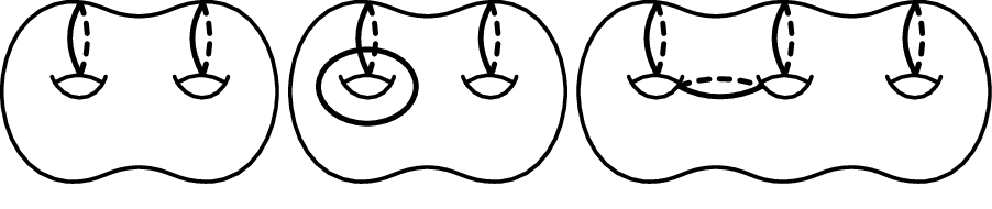
Definition 1.4.

The complex $\text{$\mathcal{MC}$}_{g}$ is the simplicial complex whose $(k-1)$ -simplices are sets $\{\gamma_{1},\ldots,\gamma_{k}\}$ of isotopy classes of simple closed nonseparating curves on $\Sigma_{g}$ satisfying one of the following three conditions (for some ordering of the $\gamma_{i}$ ).

•

The $\gamma_{i}$ are disjoint and $\gamma_{1}\cup\cdots\cup\gamma_{k}$ does not separate $\Sigma_{g}$ (see Figure 4.a).
•

The $\gamma_{i}$ satisfy

$\text{$i_{\text{geom}}$}(\gamma_{i},\gamma_{j})=\begin{cases}1&\text{if $(i,j)=(1,2)$}\\ 0&\text{otherwise}\end{cases}$

and $\gamma_{1}\cup\cdots\cup\gamma_{k}$ does not separate $\Sigma_{g}$ (see Figure 4.b).
•

The $\gamma_{i}$ are disjoint, $\gamma_{1}\cup\gamma_{2}\cup\gamma_{3}$ cuts off a copy of $\Sigma_{0,3}$ from $\Sigma_{g}$ , and $\{\gamma_{1},\ldots,\gamma_{k}\}\setminus\{\gamma_{1}\}$ is a standard simplex (see Figure 4.c).

Our main result about $\text{$\mathcal{MC}$}_{g}$ (Proposition 4.4 below) says that $\text{$\mathcal{MC}$}_{g}/\text{${\mathcal{I}}$}_{g}$ is $(g-1)$ -connected. In particular, it is $2$ -connected for $g=3$ .

History and comments.

Three additional results concerning presentations of the Torelli group should be mentioned. First, Krstić and McCool [19] have proven that the analogue of the Torelli group in $\Aut(F_{n})$ is not finitely presentable for $n=3$ . Second, using algebreo-geometric methods, Hain [10] has computed a finite presentation for the Malcev Lie algebra of $\text{${\mathcal{I}}$}_{g}$ for $g\geq 6$ . Finally, in addition to their infinite presentation of the Torelli group, Morita and Penner [26] used Johnson’s finite generating set for the Torelli group to give a finite presentation of the fundamental groupoid of a certain cell decomposition of the quotient of Teichmüller space by the Torelli group.

As far as relations in the Torelli group go, Johnson’s paper [17] contains a veritable zoo of relations, most of which are derived from clever combinations of lantern relations in the mapping class group. An excellent discussion of these relations, plus some generalizations of them, can be found in Brendle’s unpublished thesis [5]. The rest of our relations seem to be new, though it is unclear which of them can be derived from Johnson’s relations.

We finally wish to draw attention to a paper of Gervais [9] that constructs an infinite presentation for the whole mapping class group using the set of all Dehn twists as generators. Gervais’s presentation was later simplified by Luo [20].

Outline.

We begin in §2 with a review of the Birman exact sequence together with some basic group theory. Next, in §3 we derive the nonformal relations in our presentation. The proof of Theorem 1.2 is in §4. This proof depends on two propositions that are proven in §5 and §6.

Conventions and notation.

All homology groups will have $\mathbb{Z}$ coefficients. Throughout this paper, we will systematically confuse simple closed curves with their homotopy classes. Hence (based/unbased) curves are said to be simple closed curves if they are (based/unbased) homotopic to simple closed curves, etc. If $\gamma_{1}$ and $\gamma_{2}$ are two simple closed curves, then $\text{$i_{\text{geom}}$}(\gamma_{1},\gamma_{2})$ will denote the geometric intersection number of $\gamma_{1}$ and $\gamma_{2}$ ; i.e. the minimum over all curves $\gamma_{1}^{\prime}$ and $\gamma_{2}^{\prime}$ with $\gamma_{i}^{\prime}$ isotopic to $\gamma_{i}$ for $1\leq i\leq 2$ of the number of points of $\gamma_{1}^{\prime}\cap\gamma_{2}^{\prime}$ . If $\gamma_{1}$ and $\gamma_{2}$ are either oriented simple closed curves or elements of $\HH_{1}(\Sigma_{g})$ , then $\text{$i_{\text{alg}}$}(\gamma_{1},\gamma_{2})$ will denote the algebraic intersection number of $\gamma_{1}$ and $\gamma_{2}$ . Finally, we will say that $x,y\in\pi_{1}(\Sigma_{g,n})$ are completely distinct if $x\neq y$ and $x\neq y^{-1}$ .

For surfaces with boundary, the group $\Mod_{g,n}$ is defined to be the group of homotopy classes of orientation-preserving homeomorphisms of $\Sigma_{g,n}$ that fix the boundary pointwise (the homotopies also must fix the boundary). Like in the closed surface case, the group $\text{${\mathcal{I}}$}_{g,1}$ is defined to be the subgroup of $\Mod_{g,1}$ consisting of mapping classes that act trivially on $\HH_{1}(\Sigma_{g,1})$ . For surfaces with more than 1 boundary component, there is more than one useful definition for the Torelli group (see [29] for a discussion). We discuss one special definition in §3.2.1. As far group-theoretic conventions go, we define $[g_{1},g_{2}]=g_{1}^{-1}g_{2}^{-1}g_{1}g_{2}$ and $g_{1}^{g_{2}}=g_{2}^{-1}g_{1}g_{2}$ . Finally, we wish to draw the reader’s attention to the warning at the end of §2.1; it is the source of several somewhat counterintuitive formulas.

Acknowledgements.

I wish to thank my advisor Benson Farb for his enthusiasm and encouragement and for commenting extensively on previous incarnations of this paper. I also wish to thank Joan Birman, Matt Day, Martin Kassabov, Justin Malestein, and Ben Wieland for their comments on this project. I particularly wish to thank an anonymous referee for a very careful reading and many useful suggestions. Finally, I wish to thank the Department of Mathematics of the Georgia Institute of Technology for their hospitality during the time in which parts of this paper were conceived.

2 Preliminaries

2.1 The Birman exact sequence

In this section, we review the exact sequences of Birman and Johnson [2, 4, 17] that describe the effect on the mapping class group of gluing a disc to a boundary component; these will be the basis for our inductive arguments. We will need the following definition.

Definition 2.1.

Consider a surface $\Sigma_{g,n}$ . Let $\ast\in\Sigma_{g,n}$ be a point. We define $\Mod_{g,n}^{\ast}$ , the mapping class group relative to $\ast$ , to be the group of orientation-preserving homeomorphisms of $\Sigma_{g,n}$ that fix $\ast$ and the boundary pointwise modulo isotopies fixing $\ast$ and the boundary pointwise.

Let $b$ be a boundary component of $\Sigma_{g,n}$ . There is a natural embedding $\Sigma_{g,n}\hookrightarrow\Sigma_{g,n-1}$ induced by gluing a disc to $b$ . Let $\ast\in\Sigma_{g,n-1}$ be a point in the interior of the new disc. Clearly we can factor the induced map $\Mod_{g,n}\rightarrow\Mod_{g,n-1}$ into a composition

\Mod_{g,n}\longrightarrow\Mod_{g,n-1}^{\ast}\longrightarrow\Mod_{g,n-1}.

Now let $U\Sigma_{g,n-1}$ be the unit tangent bundle of $\Sigma_{g,n-1}$ and $\tilde{\ast}$ be any lift of $\ast$ to $U\Sigma_{g,n-1}$ . The combined work of Birman [2] and Johnson [17] shows that (except for the degenerate cases where $(g,n)$ equals $(0,1)$ , $(0,2)$ , or $(1,1)$ ) all of our groups fit into the following commutative diagram with exact rows and columns.

		$1$		$1$
		$\downarrow$		$\downarrow$
		$\mathbb{Z}$	$=$	$\mathbb{Z}$
		$\downarrow$		$\downarrow$
$1$	$\longrightarrow$	$\pi_{1}(U\Sigma_{g,n-1},\tilde{\ast})$	$\longrightarrow$	$\Mod_{g,n}$	$\longrightarrow$	$\Mod_{g,n-1}$	$\longrightarrow$	$1$
		$\downarrow$		$\downarrow$		$\parallel$
$1$	$\longrightarrow$	$\pi_{1}(\Sigma_{g,n-1},\ast)$	$\longrightarrow$	$\Mod_{g,n-1}^{\ast}$	$\longrightarrow$	$\Mod_{g,n-1}$	$\longrightarrow$	$1$
		$\downarrow$		$\downarrow$
		$1$		$1$

The $\mathbb{Z}$ in the first column is the loop in the fiber, while the $\mathbb{Z}$ in the second column corresponds to the Dehn twist about the filled-in boundary component. For $\gamma\in\pi_{1}(\Sigma_{g,n-1},\ast)$ , let $\overline{\text{Push}}(\gamma)$ be the element of $\Mod_{g,n-1}^{\ast}$ associated to $\gamma$ (hence $\overline{\text{Push}}(\gamma)$ “drags $\ast$ around the curve $\gamma$ ”). If $\gamma$ is nontrivial and can be represented by a simple closed curve, then there is a nice formula for $\overline{\text{Push}}(\gamma)$ (see Figures 5.a–c). Namely, let $\gamma_{1}$ and $\gamma_{2}$ be the boundary of a regular neighborhood of $\gamma$ . The orientation of $\gamma$ induces an orientation on $\gamma_{1}$ and $\gamma_{2}$ ; assume that $\gamma$ lies to the left of $\gamma_{1}$ and to the right of $\gamma_{2}$ . Then $\text{$\overline{\text{Push}}(\gamma)$}=T_{\gamma_{1}}T_{\gamma_{2}}^{-1}$ .

Continue to assume that $\gamma\neq 1$ can be represented by a simple closed curve. Recall that we have been considering $\Sigma_{g,n-1}$ to be $\Sigma_{g,n}$ with a disc glued to $b$ . In the other direction, we can consider $\Sigma_{g,n}$ to be $\Sigma_{g,n-1}$ with the point $\ast$ blown up to a boundary component (i.e. replaced with its circle of unit tangent vectors). Two such identifications of $\Sigma_{g,n}$ with a blow-up of $\Sigma_{g,n-1}$ may differ by a power of $T_{b}$ ; however, since $T_{b}$ fixes both $\gamma_{1}$ and $\gamma_{2}$ there are well-defined lifts $\tilde{\gamma}_{1}$ and $\tilde{\gamma}_{2}$ of the $\gamma_{i}$ to $\Sigma_{g,n}$ (see Figure 5.d). It is not hard to see that $\text{$\text{Push}(\gamma)$}:=T_{\tilde{\gamma}_{1}}T_{\tilde{\gamma}_{2}}^{-1}$ is a lift of $\overline{\text{Push}}(\gamma)$ .

Warning.

It is traditional to compose elements of $\pi_{1}$ from left to right (concatenation order) but to compose mapping classes from right to left (functional order). We will (reluctantly) adhere to these conventions, but because of them the map $\pi_{1}(U\Sigma_{g,n-1})\rightarrow\Mod_{g,n}$ and all other maps derived from it are anti-homomorphisms; i.e. they reverse the order of composition.

2.2 Two group-theoretic lemmas

In this section, we prove two easy group-theoretic lemmas that will form the basis for many of our arguments. The first is a tool for proving that sequences are exact.

Lemma 2.2.

Let $j:G_{2}\rightarrow G_{3}$ be a surjective homomorphism between two groups $G_{2}$ and $G_{3}$ , and let $G_{1}$ be a normal subgroup of $G_{2}$ with $G_{1}\subset\Ker(j)$ . Additionally, let $\langle S_{3}|R_{3}\rangle$ be a presentation for $G_{3}$ and $S_{2}$ be a generating set for $G_{2}$ satisfying $j(S_{2})=S_{3}$ . Assume that the following two conditions are satisfied.

1.

For all $s,s^{\prime}\in S_{2}\cup\{1\}$ with $j(s)=j(s^{\prime})$ , there exist $k_{1},k_{2}\in G_{1}$ so that $s=k_{1}s^{\prime}k_{2}$ .
2.

For any relation $r_{1}\cdots r_{k}\in R_{3}$ , we can find $\tilde{r}_{1},\ldots,\tilde{r}_{k}\in S_{2}^{\pm 1}$ with $\tilde{r}_{1}\cdots\tilde{r}_{k}=1$ so that $j(\tilde{r}_{i})=r_{i}$ for $1\leq i\leq k$ .

Then the sequence

1\longrightarrow G_{1}\longrightarrow G_{2}\stackrel{{\scriptstyle j}}{{\longrightarrow}}G_{3}\longrightarrow 1

is exact.

Proof.

Let $\overline{S}_{2}\subset G_{2}/G_{1}$ be the projection of $S_{2}$ . By condition 1 the induced map $\overline{j}:G_{2}/G_{1}\rightarrow G_{3}$ restricts to a bijection between $\overline{S}_{2}$ and $S_{3}$ . Condition 2 then implies that there is an inverse $\overline{j}^{-1}$ ; i.e. that $\overline{j}$ is an isomorphism, as desired. ∎

Remark.

In the first condition of Lemma 2.2, since $G_{1}$ is normal it is enough to assume that there exists some $k\in G_{1}$ so that $s=s^{\prime}k$ . We stated it the way we did to make the logic behind some of our applications clearer.

The following special case of Lemma 2.2 will be used repeatedly.

Corollary 2.3.

Let $j:G_{2}\rightarrow G_{3}$ be a surjective homomorphism between two groups. Assume that $G_{3}$ has a presentation $\langle S_{3}|R_{3}\rangle$ and that $G_{2}$ has a generating set $S_{2}$ so that $j$ restricts to a bijection between $S_{2}$ and $S_{3}$ . Furthermore, assume that every relation $r_{1}\cdots r_{k}\in R_{3}$ (here $r_{i}\in S_{3}^{\pm 1}$ ) satisfies $j^{-1}(r_{1})\cdots j^{-1}(r_{k})=1$ , where $j^{-1}(r_{i})$ is the unique element of $S_{2}^{\pm 1}$ that is mapped to $r_{i}$ . Then $j$ is an isomorphism.

Corollary 2.3 is interesting even if $G_{3}$ is a free group – it says that if $j:G\rightarrow F(S)$ is a homomorphism from a group $G$ to the free group $F$ on the free generating set $S$ and if for each $s\in S$ there is some $\tilde{s}\in j^{-1}(s)$ so that the set $\{\text{$\tilde{s}$ $|$ $s\in S$}\}$ generates $G$ , then $j$ is an isomorphism.

The second lemma is a tool for proving that a set of elements generates a group.

Lemma 2.4.

Let $G$ be a group generated by a set $S$ . Assume that a group $H$ generated by a set $T$ acts on $G$ (as a set, not necessarily as a group) and that $S^{\prime}\subset S$ satisfies the following two conditions.

1.

$H(S^{\prime})=S$
2.

For $t\in T^{\pm 1}$ and $s\in S^{\prime}$ , we have $t(s)\in\text{$\langle\text{$S^{\prime}$}\rangle$}\subset G$ .

Then $S^{\prime}$ generates $G$ .

Proof.

By condition 2, the group $H$ stabilizes $\text{$\langle\text{$S^{\prime}$}\rangle$}\subset G$ . Condition 1 then implies that $S\subset\text{$\langle\text{$S^{\prime}$}\rangle$}$ , so $\text{$\langle\text{$S^{\prime}$}\rangle$}=G$ , as desired. ∎

3 Non-formal relations in the Torelli group

In this section, we derive the non-formal relations in our presentation.

Remark.

As will become clear, all the non-formal relations in our presentation arise in some fashion from the Birman exact sequence.

3.1 The lantern and crossed lantern relations

3.1.1 Preliminaries

We first discuss relations that arise from “dragging subsurfaces around”. Fix a simple closed separating curve $b$ on $\Sigma_{g}$ . Cutting $\Sigma_{g}$ along $b$ , we obtain subsurfaces homeomorphic to $\Sigma_{h_{1},1}$ and $\Sigma_{h_{2},1}$ for some integers $h_{1}$ and $h_{2}$ satisfying $h_{1}+h_{2}=g$ . Assume that $h_{1}>0$ and $h_{2}>1$ . Observe that we have an injection $\text{${\mathcal{I}}$}_{h_{2},1}\hookrightarrow\text{${\mathcal{I}}$}_{g}$ . Additionally, the formulas in §2.1 imply that the kernel $\pi_{1}(U\Sigma_{h_{2}})$ of the Birman exact sequence for $\Sigma_{h_{2},1}$ lies in $\text{${\mathcal{I}}$}_{h_{2},1}$ , so we have an exact sequence

1\longrightarrow\pi_{1}(U\Sigma_{h_{2}})\longrightarrow\text{${\mathcal{I}}$}_{h_{2},1}\longrightarrow\text{${\mathcal{I}}$}_{h_{2}}\longrightarrow 1.

(1)

Combining these two observations, we obtain an injection $\pi_{1}(U\Sigma_{h_{2}})\hookrightarrow\text{${\mathcal{I}}$}_{g}$ . The element of $\Mod_{g}$ that corresponds to $\gamma\in\pi_{1}(U\Sigma_{h_{2}})$ can be informally described as “dragging $\Sigma_{h_{1},1}$ around $\gamma$ ”. We will construct relations in $\pi_{1}(U\Sigma_{h_{2}})$ using the push-maps discussed in §2.1 and then use the aforementioned injection to map these relations into $\text{${\mathcal{I}}$}_{g}$ .

3.1.2 The lantern relation

Consider simple closed curves $x,y,z\in(\pi_{1}(\Sigma_{h_{2}})\setminus\{1\})$ that can be arranged like the curves drawn in Figure 3.a. Observe that $xyz=1$ and that

\text{$\text{Push}(x)$}=T_{\tilde{x}_{1},\tilde{x}_{2}}\in\pi_{1}(U\Sigma_{h_{2}})

for the curves $\tilde{x}_{1}$ and $\tilde{x}_{2}$ depicted in Figure 3.c. Similar statements are true for $y$ and $z$ . We conclude that in $\pi_{1}(U\Sigma_{h_{2}})\subset\text{${\mathcal{I}}$}_{g}$ , we must have

T_{\tilde{z}_{1},\tilde{z}_{2}}T_{\tilde{y}_{1},\tilde{y}_{2}}T_{\tilde{x}_{1},\tilde{x}_{2}}=T_{b}^{k}

for some $k$ (observe that we have switched the order of composition here from concatenation order for curves to functional order for mapping classes). By examining the action on a properly embedded arc exactly one of whose endpoints lies on $b$ , one can check that $k=1$ . These are the classical lantern relations (see, e.g., [14]). Summing up, we have

T_{\tilde{z}_{1},\tilde{z}_{2}}T_{\tilde{y}_{1},\tilde{y}_{2}}T_{\tilde{x}_{1},\tilde{x}_{2}}=T_{b}\\

(L)

for all curves $\tilde{x}_{1}$ , $\tilde{x}_{2}$ , $\tilde{y}_{1}$ , $\tilde{y}_{2}$ , $\tilde{z}_{1}$ , and $\tilde{z}_{2}$ embedded in $\Sigma_{g}$ like the curves in Figure 3.c.

Remark.

This interpretation of the lantern relation was discovered independently by Margalit and McCammond [23].

3.1.3 The crossed lantern relation

Now consider simple closed curves $x,y,z\in(\pi_{1}(\Sigma_{h_{2}})\setminus\{1\})$ that can be arranged like the curves drawn in Figure 3.b. Observe that $xy=z$ and that

\text{$\text{Push}(x)$}=T_{\tilde{x}_{1}}T_{\tilde{x}_{2}}^{-1}\in\pi_{1}(U\Sigma_{h_{2}})\subset\text{${\mathcal{I}}$}_{g}

for the curves $\tilde{x}_{1}$ and $\tilde{x}_{2}$ depicted in Figure 3.d. Similar statements are true for $y$ and $z$ . We conclude that in $\pi_{1}(U\Sigma_{h_{2}})\subset\text{${\mathcal{I}}$}_{g}$ , we must have

(T_{\tilde{y}_{1}}T_{\tilde{y}_{2}}^{-1})(T_{\tilde{x}_{1}}T_{\tilde{x}_{2}}^{-1})=(T_{\tilde{z}_{1}}T_{\tilde{z}_{2}}^{-1})T_{b}^{k}

for some $k$ . By examining the action on a properly embedded arc exactly one of whose endpoints lies on $b$ , one can check that $k=0$ . We will call these the crossed lantern relations. Summing up, our relation is

T_{\tilde{y}_{1},\tilde{y}_{2}}T_{\tilde{x}_{1},\tilde{x}_{2}}=T_{\tilde{z}_{1},\tilde{z}_{2}}\\

(CL)

for all curves $\tilde{x}_{1}$ , $\tilde{x}_{2}$ , $\tilde{y}_{1}$ , $\tilde{y}_{2}$ , $\tilde{z}_{1}$ , and $\tilde{z}_{2}$ that can be embedded in $\Sigma_{g}$ like the curves depicted in Figure 3.d.

Alternate Derivation.

Observe that for $i=1,2$ we have $\tilde{z}_{i}=T_{\tilde{x}_{2}}(\tilde{y}_{i})$ . Expanding out the $T_{\tilde{z}_{1},\tilde{z}_{2}}$ in (CL) as $T_{\tilde{x}_{2}}T_{\tilde{y}_{1},\tilde{y}_{2}}T_{\tilde{x}_{2}}^{-1}$ and rearranging terms, we see that (CL) is equivalent to $T_{\tilde{y}_{1},\tilde{y}_{2}}T_{\tilde{x}_{1}}T_{\tilde{y}_{1},\tilde{y}_{2}}^{-1}=T_{\tilde{x}_{2}}$ . This follows from the easily verified identity $T_{\tilde{y}_{1},\tilde{y}_{2}}(\tilde{x}_{1})=\tilde{x}_{2}$ .

3.2 The Witt–Hall and commutator shuffle relations

3.2.1 Preliminaries

We now examine the relations that arise from “dragging the end of a handle”. For use later in §5.1, we will discuss a slightly more general situation. For $g\geq 0$ and $n\geq 2$ , let $i:\Sigma_{g,n}\hookrightarrow\Sigma_{g+n-1}$ be the embedding of $\Sigma_{g,n}$ into the surface obtained by gluing the boundary components of a copy of $\Sigma_{0,n}$ to the boundary components of $\Sigma_{g,n}$ . Define $\text{${\mathcal{I}}$}_{g,n}=i_{\ast}^{-1}(\text{${\mathcal{I}}$}_{g+n-1})$ . It is not hard to see that this is well-defined. Observe that $i_{\ast}(\text{${\mathcal{I}}$}_{g,2})$ is the subgroup of $\text{${\mathcal{I}}$}_{g+1}$ stabilizing the handle corresponding to the glued-in annulus. The groups $\text{${\mathcal{I}}$}_{g,n}$ were introduced by Johnson [18] and investigated further by van den Berg [34] and the author [29] (in the notation of [29], if the boundary components of $\Sigma_{g,n}$ are $\{b_{1},\ldots,b_{n}\}$ , then $\text{${\mathcal{I}}$}_{g,n}=\text{${\mathcal{I}}$}(\Sigma_{g,n},\{\{b_{1},\ldots,b_{n}\}\})$ ).

We will say that a mapping class $f\in\Mod_{g,n}$ is a separating twist, etc., if $i_{\ast}(f)$ is a separating twist, etc. It follows from [29, Theorem 1.3] that if $g\geq 1$ , then separating twists and bounding pair maps generate $\text{${\mathcal{I}}$}_{g,n}$ .

Remark.

Not all simple closed curves that separate $\Sigma_{g,n}$ are nullhomologous. By our definition, separating twists in $\Mod_{g,n}$ are exactly Dehn twists about nullhomologous simple closed curves.

Let $b$ be a boundary component of $\Sigma_{g,n}$ . The kernel $\pi_{1}(U\Sigma_{g,n-1})$ of the map $\Mod_{g,n}\rightarrow\Mod_{g,n-1}$ induced by gluing a disc to $b$ does not lie in $\text{${\mathcal{I}}$}_{g,n}$ (for instance, $T_{b}\notin\text{${\mathcal{I}}$}_{g,n}$ ). Instead, [29, Theorem 4.1] says that we have an exact sequence

1\longrightarrow[\pi_{1}(\Sigma_{g,n-1}),\pi_{1}(\Sigma_{g,n-1})]\longrightarrow\text{${\mathcal{I}}$}_{g,n}\longrightarrow\text{${\mathcal{I}}$}_{g,n-1}\longrightarrow 1.

(2)

The group $[\pi_{1}(\Sigma_{g,n-1}),\pi_{1}(\Sigma_{g,n-1})]$ is embedded in $\pi_{1}(U\Sigma_{g,n-1})\cong\pi_{1}(\Sigma_{g,n-1})\otimes\text{$\mathbb{Z}$}$ as the graph of a homomorphism $\phi:[\pi_{1}(\Sigma_{g,n-1}),\pi_{1}(\Sigma_{g,n-1})]\rightarrow\text{$\mathbb{Z}$}$ , that is, as the set of all pairs $(x,\phi(x))$ for $x\in[\pi_{1}(\Sigma_{g,n-1}),\pi_{1}(\Sigma_{g,n-1})]$ . The identification $\pi_{1}(U\Sigma_{g,n-1})\cong\pi_{1}(\Sigma_{g,n-1})\otimes\text{$\mathbb{Z}$}$ (or, equivalently, the splitting $\pi_{1}(\Sigma_{g,n-1})\rightarrow\pi_{1}(U\Sigma_{g,n-1})$ of the natural surjection $\pi_{1}(U\Sigma_{g,n-1})\rightarrow\pi_{1}(\Sigma_{g,n-1})$ ) is not natural, but once a splitting $\rho:\pi_{1}(\Sigma_{g,n-1})\rightarrow\pi_{1}(U\Sigma_{g,n-1})$ is chosen $\phi$ is uniquely defined by the requirement that the image of the homomorphism $[\pi_{1}(\Sigma_{g,n-1}),\pi_{1}(\Sigma_{g,n-1})]\rightarrow\pi_{1}(U\Sigma_{g,n-1})$ defined by $x\mapsto\rho(x)T_{b}^{\phi(x)}$ must be contained in the pullback of $\text{${\mathcal{I}}$}_{g,n}$ under the inclusion $\pi_{1}(U\Sigma_{g,n-1})\hookrightarrow\Mod_{g,n}$ .

For curves $\gamma^{1},\gamma^{2}\in(\pi_{1}(\Sigma_{g,n-1})\setminus\{1\})$ , define $\llbracket\gamma^{1},\gamma^{2}\rrbracket$ to be the element of $\text{${\mathcal{I}}$}_{g,n}$ associated to $[\gamma^{1},\gamma^{2}]$ . To simplify our notation, if $\eta\in\pi_{1}(\Sigma_{g,n-1})$ is another simple closed curve, then we define

\text{$\llbracket\gamma^{1},\gamma^{2}\rrbracket$}^{\eta}:=\text{$\llbracket(\eta^{-1})(\gamma^{1})(\eta),(\eta^{-1})(\gamma^{2})(\eta)\rrbracket$}=\text{$\llbracket\text{$\overline{\text{Push}}(\eta)$}(\gamma^{1}),\text{$\overline{\text{Push}}(\eta)$}(\gamma^{2})\rrbracket$}.

Finally, if $\gamma\in(\pi_{1}(\Sigma_{g,n-1})\setminus\{1\})$ is already an element of the commutator subgroup, then let $\llbracket\gamma\rrbracket$ be the element of $\text{${\mathcal{I}}$}_{g,n}$ associated to $\gamma$ .

We will need some explicit formulas for $\llbracket\cdot,\cdot\rrbracket$ . Consider two completely distinct simple closed curves $\gamma^{1},\gamma^{2}\in(\pi_{1}(\Sigma_{g,n-1})\setminus\{1\})$ that only intersect at the base point. From the above description, we see that the following procedure will yield $\llbracket\gamma^{1},\gamma^{2}\rrbracket$ .

1.

Choose some $\psi\in\Mod_{g,n}$ which is associated to an element of $\pi_{1}(U\Sigma_{g,n-1})$ that projects to $[\gamma^{1},\gamma^{2}]\in\pi_{1}(\Sigma_{g,n-1})$ .
2.

Determine $k\in\text{$\mathbb{Z}$}$ so that $\psi T_{b}^{k}\in\text{${\mathcal{I}}$}_{g,n}$ . We will then have $\text{$\llbracket\gamma^{1},\gamma^{2}\rrbracket$}=\psi T_{b}^{k}$ .

There are two cases. In the first (see Figure 6.a), a regular neighborhood of $\gamma^{1}\cup\gamma^{2}$ is homeomorphic to $\Sigma_{1,1}$ . Observe that $[\gamma^{1},\gamma^{2}]$ is homotopic to a simple closed separating curve. Our element $\psi$ in this case will be $\text{Push}([\gamma^{1},\gamma^{2}])$ . Observe that

\text{$\text{Push}([\gamma^{1},\gamma^{2}])$}=T_{\widetilde{[\gamma^{1},\gamma^{2}]}_{1}}T_{\widetilde{[\gamma^{1},\gamma^{2}]}_{2}}^{-1}

for simple closed curves $\widetilde{[\gamma^{1},\gamma^{2}]}_{1}$ and $\widetilde{[\gamma^{1},\gamma^{2}]}_{2}$ like the curves pictured in Figure 6.b.

Note that exactly one element of the pair $\{\widetilde{[\gamma^{1},\gamma^{2}]}_{1},\widetilde{[\gamma^{1},\gamma^{2}]}_{2}\}$ is a separating curve (both curves separate $\Sigma_{g,n}$ , but only one of them maps to a separating curve on $\Sigma_{g+n-1}$ ). In Figure 6.b, the curve $\widetilde{[\gamma^{1},\gamma^{2}]}_{2}$ is separating, but in other situations $\widetilde{[\gamma^{1},\gamma^{2}]}_{1}$ will be the separating curve (for instance, this will happen if we flip the labels on the curves $\gamma^{1}$ and $\gamma^{2}$ in Figure 6.a). Now, the nonseparating curve and $b$ form a bounding pair on $\Sigma_{g,n}$ . We conclude that either

\text{$\llbracket\gamma^{1},\gamma^{2}\rrbracket$}=T_{\widetilde{[\gamma^{1},\gamma^{2}]}_{1},b}T_{\widetilde{[\gamma^{1},\gamma^{2}]}_{2}}^{-1}

\text{$\llbracket\gamma^{1},\gamma^{2}\rrbracket$}=T_{\widetilde{[\gamma^{1},\gamma^{2}]}_{1}}T_{b,\widetilde{[\gamma^{1},\gamma^{2}]}_{2}},

depending on which curve is separating. In a similar way, if $\gamma$ is a separating curve then $\llbracket\gamma\rrbracket$ equals the product of a separating twist and a bounding pair map.

In the second case, a regular neighborhood of $\gamma^{1}\cup\gamma^{2}$ is homeomorphic to $\Sigma_{0,3}$ (see Figure 6.c). In this case, our element $\psi$ will be

\text{$\text{Push}(\gamma^{2})$}\text{$\text{Push}(\gamma^{1})$}\text{$\text{Push}(\gamma^{2})$}^{-1}\text{$\text{Push}(\gamma^{1})$}^{-1}.

Lifting everything to $\Sigma_{g,n}$ , we see that

\text{$\text{Push}(\gamma^{i})$}=T_{\tilde{\gamma}^{i}_{1}}^{e_{i}}T_{\tilde{\gamma}^{i}_{2}}^{-e_{i}}

for the curves depicted in Figure 6.d and some $e_{i}=\pm 1$ (the $e_{i}$ depend on the orientations of $\gamma^{1}$ and $\gamma^{2}$ ). Observe that

\text{$\text{Push}(\gamma^{2})$}\text{$\text{Push}(\gamma^{1})$}\text{$\text{Push}(\gamma^{2})$}^{-1}\text{$\text{Push}(\gamma^{1})$}^{-1}=T_{\tilde{\gamma}^{2}_{1}}^{e_{2}}T_{\tilde{\gamma}^{1}_{1}}^{e_{1}}T_{\tilde{\gamma}^{2}_{1}}^{-e_{2}}T_{\tilde{\gamma}^{1}_{1}}^{-e_{1}}=[T_{\tilde{\gamma}^{2}_{1}}^{-e_{i}},T_{\tilde{\gamma}^{1}_{1}}^{-e_{i}}]\in\text{${\mathcal{I}}$}_{g,n}.

We conclude that $\text{$\llbracket\gamma^{1},\gamma^{2}\rrbracket$}=[T_{\tilde{\gamma}^{2}_{1}}^{-e_{2}},T_{\tilde{\gamma}^{1}_{1}}^{-e_{2}}]$ . Now, this is the commutator of the simply intersecting pair $\{\tilde{\gamma}^{2}_{1},\tilde{\gamma}^{1}_{1}\}$ if $e_{2}=e_{1}=-1$ ; we will call a pair of curves $\gamma^{1}$ and $\gamma^{2}$ with this property positively aligned. If $\gamma^{1}$ and $\gamma^{2}$ are not positively aligned, however, then by repeatedly applying the commutator identity $[g_{1}^{-1},g_{2}]=[g_{2},g_{1}]^{g_{1}^{-1}}$ and the fact that $T_{x}T_{y}T_{x}^{-1}=T_{T_{x}(y)}$ for simple closed curves $x$ and $y$ , we can find a simply intersecting pair $C_{\rho^{1},\rho^{2}}$ with $\text{$\llbracket\gamma^{1},\gamma^{2}\rrbracket$}=C_{\rho^{1},\rho^{2}}$ . We conclude that $\llbracket\gamma^{1},\gamma^{2}\rrbracket$ is a commutator of some simply intersecting pair no matter how $\gamma^{1}$ and $\gamma^{2}$ are aligned.

Example 3.1.

We can now give an example of the non-uniqueness of the expression of a mapping class as a commutator of a simply intersecting pair. Orienting $\gamma^{1}$ and $\gamma^{2}$ as shown in Figure 6.a, we have $\text{$\llbracket(\gamma^{1})^{-1},(\gamma^{2})^{-1}\rrbracket$}=C_{\tilde{\gamma}^{2}_{1},\tilde{\gamma}^{1}_{1}}$ (verifying this is a good exercise in understanding the above construction). Let $\delta$ be the curve in Figure 6.e. Observe that $\text{$\llbracket(\gamma^{2})^{-1}(\gamma^{1})^{-1},(\gamma^{2})^{-1}\rrbracket$}=[T_{\tilde{\gamma}^{2}_{1}},T_{\delta}^{-1}]$ . Since we have the commutator identity $[(\gamma^{2})^{-1}(\gamma^{1})^{-1},(\gamma^{2})^{-1}]=[(\gamma^{1})^{-1},(\gamma^{2})^{-1}]$ , we conclude that $C_{\tilde{\gamma}^{2}_{1},\tilde{\gamma}^{1}_{1}}=[T_{\tilde{\gamma}^{2}_{1}},T_{\delta}^{-1}]$ . The right hand side of this is not a commutator of a simply intersecting pair, but the above procedure shows that it equals $C_{\delta,T_{\delta}^{-1}(\tilde{\gamma}^{2}_{1})}$ .

We conclude with the following lemma.

Lemma 3.2.

Let $s\in\text{${\mathcal{I}}$}_{g,n}$ be a commutator of a simply intersecting pair whose image under the map $\text{${\mathcal{I}}$}_{g,n}\rightarrow\text{${\mathcal{I}}$}_{g,n-1}$ is $1$ . Then there are completely distinct simple closed curves $\gamma^{1},\gamma^{2}\in\pi_{1}(\Sigma_{g,n-1})$ that only intersect at the basepoint so that $s=\text{$\llbracket\gamma^{1},\gamma^{2}\rrbracket$}$ .

Proof.

Let $s=C_{x,y}$ . Then a regular neighborhood $N$ of $x\cup y$ satisfies $N\cong\Sigma_{0,4}$ . Moreover, our assumptions imply that some boundary component of $N$ must be isotopic to $b$ . The lemma then follows from Figures 6.c–d and the above discussion. ∎

3.2.2 Witt–Hall relations

In this section and in §3.2.3, we will derive relations in the group $\text{${\mathcal{I}}$}_{g,2}$ . These relations give us relations in the Torelli groups of closed surfaces in the following way. For $g^{\prime}\geq g$ , let $\Sigma_{g,2}\hookrightarrow\Sigma_{g^{\prime}}$ be any embedding (not just the embedding $\Sigma_{g,2}\hookrightarrow\Sigma_{g+1}$ discussed in §3.2.1). There is then an induced map $\text{${\mathcal{I}}$}_{g,2}\rightarrow\text{${\mathcal{I}}$}_{g^{\prime}}$ (“extend by the identity”; see [29, Theorem Summary 1.1]). This induced map takes separating twists, bounding pair maps, and simply intersecting pair maps to generators of the same type (possibly degenerate ones, such as bounding pair maps $T_{x,y}$ with $x$ isotopic to $y$ ). If

s_{1}^{e_{1}}\cdots s_{k}^{e_{k}}=1\quad(e_{i}=\pm 1)

is a relation between separating twists, bounding pair maps, and simply intersecting pair maps in $\text{${\mathcal{I}}$}_{g,2}$ and $s_{i}^{\prime}$ is the image of $s_{i}$ in $\text{${\mathcal{I}}$}_{g^{\prime}}$ via the above map, then we obtain a relation between our generators in $\text{${\mathcal{I}}$}_{g^{\prime}}$ by deleting all the degenerate generators in the relation $(s_{1}^{\prime})^{e_{1}}\cdots(s_{k}^{\prime})^{e_{k}}=1$ .

The two families of relations that we derive from exact sequence (2) come from commutator identities. First, consider the Witt–Hall commutator identity

[g_{1}g_{2},g_{3}]=[g_{1},g_{3}]^{g_{2}}[g_{2},g_{3}].

Remark.

The Witt–Hall commutator identity first appeared in [11]. Later, it appeared in a list of basic commutator identities dubbed the “Witt–Hall identities” in [21].

Fix $x,y,z\in(\pi_{1}(\Sigma_{g,1})\setminus\{1\})$ so that for each of the sets $\{x,y,z\}$ and $\{xy,z\}$ , the elements of the set can be represented by completely distinct simple closed curves that only intersect at the basepoint. There are several different topological types of configurations of curves with these properties; an example is in Figure 7.a. The Witt–Hall commutator identity then yields the following relation, which we will call the Witt–Hall relation.

\text{$\llbracket xy,z\rrbracket$}=\text{$\llbracket y,z\rrbracket$}\text{$\llbracket x,z\rrbracket$}^{y}.\\

(WH)

We now give an example.

Example 3.3.

The curves $x$ , $y$ , and $z$ depicted in Figure 7.a satisfy the conditions for the Witt–Hall relations. In the surface group, the relation is $[xy,z]=[x,z]^{y}[y,z]$ . In Figure 7.b, we depict the curves involved in this surface group relation. Let $z_{1}$ , $(xy)_{2}$ , $c_{1}$ , $c_{2}$ , $a_{1}$ , and $a_{2}$ be the curves depicted in Figure 7.c. We then have $\text{$\text{Push}([x,z]^{y})$}=T_{a_{1},a_{2}}$ and $\text{$\text{Push}([y,z])$}=T_{c_{1},c_{2}}$ . The corresponding relation in Torelli is $[T_{z_{1}}^{-1},T_{(xy)_{2})}]=T_{c_{1},b}T_{c_{2}}^{-1}T_{a_{1}}T_{b,a_{2}}$ (the counterintuitive form of the initial commutator comes from the fact that the map from the kernel of the Birman exact sequence to Torelli is an anti-homomorphism). However, $[T_{z_{1}}^{-1},T_{(xy)_{2})}]$ is not a commutator of a simply intersecting pair (i.e. $z$ and $xy$ are not positively aligned). Using the relation $[g_{1}^{-1},g_{2}]=[g_{1}g_{2}g_{1}^{-1},g_{1}]$ , we transform this into the Witt–Hall relation $C_{T_{z_{1}}((xy)_{2}),z_{1}}=T_{c_{1},b}T_{c_{2}}^{-1}T_{a_{1}}T_{b,a_{2}}$ .

3.2.3 Commutator shuffle relations

We now use another, somewhat less standard commutator identity to find relations in the Torelli group. Our commutator identity, which is easily verified, is the following.

[g_{1},g_{2}]^{g_{3}}=[g_{3},g_{1}][g_{3},g_{2}]^{g_{1}}[g_{1},g_{2}][g_{1},g_{3}]^{g_{2}}[g_{2},g_{3}].

Though it may seem a bit odd, it will become apparent in §5.2.3 that this is exactly the relation we need to complete our picture. We will apply it to completely distinct simple closed curves $x,y,z\in(\pi_{1}(\Sigma_{g,1})\setminus\{1\})$ that only intersect at the basepoint. Again, there are finitely many topological types of such configurations. Our relation is then

\text{$\llbracket x,y\rrbracket$}^{z}=\text{$\llbracket y,z\rrbracket$}\text{$\llbracket x,z\rrbracket$}^{y}\text{$\llbracket x,y\rrbracket$}\text{$\llbracket z,y\rrbracket$}^{x}\text{$\llbracket z,x\rrbracket$}.\\

(CS)

We will call these relations the commutator shuffles. Pictures of them are left as an exercise for the reader.

4 The Main Theorem

4.1 A stronger version of the Main Theorem

To facilitate our induction, we will have to consider not only the case of a closed surface but also the case of a surface with boundary. In this section, we state a version of our Main Theorem that applies to these cases. We begin with a definition.

Definition 4.1.

For $g\geq 2$ and $n\geq 0$ , define $\Gamma_{g,n}$ to be the group whose generating set is the set of all separating twists, all bounding pair maps, and all commutators of simply intersecting pairs on $\Sigma_{g,n}$ and whose relations are the following. For $n=0$ , they are relations (F.1)-(F.8) from §1, relations (L) and (CL) from §3.1, and relations (WH) and (CS) from §3.2 (for the relations (WH) and (CS), we use all ways of “embedding them in the closed surface” as described in the beginning of §3.2.2). For $n=1$ , they are the set of all words $r$ in the generators of $\Gamma_{g,n}$ so that $i_{\ast}(r)$ is one of the above relations, where $i:\Sigma_{g,1}\hookrightarrow\Sigma_{g+1}$ is the embedding obtained by gluing a copy of $\Sigma_{1,1}$ to $\Sigma_{g,1}$ and $i_{\ast}$ is the obvious map defined on the generators. For $n>1$ , they are the set of all words $r$ in the generators of $\Gamma_{g,n}$ so that $i_{\ast}(r)$ is one of the above relations, where $i:\Sigma_{g,n}\hookrightarrow\Sigma_{g+n-1,1}$ obtained by gluing $n$ boundary components of a copy of $\Sigma_{0,n+1}$ to the boundary components of $\Sigma_{g,n}$ and $i_{\ast}$ is the obvious map defined on the generators.

Remark.

The generators for $\Gamma_{g,n}$ are mapping classes, not merely abstract symbols. For bounding pair maps and separating twists, this is unimportant, as their defining curves are determined by their mapping classes. For commutators of simply intersecting pairs, however, different pairs of curves determine the same mapping class (see Example 3.1), and we identify these in $\Gamma_{g,n}$ .

Since all of the relations of $\Gamma_{g,n}$ also hold in $\text{${\mathcal{I}}$}_{g,n}$ , there is a natural homomorphism $\Gamma_{g,n}\rightarrow\text{${\mathcal{I}}$}_{g,n}$ . A stronger version of Theorem 1.2 is then the following.

Theorem 4.2 (Main Theorem, Stronger Version).

For $n\leq 2$ and $g\geq 2$ , the natural map $\Gamma_{g,n}\rightarrow\text{${\mathcal{I}}$}_{g,n}$ is an isomorphism.

Remark.

In fact, this is also true for $n>2$ , but Theorem 4.2 is all we need. We will use the groups $\Gamma_{g,n}$ for $n>2$ later for technical purposes.

4.2 Obtaining presentations from group actions

In this section, we discuss a theorem of the author [30] that we will use to prove Theorem 4.2. In order to state it, we begin by noting that an argument of Armstrong [1] says that if $X$ is a simply connected simplicial complex and a group $G$ acts without rotations on $X$ (that is, for all simplices $s$ of $G$ the stabilizer $G_{s}$ stabilizes $s$ pointwise; this can be arranged by subdividing $X$ ), then if $X/G$ is also simply connected we can conclude that $G$ is generated by elements that stabilize vertices. In other words, we have a surjective map

\pi:\mathop{\text{\Huge{$\ast$}}}_{v\in X^{(0)}}G_{v}\longrightarrow G.

As notation, for $v\in X^{(0)}$ denote the inclusion map

G_{v}\hookrightarrow\mathop{\text{\Huge{$\ast$}}}_{v\in X^{(0)}}G_{v}

by $i_{v}$ .

There are then some obvious elements $\Ker(\pi)$ , which we write as relations $f=g$ rather than as elements $fg^{-1}$ . First, we have $i_{v}(g)i_{w}(h)i_{v}(g^{-1})=i_{g\cdot w}(ghg^{-1})$ for $g\in G_{v}$ and $h\in G_{w}$ . We call these relations the conjugation relations. Second, we have $i_{v}(g)=i_{v^{\prime}}(g)$ if $g\in G_{v}\cap G_{v^{\prime}}$ and $\{v,v^{\prime}\}\in X^{(1)}$ (here $\{v,v^{\prime}\}\in X^{(1)}$ means that $\{v,v^{\prime}\}$ forms an edge in the 1-skeleton of $X$ ). We call these the edge relations. The following theorem of the author says that under favorable circumstances these two families of relations yield the entire kernel of the aforementioned map.

Theorem 4.3 ([30]).

Let a group $G$ act without rotations on a simply connected simplicial complex $X$ . Assume that $X/G$ is $2$ -connected. Then

G=(\mathop{\text{\Huge{$\ast$}}}_{v\in X^{(0)}}G_{v})/R,

where $R$ is the normal subgroup generated by the conjugation relations and the edge relations.

4.3 The proof of the Main Theorem

In this section, we will give the outline of the proof of Theorem 4.2. Our main tool will be Theorem 4.3 together with two other results whose proofs are postponed until later sections.

The first major ingredient in our proof will be the following proposition, which is proven in §6. Recall that the complex $\text{$\mathcal{MC}$}_{g}$ was defined at the end of §1.

Proposition 4.4.

The simplicial complex $\text{$\mathcal{MC}$}_{g}$ satisfies the following two properties.

1.

The complex $\text{$\mathcal{MC}$}_{g}$ is $(g-2)$ -connected.
2.

The complex $\text{$\mathcal{MC}$}_{g}/\text{${\mathcal{I}}$}_{g}$ is $(g-1)$ -connected.

Remark.

In fact, using similar methods one can prove that $\text{$\mathcal{C}$}_{g}/\text{${\mathcal{I}}$}_{g}$ is $(g-1)$ -connected, but Proposition 4.4 suffices for our purposes, and the details of its proof are less technical. In the end, one would get the same presentation no matter which of the two complexes one used.

Theorem 4.3 and Proposition 4.4 will allow us to give an inductive decomposition of $\text{${\mathcal{I}}$}_{g,n}$ . To show that the groups $\Gamma_{g,n}$ fit into this inductive picture, we will show that the groups $\Gamma_{g,n}$ fit into exact sequences like exact sequence (1) from §3.1.1 and exact sequence (2) from §3.2.1. More precisely, observe that there exist natural “disc-filling” homomorphisms $\Gamma_{g,1}\rightarrow\Gamma_{g}$ and $\Gamma_{g,2}\rightarrow\Gamma_{g,1}$ (defined on the generators). In §5, we will prove the following.

Proposition 4.5.

The aforementioned homomorphisms fit into the following exact sequences.

	$\displaystyle 1\longrightarrow\pi_{1}(U\Sigma_{g})\longrightarrow\Gamma_{g,1}\longrightarrow\Gamma_{g}\longrightarrow 1,$		(3)
	$\displaystyle 1\longrightarrow[\pi_{1}(\Sigma_{g,1}),\pi_{1}(\Sigma_{g,1})]\longrightarrow\Gamma_{g,2}\longrightarrow\Gamma_{g,1}\longrightarrow 1.$		(4)

Next, we will need the following lemma, which forms part of Lemma 5.9 below.

Lemma 4.6.

For $g\geq 2$ and $0\leq n\leq 2$ , using the relations in $\Gamma_{g,n}$ we can write any commutator of a simply intersecting pair as a product of bounding pairs maps and separating twists.

Finally, we will need some results of Mess and Johnson about separating twists. Recall that by convention, all homology groups have $\mathbb{Z}$ -coefficients. Observe that if $\gamma$ is a separating curve on $\Sigma_{g}$ that cuts $\Sigma_{g}$ into two subsurfaces $S_{1}$ and $S_{2}$ , then we have an splitting

\HH_{1}(\Sigma_{g})\cong\HH_{1}(S_{1})\oplus\HH_{1}(S_{2}),

where the $\HH_{1}(S_{i})$ are symplectic $\mathbb{Z}$ -modules which are orthogonal with respect to the intersection form. We will call such a splitting a symplectic splitting. Observe that the symplectic splitting associated to $\gamma$ is a conjugacy invariant of $T_{\gamma}\in\text{${\mathcal{I}}$}_{g}$ . We then have the following two theorems.

Theorem 4.7 (Mess, [25]).

$\text{${\mathcal{I}}$}_{2}$ is an infinitely generated free group. Moreover, there exists a free generating set of separating twists $S$ containing exactly one separating twist associated to each symplectic splitting of $\HH_{1}(\Sigma_{2})$ .

Theorem 4.8 (Johnson, [15]).

For $g\geq 2$ , two separating twists $T_{\gamma_{1}}$ and $T_{\gamma_{2}}$ in $\text{${\mathcal{I}}$}_{g}$ are conjugate if and only if they induce the same symplectic splitting of $\HH_{1}(\Sigma_{g})$ .

We now assemble these ingredients to prove Theorem 4.2.

Proof of Theorem 4.2.

The proof will be by induction on $g$ and $n$ . We begin with the base case $(g,n)=(2,0)$ .

Claim 1.

The natural map $\Gamma_{2}\rightarrow\text{${\mathcal{I}}$}_{2}$ is an isomorphism.

Proof of Claim 1.

Observe first that $\Sigma_{2}$ does not contain any bounding pairs. Also, using Lemma 4.6 we see that $\Gamma_{2}$ is generated by separating twists. Let $S$ be the generating set for $\text{${\mathcal{I}}$}_{2}$ given by Theorem 4.7. Using the conjugation relation (F.6) together with Theorem 4.8, we conclude that $\Gamma_{g,2}$ is generated by $\{\text{$T_{\gamma}$ $|$ $\gamma\in S$}\}$ . Corollary 2.3 therefore implies that the natural map $\Gamma_{2}\rightarrow\text{${\mathcal{I}}$}_{2}$ is an isomorphism, as desired. ∎

Now assume by induction that for some $g\geq 2$ the natural map $\Gamma_{g}\rightarrow\text{${\mathcal{I}}$}_{g}$ is an isomorphism.

Claim 2.

The natural maps $\Gamma_{g,1}\rightarrow\text{${\mathcal{I}}$}_{g,1}$ and $\Gamma_{g,2}\rightarrow\text{${\mathcal{I}}$}_{g,2}$ are isomorphisms.

Proof of Claim 2.

Using Proposition 4.5, we have the following commutative diagram of exact sequences.

$1$	$\rightarrow$	$\pi_{1}(U\Sigma_{g})$	$\rightarrow$	$\Gamma_{g,1}$	$\rightarrow$	$\Gamma_{g}$	$\rightarrow$	$1$
		$\parallel$		$\downarrow$		$\downarrow$
$1$	$\rightarrow$	$\pi_{1}(U\Sigma_{g})$	$\rightarrow$	$\text{${\mathcal{I}}$}_{g,1}$	$\rightarrow$	$\text{${\mathcal{I}}$}_{g}$	$\rightarrow$	$1$

The right hand map is an isomorphism by induction, so the five lemma implies that the center map is an isomorphism; i.e. that $\Gamma_{g,1}\cong\text{${\mathcal{I}}$}_{g,1}$ . The proof that $\Gamma_{g,2}\cong\text{${\mathcal{I}}$}_{g,2}$ is similar. ∎

We now prove the following.

Claim 3.

The natural map $\Gamma_{g+1}\rightarrow\text{${\mathcal{I}}$}_{g+1}$ is an isomorphism.

Proof of Claim 3.

Since no two curves in a simplex of $\text{$\mathcal{MC}$}_{g+1}$ are homologous, the group $\text{${\mathcal{I}}$}_{g+1}$ acts on $\text{$\mathcal{MC}$}_{g+1}$ without rotations. Since $g+1\geq 3$ , Proposition 4.4 and Theorem 4.3 thus imply that

\text{${\mathcal{I}}$}_{g+1}\cong(\mathop{\text{\Huge{$\ast$}}}_{\text{$\gamma\in(\text{$\mathcal{MC}$}_{g+1})^{(0)}$}}(\text{${\mathcal{I}}$}_{g+1})_{\gamma})/R,

where $(\text{${\mathcal{I}}$}_{g+1})_{\gamma}$ denotes the stabilizer in $\text{${\mathcal{I}}$}_{g+1}$ of $\gamma$ and where $R$ is the normal subgroup generated by the edge relations and the conjugation relations coming from the action of $\text{${\mathcal{I}}$}_{g+1}$ on $\text{$\mathcal{MC}$}_{g+1}$ . Now, consider a simple closed nonseparating curve $\gamma$ , and let $b$ and $b^{\prime}$ be the boundary components of the copy of $\Sigma_{g,2}$ that results from cutting $\Sigma_{g+1}$ along $\gamma$ . By [27, Theorem 4.1], we have an exact sequence

1\longrightarrow\langle T_{b,b^{\prime}}\rangle\longrightarrow\text{${\mathcal{I}}$}_{g,2}\longrightarrow(\text{${\mathcal{I}}$}_{g+1})_{\gamma}\longrightarrow 1.

If we denote by $(\Gamma_{g+1})_{\gamma}$ the subgroup of $\Gamma_{g+1}$ generated by the subset of generators that do not intersect $\gamma$ , then there is a surjective homomorphism $\Gamma_{g,2}\rightarrow(\Gamma_{g+1})_{\gamma}$ . Letting $K$ denote the kernel of this surjection, we have a commutative diagram of exact sequences

$1$	$\rightarrow$	$K$	$\rightarrow$	$\Gamma_{g,2}$	$\rightarrow$	$(\Gamma_{g+1})_{\gamma}$	$\rightarrow$	$1$
		$\downarrow$		$\downarrow$		$\downarrow$
$1$	$\rightarrow$	$\langle T_{b,b^{\prime}}\rangle$	$\rightarrow$	$\text{${\mathcal{I}}$}_{g,2}$	$\rightarrow$	$(\text{${\mathcal{I}}$}_{g+1})_{\gamma}$	$\rightarrow$	$1$

By induction, the center map is an isomorphism. Also, we have $T_{b,b^{\prime}}\in K$ , so the left hand vertical map is surjective. By the five lemma, we conclude that the map $(\Gamma_{g+1})_{\gamma}\rightarrow(\text{${\mathcal{I}}$}_{g+1})_{\gamma}$ is an isomorphism.

Now, every generator of $\Gamma_{g+1}$ lies in $(\Gamma_{g+1})_{\gamma}$ for some simple closed nonseparating curve $\gamma$ . Hence there is a surjection

\mathop{\text{\Huge{$\ast$}}}_{\text{$\gamma\in(\text{$\mathcal{MC}$}_{g+1})^{(0)}$}}(\Gamma_{g+1})_{\gamma}\longrightarrow\Gamma_{g+1}.

Since the map $(\Gamma_{g+1})_{\gamma}\rightarrow(\text{${\mathcal{I}}$}_{g+1})_{\gamma}$ is an isomorphism, we conclude that there is a surjective map

\mathop{\text{\Huge{$\ast$}}}_{\text{$\gamma\in(\text{$\mathcal{MC}$}_{g+1})^{(0)}$}}(\text{${\mathcal{I}}$}_{g+1})_{\gamma}\longrightarrow\Gamma_{g+1}.

The edge relations in $R$ project to trivial relations in $\Gamma_{g+1}$ . Also, using relations (F.6)–(F.8), we see that the conjugation relations in $R$ project to relations in $\Gamma_{g+1}$ . We conclude that we have a sequence of surjections

(\mathop{\text{\Huge{$\ast$}}}_{\text{$\gamma\in(\text{$\mathcal{MC}$}_{g+1})^{(0)}$}}(\text{${\mathcal{I}}$}_{g+1})_{\gamma})/R\longrightarrow\Gamma_{g+1}\longrightarrow\text{${\mathcal{I}}$}_{g+1}.

Since the composition of these two maps is an isomorphism, we conclude that the natural map $\Gamma_{g+1}\rightarrow\text{${\mathcal{I}}$}_{g+1}$ is an isomorphism, as desired. ∎

This completes the proof of Theorem 4.2, which we recall is stronger than Theorem 1.2 from the introduction. ∎

It remains to prove Propositions 4.4 and 4.5 and Lemma 4.6. The proofs of Proposition 4.4 and Lemma 4.6 are contained in §5, while the proof of Proposition 4.4 is contained in §6.

5 Exact sequences for $\Gamma_{g,n}$ : The proof of Proposition 4.5

The proof of Proposition 4.5 will be split into two pieces. Before discussing these two pieces, recall the following.

•

In §2.1, we defined a bounding pair map $\text{$\text{Push}(\gamma)$}\in\text{${\mathcal{I}}$}_{g,1}$ for every nontrivial $\gamma\in\pi_{1}(\Sigma_{g})$ that can be realized by a simple closed curve. Together with the twist about the boundary component, these bounding pair maps generate the kernel of the Birman exact sequence

$1\longrightarrow\pi_{1}(U\Sigma_{g})\longrightarrow\text{${\mathcal{I}}$}_{g,1}\longrightarrow\text{${\mathcal{I}}$}_{g}\longrightarrow 1;$

the key observation is that $\pi_{1}(\Sigma_{g})$ is generated by simple closed curves.

•

Consider $n\geq 2$ . In §3.2.1, we defined an element $\text{$\llbracket x,y\rrbracket$}\in\text{${\mathcal{I}}$}_{g,n}$ for every pair $x,y\in\pi_{1}(\Sigma_{g,n-1})$ of completely distinct nontrivial elements that can be realized by simple closed curves that only intersect at the basepoint. Additionally, we showed that $\llbracket x,y\rrbracket$ is either a commutator of a simply intersecting pair or a well-defined product of a bounding pair map and a separating twist. The group $[\pi_{1}(\Sigma_{g,n-1}),\pi_{1}(\Sigma_{g,n-1})]$ is generated by the set of all $[x,y]$ where $x,y\in\pi_{1}(\Sigma_{g,n-1})$ range over pairs satisfying the above conditions. Thus the elements $\llbracket x,y\rrbracket$ generate the kernel of the Birman exact sequence

1\longrightarrow[\pi_{1}(\Sigma_{g,n-1}),\pi_{1}(\Sigma_{g,n-1})]\longrightarrow\text{${\mathcal{I}}$}_{g,n}\longrightarrow\text{${\mathcal{I}}$}_{g,n-1}\longrightarrow 1.

For most of this section, we will only consider $\text{${\mathcal{I}}$}_{g,n}$ for $n\leq 2$ ; the cases where $n>2$ will play a small role in §5.1.2. In the following definition, we will abuse notation and identify $\text{Push}(\gamma)$ and $\llbracket x,y\rrbracket$ with the corresponding products of generators in $\Gamma_{g,1}$ and $\Gamma_{g,2}$ .

Definition 5.1.

For $g\geq 2$ , let $K_{g,1}$ be the subgroup of $\Gamma_{g,1}$ generated by the set $S^{K}_{g,1}$ that is defined as follows (here $b$ is the boundary component of $\Sigma_{g,1}$ ).

S^{K}_{g,1}:=\{T_{b}\}\cup\{\text{$\text{Push}(\gamma)$}\text{ $|$ $\gamma\in(\pi_{1}(\Sigma_{g})\setminus\{1\})$ can be realized by a simple closed curve}\}.

Also, let $K_{g,2}$ be the subgroup of $\Gamma_{g,2}$ generated by the set $S^{K}_{g,2}$ that is defined as follows.

	$\displaystyle S^{K}_{g,2}:=\{\text{$\llbracket x,y\rrbracket$}\text{ $\|$ }$	$x,y\in(\pi_{1}(\Sigma_{g,1},\ast)\setminus\{1\})$ are completely distinct and can be realized by
		$\displaystyle\text{simple closed curves that only intersect at the basepoint}\}.$

Remark.

The set $S^{K}_{g,1}$ is contained in the generating set for $\Gamma_{g,1}$ , but the set $S^{K}_{g,2}$ is not contained in the generating set for $\Gamma_{g,2}$ .

The first part of our proof of Proposition 4.5 is the following lemma, which will be proven in §5.1.

Lemma 5.2.

For $g\geq 2$ and $1\leq n\leq 2$ we have an exact sequence

1\longrightarrow K_{g,n}\longrightarrow\Gamma_{g,n}\longrightarrow\Gamma_{g,n-1}\longrightarrow 1.

The second part of our proof is the following lemma, which will be proven in §5.2.

Lemma 5.3.

For $g\geq 2$ , the natural maps $K_{g,1}\rightarrow\pi_{1}(U\Sigma_{g})$ and $K_{g,2}\rightarrow[\pi_{1}(\Sigma_{g,1}),\pi_{1}(\Sigma_{g,1})]$ are isomorphisms.

Proposition 4.5 is an immediate consequence of Lemmas 5.2 and 5.3.

5.1 Constructing the exact sequences : Lemma 5.2

The goal of this section is to prove Lemma 5.2. There are three parts.

•

In §5.1.1, we investigate the effect of the map $\Gamma_{g,n}\rightarrow\Gamma_{g,n-1}$ on the generators of $\Gamma_{g,n}$ .
•

In §5.1.2 – §5.1.3, we work out several consequences of the relations in $\Gamma_{g,n}$ .
•

In §5.1.4, we give the proof of Lemma 5.2.

5.1.1 The effect on generators of filling in boundary components

In this section, fix $g\geq 0$ and $1\leq n\leq 2$ . Also, fix a boundary component $b$ of $\Sigma_{g,n}$ , and let $i:\Sigma_{g,n}\hookrightarrow\Sigma_{g,n-1}$ be the embedding induced by gluing a disc to $b$ . This induces a map $i_{\ast}:\Mod_{g,n}\rightarrow\Mod_{g,n-1}$ (“extend by the identity”). We begin with the following definition.

Definition 5.4.

Let $x$ and $x^{\prime}$ be two nontrivial simple closed curves on $\Sigma_{g,n}$ . We say that $x$ and $x^{\prime}$ differ by $b$ if there is an embedding $\Sigma_{0,3}\hookrightarrow\Sigma_{g,n}$ that takes the boundary components of $\Sigma_{0,3}$ to $x$ , $x^{\prime}$ , and $b$ .

The following lemma is immediate.

Lemma 5.5.

If $x$ and $x^{\prime}$ are nontrivial simple closed curves that differ by $b$ , then $i_{\ast}(T_{x})=i_{\ast}(T_{x^{\prime}})$ , and additionally there is a simple closed curve $\gamma\in\pi_{1}(\Sigma_{g,n-1})$ with $T_{x,x^{\prime}}=\text{$\text{Push}(\gamma)$}$ .

Also, the following lemma follows from the discussion in §3.2.1 (see especially Figure 6).

Lemma 5.6.

Assume that $n=2$ and that $x$ and $x^{\prime}$ are simple closed curves that differ by $b$ . Also, assume that $T_{x}$ is a separating twist. Thus $x^{\prime}$ separates the two boundary components, so $T_{b,x^{\prime}}$ is a bounding pair map. Then there is some $\gamma\in\pi_{1}(\Sigma_{g,1})$ that can be realized by a simple closed separating curve so that $T_{x}T_{b,x^{\prime}}=\text{$\llbracket\gamma\rrbracket$}$ .

Lemma 5.5 shows that $i_{\ast}(s)=i_{\ast}(s^{\prime})$ if the generators $s$ and $s^{\prime}$ differ by the following moves.

Definition 5.7.

Let $s$ and $s^{\prime}$ be either separating twists, bounding pair maps, or commutators of simply intersecting pairs. We say that $s$ differs from $s^{\prime}$ by $b$ if they satisfy one of the following conditions.

•

$s=T_{x}$ and $s^{\prime}=T_{x^{\prime}}$ for separating curves $x$ and $x^{\prime}$ that differ by $b$ . This can only occur if $n=1$ .
•

Either $s=T_{x,y}$ and $s^{\prime}=T_{x^{\prime},y}$ or $s=T_{y,x}$ and $s^{\prime}=T_{y,x^{\prime}}$ for bounding pairs $\{x,y\}$ and $\{x^{\prime},y\}$ so that $x$ differs from $x^{\prime}$ by $b$ . This can only occur if $n=1$ .
•

Either $s=T_{x,b}$ and $s^{\prime}=T_{x^{\prime}}$ or $s=T_{x^{\prime}}$ and $s^{\prime}=T_{x,b}$ for a bounding pair $\{x,b\}$ and a separating curve $x^{\prime}$ so that either $x=x^{\prime}$ or $x$ differs from $x^{\prime}$ by $b$ . This can occur if $n=1$ or $n=2$ ; if $n=1$ , then $T_{x}$ is also a separating twist.
•

Either $s=C_{x,y}$ and $s^{\prime}=C_{x^{\prime},y}$ or $s=C_{y,x}$ and $s^{\prime}=C_{y,x^{\prime}}$ for simply intersecting pairs $\{x,y\}$ and $\{x^{\prime},y\}$ so that $x$ differs from $x^{\prime}$ by $b$ . This can occur if $n=1$ or $n=2$ .

Also, we say that $s$ and $s^{\prime}$ differ by a $b$ -push map if there exists some $\phi\in\pi_{1}(U\Sigma_{g,n-1})=\Ker(i_{\ast})$ so that $s$ and $s^{\prime}$ satisfy one of the following conditions.

•

For a separating curve $x$ we have $s=T_{x}$ and $s^{\prime}=T_{\phi(x)}$ .
•

For a bounding pair $\{x,y\}$ we have $s=T_{x,y}$ and $s^{\prime}=T_{\phi(x),\phi(y)}$ .
•

For a simply intersecting pair $\{x,y\}$ we have $s=C_{x,y}$ and $s^{\prime}=C_{\phi(x),\phi(y)}$ .

We say that $s$ and $s^{\prime}$ are $b$ -equivalent if there is a sequence $s_{1},\ldots,s_{k}$ of separating twists, bounding pair maps, or commutators of simply intersecting pairs so that $s=s_{1}$ , so that $s^{\prime}=s_{k}$ , and so that for $1\leq j<k$ either $s_{j}$ differs from $s_{j+1}$ by $b$ or $s_{j}$ and $s_{j+1}$ differ by a $b$ -push map.

We now prove the following.

Lemma 5.8.

Let $s,s^{\prime}\in\text{${\mathcal{I}}$}_{g,n}$ be separating twists, bounding pair maps, or commutators of simply intersecting pairs that satisfy $i_{\ast}(s)=i_{\ast}(s^{\prime})\neq 1$ . Then $s$ and $s^{\prime}$ are $b$ -equivalent.

Proof.

Assume first that $s$ and $s^{\prime}$ are separating twists $T_{x}$ and $T_{x^{\prime}}$ . Observe that the curve $i_{\ast}(x)$ is isotopic to the curve $i_{\ast}(x^{\prime})$ (here we are using the fact that if $\gamma_{1}$ and $\gamma_{2}$ are separating curves, then $T_{\gamma_{1}}=T_{\gamma_{2}}$ if and only if $\gamma_{1}$ is isotopic to $\gamma_{2}$ ). Let $\phi_{t}:\Sigma_{g,n-1}\rightarrow\Sigma_{g,n-1}$ be an isotopy so that $\phi_{0}=1$ and $\phi_{1}(i_{\ast}(x))=i_{\ast}(x^{\prime})$ . Restricting $\phi_{t}$ to the disc glued to $b$ , we get a family of embeddings of a disc into $\Sigma_{g,n-1}$ . If $i_{\ast}(x^{\prime})$ does not separate $b$ from $\phi_{1}(b)$ , then we can modify $\phi_{t}$ so that $\phi_{1}(i_{\ast}(x))=i_{\ast}(x^{\prime})$ and $\phi_{1}(b)=b$ . In this case, $\phi_{t}$ determines a mapping class $\phi\in\pi_{1}(U\Sigma_{g,n-1})\subset\Mod_{g,n}$ with $\phi(x)=x^{\prime}$ , and we are done. If instead $i_{\ast}(x^{\prime})$ separates $b$ from $\phi_{1}(b)$ , then we can modify $\phi_{t}$ so that $\phi_{1}(b)=b$ but (letting $\phi\in\pi_{1}(U\Sigma_{g,n-1})\subset\Mod_{g,n}$ be the mapping class induced by $\phi_{t}$ ) so that $\phi(x)$ and $x^{\prime}$ differ by $b$ (we “pull $b$ through $x^{\prime}$ ”). The desired sequence of generators is then $T_{x},T_{\phi(x)},T_{x^{\prime}}$ .

The proof is similar if $s$ and $s^{\prime}$ are both bounding pair maps or both commutators of simply intersecting pairs. Only two addenda are necessary.

•

In both cases we may need to “pull $b$ ” through both of the curves that define $s^{\prime}$ .
•

While bounding pair maps are determined by their defining curves, simply intersecting pair maps are not. However, in the definition of differing by $b$ and differing by a $b$ -push map we only required that there be some simply intersecting pairs $\{x,y\}$ and $\{x^{\prime},y^{\prime}\}$ satisfying the conditions so that $s=C_{x,y}$ and $s^{\prime}=C_{x^{\prime},y^{\prime}}$ . To make the above argument work, we need to choose these pairs so that they become isotopic after gluing a disc to $b$ .

It remains to consider the case that (reordering $s$ and $s^{\prime}$ if necessary) $s$ is a bounding pair map and $s^{\prime}$ is a separating twist – it is not hard to see that the other possibilities (for instance, that $s$ is a separating twist while $s^{\prime}$ is a simply intersecting pair map) are impossible. In this case, we must have $s=T_{x,b}$ (we cannot have $s=T_{b,x}$ since $s^{\prime}$ is a positive twist). An argument similar to the argument in the previous two paragraphs then shows that $s$ and $s^{\prime}$ are $b$ -equivalent. ∎

5.1.2 Consequences of our relations : commutators of simply intersecting pairs

Fix a surface $\Sigma_{g,n}$ with $g\geq 1$ , with $n\geq 0$ , and with $(g,n)\neq(1,1)$ . If $n\geq 1$ , then let $b\subset\partial\Sigma_{g,n}$ be a boundary component and let $i:\Sigma_{g,n}\hookrightarrow\Sigma_{g,n-1}$ and $i_{\ast}:\Mod_{g,n}\rightarrow\Mod_{g,n-1}$ be the maps induced by gluing a disc to $b$ . The main result of this section is the following.

Lemma 5.9.

Assume that $n\leq 2$ . Let $s$ be a commutator of a simply intersecting pair on $\Sigma_{g,n}$ .

1.

Using the relations in $\Gamma_{g,n}$ , we can write $s=s_{1}\cdots s_{k}$ for some $k$ , where the $s_{j}$ are separating twists or bounding pair maps.
2.

If $1\leq n\leq 2$ and if $t$ is another commutator of a simply intersecting pair that differs from $s$ by $b$ , then using the relations in $\Gamma_{g,n}$ , we can write $s=s_{1}\cdots s_{k}$ and $t=t_{1}\cdots t_{k}$ for some $k$ , where $s_{j}$ and $t_{j}$ are separating twists or bounding pair maps with $i_{\ast}(s_{j})=i_{\ast}(t_{j})$ for $1\leq j\leq k$ .
3.

If $1\leq n\leq 2$ and $i_{\ast}(s)=1$ , then using the relations in $\Gamma_{g,n}$ , we can write $s=s_{1}\cdots s_{k}$ for some $k$ , where $s_{j}\in S^{K}_{g,n}$ for $1\leq j\leq k$ .

For the proof of Lemma 5.9, we will need a lemma. For $n\geq 2$ , define

	$\displaystyle T^{K}_{g,n}=\{\text{$\text{$\llbracket x\rrbracket$}$ $\|$ }$	$x\in(\pi_{1}(\Sigma_{g,n-1},\ast)\setminus\{1\})$ can be realized by a simple closed curve that
		$\displaystyle\text{cuts off a subsurface homeomorphic to $\Sigma_{1,1}$}\}.$

Our lemma is as follows.

Lemma 5.10.

Consider $n\geq 2$ . Let $s$ be a commutator of a simply intersecting pair on $\Sigma_{g,n}$ . Assume that $i_{\ast}(s)=1$ . Then by using the relations in $\Gamma_{g,n}$ , we can write $s=s_{1}\cdots s_{k}$ for some $k$ , where $s_{j}\in T^{K}_{g,n}$ for $1\leq j\leq k$ .

In fact, Lemma 5.10 follows immediately from a known result about commutator subgroups of surface groups. If $(\Sigma,\ast)$ is a compact surface with a basepoint $\ast\in\Interior(\Sigma)$ and $x,y,z\in(\pi_{1}(\Sigma,\ast)\setminus\{1\})$ are such that for each of the sets $\{x,y,z\}$ and $\{xy,z\}$ , all the curves in the set can be realized by completely distinct nontrivial simple closed curves that only intersect at the basepoint, then we will call the relation

[xy,z]=[x,z]^{y}[y,z]

a Witt–Hall relation in $[\pi_{1}(\Sigma,\ast),\pi_{1}(\Sigma,\ast)]$ . Observe that since $x$ and $z$ can be realized by simple closed curves that only intersect at the basepoint, so can $x^{y}=\text{$\overline{\text{Push}}(y)$}(x)$ and $z^{y}=\text{$\overline{\text{Push}}(y)$}(z)$ . Of course, the Witt–Hall relation in the Torelli group is modeled on this commutator relation. It is obvious that Lemma 5.10 follows from the following lemma combined with Lemma 3.2.

Lemma 5.11 ([29, Lemma A.1]).

Let $(\Sigma,\ast)$ be a compact surface of positive genus with a basepoint $\ast\in\Interior(\Sigma)$ . Let $\gamma^{1},\gamma^{2}\in\pi_{1}(\Sigma,\ast)$ be completely distinct simple closed curves that only intersect at the basepoint. Then by using a sequence of Witt–Hall relations in $[\pi_{1}(\Sigma,\ast),\pi_{1}(\Sigma,\ast)]$ , we can write

[\gamma^{1},\gamma^{2}]=[\eta^{1}_{1},\eta^{2}_{1}]\cdots[\eta^{1}_{k},\eta^{2}_{k}],

where for $1\leq j\leq k$ the curves $\eta^{1}_{j}$ and $\eta^{1}_{j}$ are completely distinct simple closed curves so that $[\eta^{1}_{j},\eta^{2}_{j}]$ can be realized by a simple closed separating curve that cuts off a subsurface homeomorphic to $\Sigma_{1,1}$ .

Remark.

This result as stated is more precise than [29, Lemma A.1]; the proof there actually proves the indicated result.

Proof of Lemma 5.9.

We begin with conclusion 3. The case $n=2$ follows from Lemma 3.2, so we only need to consider the case $n=1$ (the reason the case $n=1$ is harder is that $K_{g,1}$ does not contain any commutators of simply intersecting pairs). Let $i^{\prime}:\Sigma_{g,2}\hookrightarrow\Sigma_{g,1}$ be an embedding so that if the boundary components of $\Sigma_{g,2}$ are $b^{\prime}$ and $b^{\prime\prime}$ , then $i^{\prime}(b^{\prime})=b$ and $i^{\prime}(b^{\prime\prime})$ is a simple closed curve that bounds a disc. By [29, Theorem Summary 1.1], there is an induced map $i^{\prime}_{\ast}:\text{${\mathcal{I}}$}_{g,2}\rightarrow\text{${\mathcal{I}}$}_{g,1}$ . Let $\pi:\text{${\mathcal{I}}$}_{g,2}\rightarrow\text{${\mathcal{I}}$}_{g,1}$ be the map induced by gluing a disc to $b^{\prime}$ (this is different from the map $i^{\prime}_{\ast}$ ). There is then a simply intersecting pair $s^{\prime}\in S^{K}_{g,2}$ so that $i^{\prime}_{\ast}(s^{\prime})=s$ and $\pi(s^{\prime})=1$ . Lemma 5.10 shows that using the relations in $\Gamma_{g,2}$ , we can write $s^{\prime}=\text{$\llbracket z^{1}\rrbracket$}\cdots\text{$\llbracket z^{k}\rrbracket$}$ , where for $1\leq j\leq k$ the element $z^{j}\in\pi_{1}(\Sigma_{g,1})$ can be represented by a nontrivial simple closed separating curve. Hence $s=i^{\prime}_{\ast}(\text{$\llbracket z^{1}\rrbracket$})\cdots i^{\prime}_{\ast}(\text{$\llbracket z^{k}\rrbracket$})$ is a consequence of the Witt–Hall relations. Now, for $1\leq j\leq k$ the mapping class $i^{\prime}_{\ast}(\text{$\llbracket z^{j}\rrbracket$})$ is equal (up to taking inverses) to $T_{\rho_{j},b}T_{\rho_{j}^{\prime}}$ , where $\rho_{j}$ and $\rho_{j}^{\prime}$ are separating curves that differ by $b$ . This is not a generator for $K_{g,1}$ , but we can use relation (F.4) twice together with (F.6) (which says that $T_{b}$ commutes with $T_{\rho_{j}^{\prime}}$ ) to rewrite it as $T_{\rho_{j},\rho_{j}^{\prime}}T_{b}^{-1}$ , which is a product of two generators for $K_{g,1}$ by Lemma 5.5. This completes the proof of conclusion 3.

To prove conclusion 1, we first show that for some $m\geq 2$ there exists an embedding $i^{\prime\prime}:\Sigma_{1,m}\hookrightarrow\Sigma_{g,n}$ with an associated homomorphism $i^{\prime\prime}_{\ast}:\text{${\mathcal{I}}$}_{1,m}\rightarrow\text{${\mathcal{I}}$}_{g,n}$ so that the following holds. For some simply intersecting pair map $s^{\prime\prime}\in\text{${\mathcal{I}}$}_{1,m}$ that gets mapped to $1$ when a disc is glued to one of the boundary components of $\Sigma_{1,m}$ , we have $s=i^{\prime\prime}_{\ast}(s^{\prime\prime})$ . Indeed, let $N\cong\Sigma_{0,4}$ be a regular neighborhood of the curves defining $s$ . We then simply choose a genus $1$ subsurface containing $N$ and sharing a boundary component with $N$ .

Now, in Lemma 5.10 we proved that we can use the relations in $\Gamma_{1,m}$ to write $s^{\prime\prime}$ as a product of elements of $T^{K}_{1,m}$ . Since every element of $T^{K}_{1,m}$ is the product of a separating twist and a bounding pair map, we obtain an expression $s^{\prime\prime}=y_{1}\cdots y_{l}$ , where $y_{j}$ is a separating twist or bounding pair map on $\Sigma_{1,m}$ for $1\leq j\leq l$ . We conclude that the relations in $\Gamma_{g,n}$ yield the desired expression $s=i^{\prime\prime}_{\ast}(y_{1})\cdots i^{\prime\prime}_{\ast}(y_{l})$ .

For conclusion 2, observe that there must exist an embedding $i^{\prime\prime\prime}:\Sigma_{1,m}\hookrightarrow\Sigma_{g,n}$ with an associated homomorphism $i^{\prime\prime\prime}_{\ast}:\text{${\mathcal{I}}$}_{1,m}\rightarrow\text{${\mathcal{I}}$}_{g,n}$ so that $i^{\prime\prime\prime}_{\ast}(s^{\prime\prime})=t$ and so that the embeddings $i\circ i^{\prime\prime}:\Sigma_{1,m}\hookrightarrow\Sigma_{g,n-1}$ and $i\circ i^{\prime\prime\prime}:\Sigma_{1,m}\hookrightarrow\Sigma_{g,n-1}$ are isotopic. The desired expression for $t$ is then $t=i^{\prime\prime\prime}_{\ast}(y_{1})\cdots i^{\prime\prime\prime}_{\ast}(y_{l})$ . ∎

5.1.3 Consequences of our relations : generators differing by a $b$ -push map

In this section, we prove the following.

Lemma 5.12.

Fix $g\geq 2$ and $1\leq n\leq 2$ , and let $s$ and $s^{\prime}$ be either separating twists, bounding pair maps, or commutators of simply intersecting pairs. If $s$ and $s^{\prime}$ differ by a $b$ -push map, then in $\Gamma_{g,n}$ the element $s$ is equal to $k_{1}s^{\prime}k_{2}$ with $k_{1},k_{2}\in K_{g,n}$ .

Proof.

We begin by observing that for $n=1$ , this is an immediate consequence of the conjugation relations (F.6)–(F.8) (the point being that $\pi_{1}(U\Sigma_{g})\subset\text{${\mathcal{I}}$}_{g,1}$ and $K_{g,1}$ surjects onto $\pi_{1}(U\Sigma_{g})$ ). We can therefore assume that $n=2$ .

Next, we claim that it is enough to prove the lemma for bounding pair maps $s$ and $s^{\prime}$ so that $s$ (and hence $s^{\prime}$ ) does not equal $T_{x,y}$ with $T_{x}$ (and hence $T_{y}$ ) a separating twist. Indeed, assume that the lemma is true for such bounding pair maps and that $s=T_{z}$ and $s^{\prime}=T_{\psi(z)}$ for a separating curve $z$ and some $\psi\in\pi_{1}(U\Sigma_{g,1})\subset\Mod_{g,2}$ . We can then find a simple closed curve $z^{\prime}$ that differs from $z$ by $b$ . By Lemma 5.6, we have $T_{z}T_{b,z^{\prime}}\in K_{g,n}$ and $T_{\psi(z)}T_{b,\psi(z^{\prime})}\in K_{g,n}$ . Now, neither $T_{b}$ nor $T_{z^{\prime}}$ is a separating twist, so by assumption there exists $k_{1}^{\prime},k_{2}^{\prime}\in K_{g,n}$ so that $T_{b,\psi(z^{\prime})}=k_{1}^{\prime}T_{z^{\prime},b}k_{2}^{\prime}$ . We conclude that

	$\displaystyle T_{\psi(z)}$	$\displaystyle=(T_{\psi(z)}T_{b,\psi(z^{\prime})})T_{b,\psi(z^{\prime})}^{-1}=(T_{\psi(z)}T_{b,\psi(z^{\prime})})(k_{2}^{\prime})^{-1}T_{b,z^{\prime}}^{-1}(k_{1}^{\prime})^{-1}$
		$\displaystyle=(T_{\psi(z)}T_{b,\psi(z^{\prime})})(k_{2}^{\prime})^{-1}(T_{z}T_{b,z^{\prime}})^{-1}T_{z}(k_{1}^{\prime})^{-1},$

so we can take $k_{1}=(T_{\psi(z)}T_{b,\psi(z^{\prime})})(k_{2}^{\prime})^{-1}(T_{z}T_{b,z^{\prime}})^{-1}$ and $k_{2}=(k_{1}^{\prime})^{-1}$ .

If instead $s$ is a commutator of a simply intersecting pair, then we can use Lemma 5.9 to write $s=s_{1}^{\pm 1}\cdots s_{k}^{\pm 1}$ , where the $s_{i}$ are separating twists or bounding pair maps. Since $K_{g,n}$ is normal, this reduces us to the previous cases. Finally, if $s=T_{x,y}$ with $T_{x}$ (and hence $T_{y}$ ) a separating twist, then we can use relation (F.4) to reduce ourselves to the case of separating twists.

We can therefore assume that both $s$ and $s^{\prime}$ are bounding pair maps of the above form. We claim that we can assume furthermore that either $s=T_{z,b}$ or $s=T_{x,y}$ with neither $x$ nor $y$ separating the surface (we remark that since $n=2$ , separating the surface is strictly weaker than being the curve in a separating twist). Indeed, assume that $s=T_{x,y}$ , where both $x$ and $y$ separate the surface (it is impossible for only one of them to separate the surface) but where $T_{x}$ (and hence $T_{y}$ ) is not a separating twist. Both $\{x,b\}$ and $\{y,b\}$ are bounding pairs, and hence we can use relation (F.3) to write $s=T_{x,b}T_{b,y}$ , reducing ourselves to the indicated situation.

We will do the case that $s=T_{x,y}$ with neither $x$ nor $y$ separating the surface; the other case is similar. We must show that for all $\phi\in\pi_{1}(U\Sigma_{g,1})\subset\Mod_{g,2}$ , there exists some $k_{1},k_{2}\in K_{g,2}$ so that $T_{\phi(x),\phi(y)}=k_{1}T_{x,y}k_{2}$ . It is enough check this for all $\phi$ in a generating set for $\pi_{1}(U\Sigma_{g,1})$ . Draw $x$ and $y$ like the curves in Figure 8.a (we will systematically confuse the surface $\Sigma_{g,2}$ with the surface $\Sigma_{g,1}$ that results from gluing a disc to $b$ ). Our generating set $S_{U\Sigma}$ for $\pi_{1}(U\Sigma_{g,1})$ will consist of $T_{b}$ plus the set of all $\text{Push}(\gamma)$ for based simple closed curves $\gamma$ that are either disjoint from $x$ and $y$ or intersect $x$ and $y$ like either the curve depicted in the top of Figure 8.a or the curve depicted in Figure 8.b.

Consider $\phi\in S_{U\Sigma}$ . Since $T_{b}$ fixes $x$ and $y$ , the case $\phi=T_{b}$ is trivial. We therefore can assume that $\phi=\text{$\text{Push}(\gamma)$}$ for a based curve $\gamma$ like those described above. If $\gamma$ is disjoint from $x$ and $y$ , then the proof is trivial. If $\gamma$ is a curve that intersects $x$ and $y$ like the curve in the top of Figure 8.a, then $\text{$\text{Push}(\gamma)$}=T_{\gamma_{1},\gamma_{2}}$ for the curves $\gamma_{1}$ and $\gamma_{2}$ shown in the bottom of Figure 8.a. We conclude that using relation (F.5), we have

T_{\text{$\text{Push}(\gamma)$}(x),\text{$\text{Push}(\gamma)$}(y)}=T_{x,T_{\gamma_{2}}^{-1}(y)}=C_{\gamma_{2},y}T_{x,y}.

Since $C_{\gamma_{2},y}\in K_{g,n}$ (see §3.2.1), this proves the claim.

If instead $\gamma$ is a curve that intersects $x$ and $y$ like the curve in Figure 8.b, then observe that $T_{\text{$\text{Push}(\gamma)$}(x),\text{$\text{Push}(\gamma)$}(y)}=T_{x^{\prime},y^{\prime}}$ for the curves $x^{\prime}$ and $y^{\prime}$ depicted in Figure 8.c. Letting $\rho$ and $\eta$ be the other curves in Figure 8, there is a lantern relation (L)

T_{\rho}=T_{b,\eta}T_{y^{\prime},x^{\prime}}T_{x,y}.

Here the four boundary components of the lantern are $\rho$ , $b$ , $y^{\prime}$ , and $x$ . Using relation (F.1), we can rearrange this formula and get

T_{x,y}=T_{x^{\prime},y^{\prime}}(T_{\eta,b}T_{\rho}).

Lemma 5.6 says that $T_{\eta,b}T_{\rho}$ is a generator for $K_{g,2}$ , so the proof follows. ∎

5.1.4 The proof of Lemma 5.2

We now prove Lemma 5.2. Let the boundary component $b\subset\Sigma_{g,n}$ and the maps $i:\Sigma_{g,n}\hookrightarrow\Sigma_{g,n-1}$ and $i_{\ast}:\Mod_{g,n}\rightarrow\Mod_{g,n-1}$ be as in §5.1.1.

Proof of Lemma 5.2.

Let $S_{g,n}$ be the generating set for $\Gamma_{g,n}$ . Observe that for $n=1,2$ , the groups $K_{g,n}$ are normal subgroups of $\Gamma_{g,n}$ (this uses the conjugation relations (F.6)-(F.8)). Additionally, they are contained in the kernels of the disc-filling maps $\Gamma_{g,n}\rightarrow\Gamma_{g,n-1}$ . We will apply Lemma 2.2.

We must verify the two conditions of Lemma 2.2. We begin with the second condition (that relations in $\Gamma_{g,n-1}$ lift to relations in $\Gamma_{g,n}$ ). Observe that $\Sigma_{g,n}\setminus i(\Sigma_{g,n-1})$ is a disc $D$ . What we must show is that for every relation

s_{1}\cdots s_{k}=1\quad\quad(s_{j}\in S_{g,n-1}^{\pm 1})

in $\Gamma_{g,n-1}$ we can homotope the curves involved in the definitions of the $s_{j}$ so that $D$ is disjoint from all these curves and so that if we let $\tilde{s}_{j}$ for $1\leq j\leq k$ be the generators of $\Gamma_{g,n}$ defined by these curves, then $\tilde{s}_{1}\cdots\tilde{s}_{k}$ is a relation of the same type (lantern, crossed lantern, etc.) in $\Gamma_{g,n}$ . This is an easy case by case check and the details are left to the reader.

It remains to verify the first condition. Consider $s,s^{\prime}\in S_{g,n}\cup\{1\}$ that project to the same element of $\Gamma_{g,n-1}$ . We must find $k_{1},k_{2}\in K_{g,n}$ so that $s^{\prime}=k_{1}sk_{2}$ in $\Gamma_{g,n}$ . We first assume that one of $s$ and $s^{\prime}$ (say $s^{\prime}$ ) equals $1$ . Consider the case $n=1$ . If $s$ is a bounding pair map or a separating twist, then (using Lemma 5.5 if $s$ is a bounding pair map) it follows that $s$ is a generator of $K_{g,n}$ . Hence in this case we can take $k_{1}=k_{2}=1$ . Also, if $s$ is a commutator of a simply intersecting pair, then by Lemma 5.9 we can write $s=s_{1}\cdots s_{k}$ , where the $s_{j}$ are separating twists or bounding pair maps with $i_{\ast}(s_{j})=1$ . Hence by the previous case we have $s_{j}\in K_{g,n}$ , so $s\in K_{g,n}$ . Again we can take $k_{1}=k_{2}=1$ . Now consider the case $n=2$ . It is easy to see that the generator $s$ cannot be a separating twist or a bounding pair map (the key point is that both boundary components of $\Sigma_{g,2}$ must lie in the same component of the disconnected surface one gets when one cuts along the curves defining a separating twist or bounding pair map). We conclude that $s$ must be a commutator of a simply intersecting pair, so by Lemma 5.9 we can again take $k_{1}=k_{2}=1$ .

We now assume that neither $s$ nor $s^{\prime}$ equals $1$ . By Lemma 5.8, it is enough to show that the appropriate $k_{1},k_{2}\in K_{g,n}$ exist if $s$ and $s^{\prime}$ either differ by $b$ or differ by a $b$ -push map. The case that they differ by a $b$ -push map being a consequence of Lemma 5.12, we only need to consider the case that $s$ and $s^{\prime}$ differ by $b$ . We first assume that $n=1$ . If $s$ and $s^{\prime}$ are both bounding pair maps, then without loss of generality we can assume that $s=T_{x,y}$ and $s=T_{x^{\prime},y}$ for curves $x$ and $x^{\prime}$ that differ by $b$ . By Lemma 5.5, $\{x,x^{\prime}\}$ forms a bounding pair and $T_{x,x^{\prime}}\in K_{g,n}$ , so relation (F.2) implies that

s=T_{x,y}=T_{x,x^{\prime}}T_{x^{\prime},y}=T_{x,x^{\prime}}s^{\prime},

as desired. The case where $s$ and $s^{\prime}$ are both separating twists is dealt with in a similar way, using relation (F.4) instead of (F.2). If $s$ is a bounding pair map $T_{x,b}$ and $s^{\prime}$ is a separating twist $T_{x^{\prime}}$ so that $x$ and $x^{\prime}$ differ by $b$ , then since $n=1$ , both $T_{x}$ and $T_{b}$ are separating twists, and the proof is similar to the case that $s$ and $s^{\prime}$ are both separating twists. Finally, if $s$ and $s^{\prime}$ are both commutators of simply intersecting pairs, then using Lemma 5.9 together with the normality of $K_{g,n}$ we can reduce to the previously proven cases

We conclude by considering the case $n=2$ . Observe first that $s$ and $s^{\prime}$ cannot both be bounding pair maps or separating twists. Again, the key point is that the curves defining both $s$ and $s^{\prime}$ cannot separate the boundary components of $\Sigma_{g,2}$ . If $s$ is a bounding pair map and $s^{\prime}$ is a separating twist, then $s(s^{\prime})^{-1}$ is a generator of $K_{g,2}$ (see Lemma 5.6). Finally, if $s$ and $s^{\prime}$ are both commutators of simply intersecting pairs, then using Lemma 5.9, we can reduce to the previously proven cases. ∎

5.2 Identifying the kernels : Lemma 5.3

The goal of this section is to prove Lemma 5.3, which we recall says that for $g\geq 2$ the natural maps $K_{g,1}\rightarrow\pi_{1}(U\Sigma_{g})$ and $K_{g,2}\rightarrow[\pi_{1}(\Sigma_{g,1}),\pi_{1}(\Sigma_{g,1})]$ are isomorphisms.. There are four parts.

•

In §5.2.1, we record some formulas for the action of the $\Mod_{g,n}$ on $\pi_{1}(\Sigma_{g,n})$ .
•

In §5.2.2, we construct a new presentation for $\pi_{1}(U\Sigma_{g})$ . Along the way, we prove Theorem 1.1, giving a presentation for $\pi_{1}(\Sigma_{g})$ whose generating set is the set of all simple closed curves.
•

In §5.2.3, by the same method we construct a new presentation for $[\pi_{1}(\Sigma_{g,1}),\pi_{1}(\Sigma_{g,1})]$ .
•

In §5.2.4, we put these ingredients together to prove Lemma 5.3.

5.2.1 The action of the mapping class group on $\pi_{1}$

$T_{a_{i}}(\beta_{i})=\alpha_{i}\beta_{i}$	$T_{a_{i}}^{-1}(\beta_{i})=\alpha_{i}^{-1}\beta_{i}$
$T_{b_{i}}(\alpha_{i})=\beta_{i}^{-1}\alpha_{i}$	$T_{b_{i}}^{-1}(\alpha_{i})=\beta_{i}\alpha_{i}$
$T_{c_{i}}(\alpha_{i})=\gamma_{i}\alpha_{i}$	$T_{c_{i}}(\beta_{i})=\gamma_{i}\beta_{i}\gamma_{i}^{-1}$	$T_{c_{i}}(\alpha_{i+1})=\alpha_{i+1}\gamma_{i}^{-1}$
$T_{c_{i}}^{-1}(\alpha_{i})=\gamma_{i}^{-1}\alpha_{i}$	$T_{c_{i}}^{-1}(\beta_{i})=\gamma_{i}^{-1}\beta_{i}\gamma_{i}$	$T_{c_{i}}^{-1}(\alpha_{i+1})=\alpha_{i+1}\gamma_{i}$

Table 1: Formulas for the action of

\Mod_{g,n}^{\ast}

\pi_{1}(\Sigma_{g,n},\ast)

In this appendix, we record some formulas for the action of certain elements of $\Mod_{g,n}^{\ast}$ on $\pi_{1}(\Sigma_{g,n},\ast)$ for $n\leq 1$ . The elements of $\Mod_{g,n}^{\ast}$ we will consider are the right Dehn twists

\{T_{a_{1}},\ldots,T_{a_{g}},T_{b_{1}},\ldots,T_{b_{g}},T_{c_{1}},\ldots,T_{c_{g-1}}\},

where the curves $a_{i}$ , $b_{i}$ , and $c_{i}$ are as depicted in Figure 9.a, which depicts the case $g=3$ . This figure depicts a surface with one boundary component; our formulas will also hold on a closed surface, where we interpret all maps as occurring on $\Sigma_{g,1}$ with a disc glued to its boundary component. Our generators for $\pi_{1}(\Sigma_{g,n},\ast)$ are the oriented loops

\{\alpha_{1},\ldots,\alpha_{g},\beta_{1},\ldots,\beta_{g}\}

depicted in Figure 9.b in the case $g=3$ . To simplify our formulas, we will make use of the additional elements

\{\gamma_{1},\ldots,\gamma_{g-1},\eta_{1},\ldots,\eta_{g-1}\}\subset\pi_{1}(\Sigma_{g,n},\ast)

depicted in Figures 9.c and 9.d in the case $g=3$ . The following formulas express these additional elements in terms of our generators for $\pi_{1}(\Sigma_{g,n},\ast)$ .

	$\displaystyle\gamma_{i}$	$\displaystyle=\eta_{i}\beta_{i}^{-1},$
	$\displaystyle\eta_{i}$	$\displaystyle=\alpha_{i+1}^{-1}\beta_{i+1}\alpha_{i+1}.$

With these definitions, the formulas in Table 1 hold.

5.2.2 A presentation for $\pi_{1}(U\Sigma_{g})$

We now prove the following.

Proposition 5.13.

Let $\Gamma$ be the group whose generators are the symbols

	$\displaystyle S=\{T_{b}\}\cup\{T_{x_{1},x_{2}}\text{ $\|$ }$	there exists some nontrivial simple closed curve $\gamma\in\pi_{1}(\Sigma_{g})$
		$\displaystyle\text{so that $\text{$\text{Push}(\gamma)$}=T_{x_{1},x_{2}}$}\}$

subject to the relations $(L)$ , $(CL)$ , $T_{x_{1},x_{2}}T_{x_{2},x_{1}}=1$ , and $[T_{b},s]=1$ for all $s\in S$ . Then the natural map $\Gamma\rightarrow\pi_{1}(U\Sigma_{g})$ is an isomorphism.

This will be a consequence of Theorem 1.1, which we now prove.

Proof of Theorem 1.1.

Let $S$ be the generating set for $\Gamma$ and let

S_{\pi_{1}}=\{\alpha_{1},\ldots,\alpha_{g},\beta_{1},\ldots,\beta_{g}\}

be the set of generators for $\pi_{1}(\Sigma_{g},\ast)$ depicted in Figure 9 (remember the convention we discussed in §5.2.1 – since we are working on a closed surface we view $\Sigma_{g}$ as the surface $\Sigma_{g,1}$ in Figure 9 with a disc attached to the boundary component). Observe that $S_{\pi_{1}}$ may be naturally identified with the subset

S^{\prime}=\{s_{x}\text{ $|$ $x\in S_{\pi_{1}}$}\}

of $S$ . By Corollary 2.3, to prove the theorem, it is enough to prove that $S^{\prime}$ generates $\Gamma$ and that the $s_{x}$ satisfies the surface relation

[s_{\alpha_{1}},s_{\beta_{1}}]\cdots[s_{\alpha_{g}},s_{\beta_{g}}]=1.

The latter claim follows from the following easy calculation, where we indicate above each $=$ sign the relation used.

	$\displaystyle[s_{\alpha_{1}},s_{\beta_{1}}]\cdots[s_{\alpha_{g}},s_{\beta_{g}}]$	$\displaystyle\stackrel{{\scriptstyle\overline{CL}}}{{=}}(s_{\alpha_{1}^{-1}\beta_{1}^{-1}}s_{\alpha_{1}\beta_{1}})\cdots(s_{\alpha_{g}^{-1}\beta_{g}^{-1}}s_{\alpha_{g}\beta_{g}})$
		$\displaystyle\stackrel{{\scriptstyle\overline{L}}}{{=}}s_{[\alpha_{1},\beta_{1}]}\cdots s_{[\alpha_{g},\beta_{g}]}$
		$\displaystyle\stackrel{{\scriptstyle\overline{L}}}{{=}}s_{[\alpha_{1},\beta_{1}][\alpha_{2},\beta_{2}]}s_{[\alpha_{3},\beta_{3}]}\cdots s_{[\alpha_{g},\beta_{g}]}$
		$\displaystyle=\ldots=s_{[\alpha_{1},\beta_{1}]\cdots[\alpha_{g},\beta_{g}]}=1.$

We now prove the former claim. Observe first that we can express $s_{x}$ for $x$ a separating curve as a product of commutators of $s_{y}$ for nonseparating curves $y$ . Indeed, this is essentially contained in the above calculation. Hence $\Gamma$ is generated by

S_{\nosep}=\{s_{x}\text{ $|$ $x\in\pi_{1}(\Sigma_{g},\ast)$ is a nonseparating simple closed curve}\}.

Observe that $\Mod_{g}^{\ast}$ acts on $S_{\nosep}$ and that $\Mod_{g}^{\ast}\cdot S^{\prime}=S_{\nosep}$ . Let

S_{\Mod}=\{T_{a_{1}},\ldots,T_{a_{g}},T_{b_{1}},\ldots,T_{b_{g}},T_{c_{1}},\ldots,T_{c_{g-1}}\}

be the set of generators for $\Mod_{g}^{\ast}$ defined in §5.2.1 and let

\{\gamma_{1},\ldots,\gamma_{g-1},\eta_{1},\ldots,\eta_{g-1}\}

be the elements of the surface group defined in §5.2.1. By Lemma 2.4, to prove that $S^{\prime}$ generates $\Gamma$ , it is enough to prove that for $f\in S_{\Mod}^{\pm 1}$ and $s_{x}\in S^{\prime}$ , the element $s_{f(x)}$ can be expressed as a product of elements of $(S^{\prime})^{\pm 1}$ . This is essentially immediate from the formulas in Table 1 in §5.2.1. We give one of the calculations as a example. Recall that $\gamma_{i}=\eta_{i}\beta_{i}^{-1}$ and $\eta_{i}=\alpha_{i+1}^{-1}\beta_{i+1}\alpha_{i+1}$ .

	$\displaystyle s_{T_{c_{i}}a_{i}}$	$\displaystyle=s_{\gamma_{i}\alpha_{i}}\stackrel{{\scriptstyle\overline{CL}}}{{=}}s_{\gamma_{i}}s_{\alpha_{i}}=s_{\eta_{i}\beta_{i}^{-1}}s_{\alpha_{i}}\stackrel{{\scriptstyle\overline{L}}}{{=}}s_{\eta_{i}}s_{\beta_{i}}^{-1}s_{\alpha_{i}}=s_{\alpha_{i+1}^{-1}\beta_{i+1}\alpha_{i+1}}s_{\beta_{i}}^{-1}s_{\alpha_{i}}$
		$\displaystyle\stackrel{{\scriptstyle\overline{CL}}}{{=}}s_{\alpha_{i+1}^{-1}\beta_{i+1}}s_{\alpha_{i+1}}s_{\beta_{i}}^{-1}s_{\alpha_{i}}\stackrel{{\scriptstyle\overline{CL}}}{{=}}s_{\alpha_{i+1}}^{-1}s_{\beta_{i+1}}s_{\alpha_{i+1}}s_{\beta_{i}}^{-1}s_{\alpha_{i}}.$

The others are similar. ∎

We now prove Proposition 5.13.

Proof of Proposition 5.13.

Let $\Gamma^{\prime}$ be the group from Theorem 1.1. Observe that $\Gamma^{\prime}\cong\Gamma/\langle T_{b}\rangle$ . We therefore have the following commutative diagram of exact sequences.

$1$	$\rightarrow$	$\mathbb{Z}$	$\rightarrow$	$\Gamma$	$\rightarrow$	$\Gamma^{\prime}$	$\rightarrow$	$1$
		$\parallel$		$\downarrow$		$\downarrow$
$1$	$\rightarrow$	$\mathbb{Z}$	$\rightarrow$	$\pi_{1}(U\Sigma_{g},\tilde{\ast})$	$\rightarrow$	$\pi_{1}(\Sigma_{g},\ast)$	$\rightarrow$	$1$

By Theorem 1.1, the right hand arrow is an isomorphism. The five lemma therefore implies that the center arrow is also an isomorphism, as desired. ∎

5.2.3 A presentation for $[\pi_{1}(\Sigma_{g,1}),\pi_{1}(\Sigma_{g,1})]$

Throughout this section, we will assume that $g\geq 1$ . We begin with some definitions (these definitions will not be used outside of this section). We define the group $\Gamma$ to be the group whose generating set is the set of symbols

	$\displaystyle S=\{[x,y]_{0}\text{ $\|$ }$	$x,y\in(\pi_{1}(\Sigma_{g,1},\ast)\setminus\{1\})$ are completely distinct and can be realized by
		$\displaystyle\text{simple closed curves that only intersect at the basepoint}\}$

subject to following set of relations. For simplicity, for $z\in\pi_{1}(\Sigma_{g,1},\ast)$ , we define

[x,y]_{0}^{z}:=[z^{-1}xz,z^{-1}yz]_{0}=[\text{$\overline{\text{Push}}(z)$}(x),\text{$\overline{\text{Push}}(z)$}(y)]_{0}.

Also, call a set $X\subset\pi_{1}(\Sigma_{g,1})$ a good set if the elements of $X$ are completely distinct, nontrivial, and can be represented by simple closed curves that only intersect at the basepoint. The first set of relations are the Witt–Hall relations

[g_{1}g_{2},g_{3}]_{0}=[g_{1},g_{3}]_{0}^{g_{2}}[g_{2},g_{3}]_{0}

(

\overline{\text{WH}}

)

for all $g_{1},g_{2},g_{3}\in\pi_{1}(\Sigma_{g,1})$ so that the sets $\{g_{1},g_{2},g_{3}\}$ and $\{g_{1}g_{2},g_{3}\}$ are good. Next, we will need the commutator shuffle relation

[g_{1},g_{2}]_{0}^{g_{3}}=[g_{3},g_{1}]_{0}[g_{3},g_{2}]_{0}^{g_{1}}[g_{1},g_{2}]_{0}[g_{1},g_{3}]_{0}^{g_{2}}[g_{2},g_{3}]_{0}

(

\overline{\text{CS}}

)

for all $g_{1},g_{2},g_{3}\in\pi_{1}(\Sigma_{g,1})$ so that $\{g_{1},g_{2},g_{3}\}$ is a good set. Next, we will need the relation

[g_{1},g_{2}]_{0}=[g_{3},g_{4}]_{0}

(ID)

for all $g_{1},g_{2},g_{3},g_{4}\in\pi_{1}(\Sigma_{g,1})$ with $[g_{1},g_{2}]=[g_{3},g_{4}]$ (we emphasize that this is equality in the commutator subgroup; an example of this phenomenon is $[yx,y]=[x,y]$ ) so that the sets $\{g_{1},g_{2}\}$ and $\{g_{3},g_{4}\}$ are good. Finally, we will need the following relations for all $x,y,z,w\in\pi_{1}(\Sigma_{g,1},\ast)$ so that each of the sets $\{x,y\}$ and $\{z,w\}$ are good.

	$\displaystyle[x,y]_{0}[y,x]_{0}$	$\displaystyle=1,$		(R.1)
	$\displaystyle[z,w]_{0}^{-1}[x,y]_{0}[z,w]_{0}$	$\displaystyle=[x,y]_{0}^{[z,w]}.$		(R.2)

Observe the following.

Lemma 5.14.

The map $[x,y]_{0}\mapsto\text{$\llbracket x,y\rrbracket$}$ induces a surjective homomorphism $\Gamma\rightarrow K_{g,2}$ .

Proof.

We must check that relations go to relations. The only relations for which this is not clear are the relations (ID). Consider such a relation $[g_{1},g_{2}]_{0}=[g_{3},g_{4}]_{0}$ . There are two cases. In the first, $[g_{1},g_{2}]$ can be represented by a simple closed separating curve $\gamma$ . By definition $\llbracket g_{1},g_{2}\rrbracket$ only depends on $\gamma$ , so since $[g_{3},g_{4}]=\gamma$ it follows that $\text{$\llbracket g_{1},g_{2}\rrbracket$}=\text{$\llbracket g_{3},g_{4}\rrbracket$}$ . In the other case, $\text{$\llbracket g_{1},g_{2}\rrbracket$}=C_{a,b}$ and $\text{$\llbracket g_{3},g_{4}\rrbracket$}=C_{a^{\prime},b^{\prime}}$ for simply intersecting pairs $\{a,b\}$ and $\{a^{\prime},b^{\prime}\}$ . We might not have $a=a^{\prime}$ and $b=b^{\prime}$ , but we must have $C_{a,b}=C_{a^{\prime},b^{\prime}}$ in $\Mod_{g,2}$ . Since the generators of $K_{g,2}$ are mapping classes, we must have $C_{a,b}=C_{a^{\prime},b^{\prime}}$ in $K_{g,2}$ , as desired. ∎

Let

\psi:\Gamma\rightarrow[\pi_{1}(\Sigma_{g,1},\ast),\pi_{1}(\Sigma_{g,1},\ast)]

be the homomorphism defined on the generators of $\Gamma$ by $\psi([x,y]_{0})=[x,y]$ . Our main result will be the following.

Proposition 5.15.

The map $\psi$ is an isomorphism.

The proof will be modeled on the proof of Theorem 1.1 above. To that end, we will need a useful free generating set for the commutator subgroup of the free group $\pi_{1}(\Sigma_{g,1},\ast)$ . Let

S_{\pi_{1}}=\{\alpha_{1},\ldots,\alpha_{g},\beta_{1},\ldots,\beta_{g}\}

be the set of generators for $\pi_{1}(\Sigma_{g,1},\ast)$ described in §5.2.1, and let $\prec$ be any total ordering on $S_{\pi_{1}}$ . We then have the following theorem of Tomaszewski.

Theorem 5.16 ([33]).

The set

	$\displaystyle\{[x,y]^{z_{1}^{d_{1}}\cdots z_{k}^{d_{k}}}\text{ $\|$ }$	$x,y\in S_{\pi_{1}}$ , $x\prec y$ , $z_{i}\in S_{\pi_{1}}$ and $d_{i}\in\text{$\mathbb{Z}$}$ for all $i$ ,
		$\displaystyle\text{and $x\preceq z_{1}\prec z_{2}\prec\ldots\prec z_{k}$}\},$

is a free generating set for $[\pi_{1}(\Sigma_{g,1},\ast),\pi_{1}(\Sigma_{g,1},\ast)]$ .

The proof of Proposition 5.15 will be preceeded by four lemmas. For the first, define

	$\displaystyle S_{1}=\{[x,y]_{0}^{z_{1}^{d_{1}}\cdots z_{k}^{d_{k}}}\text{ $\|$ }$	$x,y\in S_{\pi_{1}}$ , $x\prec y$ , $z_{i}\in S_{\pi_{1}}$ and $d_{i}\in\text{$\mathbb{Z}$}$ for all $i$ ,
		$\displaystyle\text{and $x\preceq z_{1}\prec z_{2}\prec\ldots\prec z_{k}$}\},$

and let $\Gamma^{\prime}$ be the subgroup of $\Gamma$ generated by $S_{1}$ . We then have the following.

Lemma 5.17.

The map $\psi$ maps $\Gamma^{\prime}$ isomorphically onto $[\pi_{1}(\Sigma_{g,1},\ast),\pi_{1}(\Sigma_{g,1},\ast)]$ .

Proof.

The set $\psi(S_{1})$ is the free generating given by Theorem 5.16, so the lemma follows from Corollary 2.3. ∎

Remark.

No relations were used in the proof of Lemma 5.17! The purpose of the relations is to show that $S_{1}$ generates $\Gamma$ .

Our goal is thus to prove that $\Gamma^{\prime}=\Gamma$ . Define

\displaystyle S_{4}:=\{[x,y]_{0}^{f}

\displaystyle\text{ $|$ $x,y\in S_{\pi_{1}}$, $x\prec y$, and $f\in\pi_{1}(\Sigma_{g,1},\ast)$}\}.

The first step is the following lemma.

Lemma 5.18.

$S_{4}\subset\Gamma^{\prime}$ .

Proof.

This will be a three step process. We will first prove that we can reorder the generators in the exponents of elements of $S_{1}$ . Define

	$\displaystyle S_{2}=\{[x,y]_{0}^{z_{1}^{d_{1}}\cdots z_{k}^{d_{k}}}\text{ $\|$ }$	$x,y\in S_{\pi_{1}}$ , $x\prec y$ , and for all $i$ we
		$\displaystyle\text{ have $z_{i}\in S_{\pi_{1}}$, $d_{i}\in\text{$\mathbb{Z}$}$, and $x\preceq z_{i}$}\}.$

Claim 1.

$S_{2}\subset\Gamma^{\prime}$ .

Proof of Claim 1.

Consider $\mu=[x,y]_{0}^{z_{1}^{d_{1}}\cdots z_{k}^{d_{k}}}\in S_{2}$ . Observe that relation (R.2) (from the definition of $\Gamma$ ) says that by conjugating $\mu$ by elements of $S_{1}$ , we may multiply the exponent $z_{1}^{d_{1}}\cdots z_{k}^{d_{k}}$ of $\mu$ by any element of $[\pi_{1}(\Sigma_{g,1},\ast),\pi_{1}(\Sigma_{g,1},\ast)]$ in $\psi(\Gamma^{\prime})$ . Lemma 5.17 says that $\psi(\Gamma^{\prime})$ is the entire commutator subgroup, so we can multiply the exponent of $\mu$ by any desired commutator. By doing this, we can reorder the terms in it in an arbitrary way. We conclude that by conjugating $\mu$ by elements of $S_{1}$ , we can transform it into an element of $S_{1}$ ; i.e. that $\mu\in\Gamma^{\prime}$ , as desired. ∎

Next, we will show that we can have any generators we want in the exponents (in other words, in the exponent of $[x,y]_{0}$ we can have $z$ with $z\prec x$ ). Define

	$\displaystyle S_{3}=\{[x,y]_{0}^{z_{1}^{d_{1}}\cdots z_{k}^{d_{k}}}\text{ $\|$ }$	$x,y\in S_{\pi_{1}}$ , $x\prec y$ , $z_{i}\in S_{\pi_{1}}$ and $d_{i}\in\text{$\mathbb{Z}$}$ for all $i$ ,
		$\displaystyle\text{ and $z_{1}\prec z_{2}\prec\cdots\prec z_{k}$}\}.$

Claim 2.

$S_{3}\subset\Gamma^{\prime}$ .

Proof of Claim 2.

Consider $\mu=[x,y]_{0}^{z_{1}^{d_{1}}\cdots z_{k}^{d_{k}}}\in S_{3}$ with $d_{1}\neq 0$ . Set

N=\sum_{z_{i}\prec x}|d_{i}|.

We will prove that $\mu\in\Gamma^{\prime}$ by induction on $N$ . The base case $N=0$ being a consequence of the fact that $S_{2}\subset\Gamma^{\prime}$ , we assume that $N>0$ . We consider the case $d_{1}>0$ ; the case $d_{1}<0$ is exactly the same. Set $f=z_{1}^{d_{1}-1}\cdots z_{k}^{d_{k}}$ . Observe that the following is a consequence of (CS), (R.1), and (R.2) (this calculation is the purpose of the commutator shuffle).

\mu=[x,y]_{0}^{z_{1}f}=[z_{1},x]_{0}^{f}[z_{1},y]_{0}^{xf}[x,y]_{0}^{f}[x,z_{1}]_{0}^{yf}[y,z_{1}]_{0}^{f}

By the relation (R.1), the $1^{\text{st}}$ , $2^{\text{nd}}$ , $4^{\text{th}}$ and $5^{\text{th}}$ terms on the right hand side or their inverses are in $S_{2}$ , and hence in $\Gamma^{\prime}$ . Also, by induction, the $3^{\text{rd}}$ term is in $\Gamma^{\prime}$ . We conclude that $\mu\in\Gamma^{\prime}$ , as desired. ∎

An argument identical to the proof that $S_{2}\subset\Gamma^{\prime}$ now establishes that $S_{4}\subset\Gamma^{\prime}$ , as desired. ∎

Now let

\{\gamma_{1},\ldots,\gamma_{g-1},\eta_{1},\ldots,\eta_{g-1}\}

be the elements of the surface group defined in §5.2.1.

Lemma 5.19.

Fix $1\leq i\leq g-1$ . For any $x\in S_{\pi_{1}}$ and $f\in\pi_{1}(\Sigma_{g,1},\ast)$ , the group $\Gamma^{\prime}$ contains $[\gamma_{i},x]_{0}^{f}$ and $[\eta_{i},x]_{0}^{f}$ .

Proof.

The proofs for $[\gamma_{i},x]_{0}^{f}$ and $[\eta_{i},x]_{0}^{f}$ are similar. We will do the case of $[\eta_{i},x]_{0}^{f}$ and leave the other case to the reader. Assume first that $x\neq\alpha_{i+1},\beta_{i+1}$ . Since $\eta_{i}=\alpha_{i+1}^{-1}\beta_{i+1}\alpha_{i+1}$ , we can perform the following calculation.

	$\displaystyle[\eta_{i},x]_{0}^{f}$	$\displaystyle=[\alpha_{i+1}^{-1}\beta_{i+1}\alpha_{i+1},x]_{0}^{f}\stackrel{{\scriptstyle\text{\ref{WH0}}}}{{=}}[\alpha_{i+1}^{-1}\beta_{i+1},x]_{0}^{\alpha_{i+1}f}[\alpha_{i+1},x]_{0}^{f}$
		$\displaystyle\stackrel{{\scriptstyle\text{\ref{WH0}}}}{{=}}[\alpha_{i+1}^{-1},x]_{0}^{\beta_{i+1}\alpha_{i+1}x}[\beta_{i+1},x]_{0}^{\alpha_{i+1}f}[\alpha_{i+1},x]_{0}^{f}$
		$\displaystyle\stackrel{{\scriptstyle\text{\ref{ID}}}}{{=}}[x,\alpha_{i+1}]_{0}^{\alpha_{i+1}^{-1}\beta_{i+1}\alpha_{i+1}x}[\beta_{i+1},x]_{0}^{\alpha_{i+1}f}[\alpha_{i+1},x]_{0}^{f}.$

Each of these terms is in $S_{4}$ , so by Lemma 5.18 we conclude that $[\eta_{i},x]_{0}^{f}\in\Gamma^{\prime}$ , as desired. Next, if $x=\alpha_{i+1}$ we have $[\eta_{i},x]_{0}^{f}=[\beta_{i+1},\alpha_{i+1}]_{0}^{\alpha_{i+1}f}\in S_{4}$ , so the lemma is trivially true. Finally, if $x=\beta_{i+1}$ , then we have the following calculation.

	$\displaystyle[\eta_{i},x]_{0}^{f}$	$\displaystyle=[\alpha_{i+1}^{-1}\beta_{i+1}\alpha_{i+1},\beta_{i+1}]_{0}^{f}\stackrel{{\scriptstyle\text{\ref{WH0}}}}{{=}}[\alpha_{i+1}^{-1}\beta_{i+1},\beta_{i+1}]_{0}^{\alpha_{i+1}f}[\alpha_{i+1},\beta_{i+1}]_{0}^{f}$
		$\displaystyle\stackrel{{\scriptstyle\text{\ref{ID}}}}{{=}}[\alpha_{i+1}^{-1},\beta_{i+1}]_{0}^{\beta_{i+1}\alpha_{i+1}f}[\alpha_{i+1},\beta_{i+1}]_{0}^{f}\stackrel{{\scriptstyle\text{\ref{ID}}}}{{=}}[\beta_{i+1},\alpha_{i+1}]_{0}^{\alpha_{i+1}^{-1}\beta_{i+1}\alpha_{i+1}f}[\alpha_{i+1},\beta_{i+1}]_{0}^{f}$

Again, each of these terms is in $S_{4}$ , so by Lemma 5.18 we are done. ∎

Lemma 5.20.

Let $\Mod_{g,1}^{\ast}$ act on $\Gamma$ in the natural way. Then $\Mod_{g,1}^{\ast}\cdot S_{1}$ generates $\Gamma$ .

Proof.

Observe that $[\alpha_{1},\beta_{1}]$ can be realized by a simple closed separating curve which cuts off a subsurface homeomorphic to $\Sigma_{1,1}$ . By the classification of surfaces, $\Mod_{g,1}^{\ast}$ acts transitively on such curves (ignoring their orientations). Hence for every $\rho\in\pi_{1}(\Sigma_{g,1},\ast)$ that can be realized by a simple closed separating curve that cuts off a subsurface homeomorphic to $\Sigma_{1,1}$ , there is some $[\alpha,\beta]_{0}\in\Mod_{g,1}^{\ast}\cdot S_{1}$ so that either $[\alpha,\beta]=\rho$ or $[\alpha,\beta]=\rho^{-1}$ . Combining Lemma 5.11 with the relations (ID), ( ¯ WH ), and (R.1), we conclude that every generator of $\Gamma$ or its inverse is contained in the subgroup generated by $\Mod_{g,1}^{\ast}\cdot S_{1}$ , as desired. ∎

Proof of Proposition 5.15.

Recall that our goal is to show that $\Gamma=\Gamma^{\prime}$ . We will now use Lemma 2.4. Consider the natural action of $\Mod_{g,1}^{\ast}$ on $\Gamma$ . By Lemmas 5.20, 5.17 and 2.4, to prove that $\Gamma=\Gamma^{\prime}$ it is enough to find some set of generators for $\Mod_{g,1}^{\ast}$ that takes $S_{1}$ into $\Gamma^{\prime}$ . Recall that $\Mod_{g,1}^{\ast}$ fits into the Birman exact sequence

1\longrightarrow\pi_{1}(\Sigma_{g,1},\ast)\longrightarrow\Mod_{g,1}^{\ast}\longrightarrow\Mod_{g,1}\longrightarrow 1.

Now, the kernel $\pi_{1}(\Sigma_{g,1},\ast)$ acts on $S_{1}$ by conjugation. Since $S_{4}$ contains all conjugates (by elements of the surface group) of elements of $S_{1}$ , by Lemma 5.18 it is enough to find some set of elements of $\Mod_{g,1}^{\ast}$ which project to generators for $\Mod_{g,1}$ and that take $S_{1}$ into $\Gamma^{\prime}$ . Let

S_{\Mod}=\{T_{a_{1}},\ldots,T_{a_{g}},T_{b_{1}},\ldots,T_{b_{g}},T_{c_{1}},\ldots,T_{c_{g-1}}\}

be the elements of $\Mod_{g,1}^{\ast}$ from §5.2.1. Observe that $S_{\Mod}$ projects to a set of generators for $\Mod_{g,1}$ . We conclude by observing that the formulas in Table 1 in §5.2.1 imply that $S_{\Mod}^{\pm 1}(S_{1})\subset\Gamma^{\prime}$ ; the calculations are similar to the ones that showed that $[\eta_{i},x]_{0}^{f}\in\Gamma^{\prime}$ . ∎

5.2.4 The proof of Lemma 5.3

We now prove Lemma 5.3, completing the proof of Proposition 4.5.

Proof of Lemma 5.3.

Observe that Proposition 5.13 tells us that $K_{g,1}$ is a quotient of $\pi_{1}(U\Sigma_{g})$ . Since the map $\Gamma_{g,1}\rightarrow\text{${\mathcal{I}}$}_{g}$ fits into the commutative diagram

$1$	$\rightarrow$	$K_{g,1}$	$\rightarrow$	$\Gamma_{g,1}$	$\rightarrow$	$\Gamma_{g}$	$\rightarrow$	$1$
		$\downarrow$		$\downarrow$		$\downarrow$
$1$	$\rightarrow$	$\pi_{1}(U\Sigma_{g})$	$\rightarrow$	$\text{${\mathcal{I}}$}_{g,1}$	$\rightarrow$	$\text{${\mathcal{I}}$}_{g}$	$\rightarrow$	$1$

we conclude that in fact $K_{g,1}\cong\pi_{1}(U\Sigma_{g})$ . In a similar way (using Lemma 5.14 and Proposition 5.15 instead of Proposition 5.13), we prove that $K_{g,2}\cong[\pi_{1}(\Sigma_{g,1}),\pi_{1}(\Sigma_{g,1})]$ , as desired. ∎

6 The proof of Proposition 4.4

This section is devoted to the proof of Proposition 4.4, which we recall has the following two conclusions for $g\geq 1$ .

1.

The complex $\text{$\mathcal{MC}$}_{g}$ is $(g-2)$ -connected.
2.

The complex $\text{$\mathcal{MC}$}_{g}/\text{${\mathcal{I}}$}_{g}$ is $(g-1)$ -connected.

We begin in §6.1 with some preliminary material on simplicial complexes. Next, in §6.2 we recall the definition of $\text{$\mathcal{MC}$}_{g}$ and prove the first conclusion of Proposition 4.4. Next, in §6.3 we give a linear-algebraic reformulation of the second conclusion of Proposition 4.4. The skeleton of the proof of this linear-algebraic reformulation is contained in §6.4. This proof depends on a proposition whose proof is contained in §6.5 - §6.7.

Remark.

The proof shares many ideas with the proof of [29, Theorem 5.3], though the details are more complicated.

6.1 Generalities about simplicial complexes

Our basic reference for simplicial complexes is [32, Chapter 3]. Let us recall the definition of a simplicial complex given there.

Definition 6.1.

A simplicial complex $X$ is a set of nonempty finite sets (called simplices) so that if $\Delta\in X$ and $\emptyset\neq\Delta^{\prime}\subset\Delta$ , then $\Delta^{\prime}\in X$ . If $\Delta,\Delta^{\prime}\in X$ and $\Delta^{\prime}\subset\Delta$ , then we will say that $\Delta^{\prime}$ is a face of $\Delta$ . The dimension of a simplex $\Delta\in X$ is $|\Delta|-1$ and is denoted $\Dim(\Delta)$ . A simplex of dimension $0$ will be called a vertex and a simplex of dimension $1$ will be called an edge; we will abuse notation and confuse a vertex $\{v\}\in X$ with the element $v$ . For $k\geq 0$ , the subcomplex of $X$ consisting of all simplices of dimension at most $k$ (known as the $k$ -skeleton of $X$ ) will be denoted $X^{(k)}$ . If $X$ and $Y$ are simplicial complexes, then a simplicial map from $X$ to $Y$ is a function $f:X^{(0)}\rightarrow Y^{(0)}$ so that if $\Delta\in X$ , then $f(\Delta)\in Y$ .

If $X$ is a simplicial complex, then we will define the geometric realization $|X|$ of $X$ in the standard way (see [32, Chapter 3]). When we say that $X$ has some topological property (e.g. simple-connectivity), we will mean that $|X|$ possesses that property.

Next, we will need the following definitions.

Definition 6.2.

Consider a simplex $\Delta$ of a simplicial complex $X$ .

•

The star of $\Delta$ (denoted $\Star_{X}(\Delta)$ ) is the subcomplex of $X$ consisting of all $\Delta^{\prime}\in X$ so that there is some $\Delta^{\prime\prime}\in X$ with $\Delta,\Delta^{\prime}\subset\Delta^{\prime\prime}$ . By convention, we will also define $\Star_{X}(\emptyset)=X$ .
•

The link of $\Delta$ (denoted $\Link_{X}(\Delta)$ ) is the subcomplex of $\Star_{X}(\Delta)$ consisting of all simplices that do not intersect $\Delta$ . By convention, we will also define $\Link_{X}(\emptyset)=X$ .

If $X$ and $Y$ are simplicial complexes, then the join of $X$ and $Y$ (denoted $X\ast Y$ ) is the simplicial complex whose simplices are all sets $\Delta\sqcup\Delta^{\prime}$ satisfying the following.

•

$\Delta$ is either $\emptyset$ or a simplex of $X$ .
•

$\Delta^{\prime}$ is either $\emptyset$ or a simplex of $Y$ .
•

One of $\Delta$ or $\Delta^{\prime}$ is nonempty.

Observe that $\Star_{X}(\Delta)=\Delta\ast\Link_{X}(\Delta)$ (this is true even if $\Delta=\emptyset$ ).

For $n\leq-1$ , we will say that the empty set is both an $n$ -sphere and a closed $n$ -ball. Also, if $X$ is a space then we will say that $\pi_{-1}(X)=0$ if $X$ is nonempty and that $\pi_{k}(X)=0$ for all $k\leq-2$ . With these conventions, it is true for all $n\in\text{$\mathbb{Z}$}$ that a space $X$ satisfies $\pi_{n}(X)=0$ if and only if every map of an $n$ -sphere into $X$ can be extended to a map of a closed $(n+1)$ -ball into $X$ .

Finally, we will need the following definition. A basic reference is [31].

Definition 6.3.

For $n\geq 0$ , a combinatorial $n$ -manifold $M$ is a nonempty simplicial complex that satisfies the following inductive property. If $\Delta\in M$ , then $\Dim(\Delta)\leq n$ . Additionally, if $n-\Dim(\Delta)-1\geq 0$ , then $\Link_{M}(\Delta)$ is a combinatorial $(n-\Dim(\Delta)-1)$ -manifold homeomorphic to either an $(n-\Dim(\Delta)-1)$ -sphere or a closed $(n-\Dim(\Delta)-1)$ -ball. We will denote by $\partial M$ the subcomplex of $M$ consisting of all simplices $\Delta$ so that $\Dim(\Delta)<n$ and so that $\Link_{M}(\Delta)$ is homeomorphic to a closed $(n-\Dim(\Delta)-1)$ -ball. If $\partial M=\emptyset$ then $M$ is said to be closed. A combinatorial $n$ -manifold homeomorphic to an $n$ -sphere (resp. a closed $n$ -ball) will be called a combinatorial $n$ -sphere (resp. a combinatorial $n$ -ball).

It is well-known that if $\partial M\neq\emptyset$ , then $\partial M$ is a closed combinatorial $(n-1)$ -manifold and that if $B$ is a combinatorial $n$ -ball, then $\partial B$ is a combinatorial $(n-1)$ -sphere. Also, if $M_{1}$ and $M_{2}$ are combinatorial manifolds and if $M_{1}\times M_{2}$ is the standard triangulation of $|M_{1}|\times|M_{2}|$ , then $M_{1}\times M_{2}$ is a combinatorial manifold. Finally, subdivisions of combinatorial manifolds are combinatorial manifolds.

Warning.

There exist simplicial complexes that are homeomorphic to manifolds but are not combinatorial manifolds.

The following is an immediate consequence of the Zeeman’s extension [35] of the simplicial approximation theorem.

Lemma 6.4.

Let $X$ be a simplicial complex and $n\geq 0$ . The following hold.

1.

Every element of $\pi_{n}(X)$ is represented by a simplicial map $S\rightarrow X$ , where $S$ is a combinatorial $n$ -sphere.
2.

If $S$ is a combinatorial $n$ -sphere and $f:S\rightarrow X$ is a nullhomotopic simplicial map, then there is a combinatorial $(n+1)$ -ball $B$ with $\partial B=S$ and a simplicial map $g:B\rightarrow X$ so that $g|_{S}=f$ .

A consequence of the first conclusion of Lemma 6.4 is that we can prove that simplicial complexes are $n$ -connected by attempting to simplicially homotope maps of combinatorial $n$ -spheres to constant maps. The basic move by which we will do this is the following (see Figure 10 for examples).

Definition 6.5.

Let $\phi:S\rightarrow X$ be a simplicial map of a combinatorial $n$ -sphere into a simplicial complex. For some $\Delta\in S$ , let $T$ be a combinatorial $(n-\Dim(\Delta))$ -ball so that $\partial T=\Link_{S}(\Delta)$ and let $f:T\rightarrow\Star_{X}(\phi(\Delta))$ be a simplicial map so that $f|_{\partial T}=\phi|_{\Link_{S}(\Delta)}$ . Define $S^{\prime}$ to be $S$ with $\Star_{S}(\Delta)$ replaced with $T$ and define $\phi^{\prime}:S^{\prime}\rightarrow X$ in the following way. For $v\in(S^{\prime})^{(0)}\setminus T^{(0)}$ , define $\phi^{\prime}(v)=\phi(v)$ . For $v\in B^{(0)}$ , define $\phi^{\prime}(v)=f(v)$ . Observe that $\phi^{\prime}$ extends linearly to a simplicial map. We will call $\phi^{\prime}:S^{\prime}\rightarrow X$ the result of performing a link move to $\phi:S\rightarrow X$ on $\Delta$ with $f$ .

Observe that if a map $S^{\prime}\rightarrow X$ is the result of performing a link move on a map $S\rightarrow X$ , then $|S^{\prime}|$ is naturally homeomorphic to $|S|$ and the induced maps $|S^{\prime}|\rightarrow|X|$ and $|S|\rightarrow|X|$ are homotopic.

6.2 $\text{$\mathcal{MC}$}_{g}$ and the proof of the first conclusion of Proposition 4.4

We begin by recalling the definition of $\text{$\mathcal{MC}$}_{g}$ and giving names to the various types of simplices.

Definition 6.6.

•

The $\gamma_{i}$ are disjoint and $\gamma_{1}\cup\cdots\cup\gamma_{k}$ does not separate $\Sigma_{g}$ (see Figure 11.a). These will be called the standard simplices.
•

The $\gamma_{i}$ satisfy

$\text{$i_{\text{geom}}$}(\gamma_{i},\gamma_{j})=\begin{cases}1&\text{if $(i,j)=(1,2)$}\\ 0&\text{otherwise}\end{cases}$

and $\gamma_{1}\cup\cdots\cup\gamma_{k}$ does not separate $\Sigma_{g}$ (see Figure 11.b). These will be called simplices of type $\sigma$ .
•

The $\gamma_{i}$ are disjoint, $\gamma_{1}\cup\gamma_{2}\cup\gamma_{3}$ cuts off a copy of $\Sigma_{0,3}$ from $\Sigma_{g}$ , and $\{\gamma_{1},\ldots,\gamma_{k}\}\setminus\{\gamma_{3}\}$ is a standard simplex (see Figure 11.c). These will be called simplices of type $\delta$ .

We now wish to prove the first conclusion of Proposition 4.4, which we recall says that $\text{$\mathcal{MC}$}_{g}$ is $(g-2)$ -connected. We will need the following theorem of Harer. Recall that $\mathcal{C}^{\text{nosep}}_{g,n}$ is the simplicial complex whose $(k-1)$ -simplices are sets $\{\gamma_{1},\ldots,\gamma_{k}\}$ of isotopy classes of simple closed curves on $\Sigma_{g,n}$ which can be realized so that $\Sigma_{g,n}\setminus(\gamma_{1}\cup\cdots\cup\gamma_{k})$ is connected.

Theorem 6.7 ([12, Theorem 1.1]).

For $g\geq 1$ and $n\geq 0$ , the complex $\mathcal{C}^{\text{nosep}}_{g,n}$ is $(g-2)$ -connected.

Proof of Proposition 4.4, first conclusion.

For some $-1\leq i\leq g-2$ , let $S$ be a combinatorial $i$ -sphere (remember our conventions about the $(-1)$ -sphere!) and let $\phi:S\rightarrow\text{$\mathcal{MC}$}_{g}$ be a simplicial map. By Lemma 6.4 and Theorem 6.7, it is enough to homotope $\phi$ so that $\phi(S)\subset\mathcal{C}^{\text{nosep}}_{g}$ . If $e\in S^{(1)}$ is such that $\phi(e)$ is a 1-simplex of type $\sigma$ (this can only happen if $i\geq 1$ ), then $\Sigma_{g}$ cut along the curves in $\phi(e)$ is homeomorphic to $\Sigma_{g-1,1}$ . This implies that $\phi(\Link_{S}(e))\subset\Link_{\text{$\mathcal{MC}$}_{g}}(\phi(e))\cong\mathcal{C}^{\text{nosep}}_{g-1,1}$ . Now, $\Link_{S}(e)$ is a combinatorial $(i-2)$ -sphere, so Theorem 6.7 and Lemma 6.4 imply that there is some map $f:B\rightarrow\Link_{\text{$\mathcal{MC}$}_{g}}(\phi(e))$ , where $B$ is a combinatorial $(i-1)$ -ball with $\partial B=\Link_{S}(e)$ and $f|_{\partial B}=\phi|_{\Link_{S}(e)}$ . We can therefore perform a link move to $\phi$ on $e$ with $f$ , eliminating $e$ . This allows us to remove all simplices of $S$ mapping to simplices of type $\sigma$ . A similar argument allows us to remove all simplices of $S$ mapping to simplices of type $\delta$ , and we are done. ∎

6.3 A linear-algebraic reformulation of the second conclusion of Proposition 4.4

The second conclusion of Proposition 4.4 asserts that $\text{$\mathcal{MC}$}_{g}/\text{${\mathcal{I}}$}_{g}$ is $(g-1)$ -connected. In this section, we will reformulate this by giving a concrete description of $\text{$\mathcal{MC}$}_{g}/\text{${\mathcal{I}}$}_{g}$ . One obvious thing associated to a nonseparating curve $\gamma$ on $\Sigma_{g}$ that is invariant under $\text{${\mathcal{I}}$}_{g}$ is the 1-dimensional submodule $\langle\text{$[\gamma]$}\rangle$ of $\HH_{1}(\Sigma_{g})$ (the vector $[\gamma]$ is not well-defined since $\gamma$ is unoriented). Now, $\langle\text{$[\gamma]$}\rangle$ is not an arbitrary submodule of $\HH_{1}(\Sigma_{g})$ : since $\{[\gamma]\}$ can be completed to a symplectic basis for $\HH_{1}(\Sigma_{g})$ , it follows that $\langle\text{$[\gamma]$}\rangle$ is actually a 1-dimensional summand of $\HH_{1}(\Sigma_{g})$ . The following definition is meant to mimic the definition of $\text{$\mathcal{MC}$}_{g}$ in terms of summands of $\HH_{1}(\Sigma_{g})$ .

Definition 6.8.

A subspace $X$ of $\HH_{1}(\Sigma_{g})$ is isotropic if $i(x,y)=0$ for all $x,y\in X$ . The genus $g$ complex of unimodular isotropic lines, denoted $\text{$\mathcal{L}$}(g)$ , is the simplicial complex whose $(k-1)$ -simplices are sets $\{L_{1},\ldots,L_{k}\}$ of $1$ -dimensional summands $L_{i}$ of $\HH_{1}(\Sigma_{g})$ so that $\langle\text{$L_{1},\ldots,L_{k}$}\rangle$ is a $k$ -dimensional isotropic summand of $\HH_{1}(\Sigma_{g})$ . These will be called the standard simplices. Now consider a set $\Delta=\{\text{$\langle\text{$v_{1}$}\rangle$},\ldots,\text{$\langle\text{$v_{k}$}\rangle$}\}\subset(\text{$\mathcal{L}$}(g))^{(0)}$ .

•

$\Delta$ forms a simplex of type $\sigma$ if

$\text{$i_{\text{alg}}$}(v_{i},v_{j})=\begin{cases}\pm 1&\text{if $(i,j)=(1,2)$}\\ 0&\text{otherwise}\end{cases}$

and $\langle\text{$v_{1},\ldots,v_{k}$}\rangle$ is a $k$ -dimensional summand of $\HH_{1}(\Sigma_{g})$ .
•

$\Delta$ forms a simplex of type $\delta$ if $v_{3}=\pm v_{1}\pm v_{2}$ and $\Delta\setminus\{\text{$\langle\text{$v_{3}$}\rangle$}\}$ is a standard simplex.

We will denote $\text{$\mathcal{L}$}(g)$ with all simplices of type $\sigma$ and $\delta$ attached by $\text{$\mathcal{L}$}_{\sigma,\delta}(g)$ . Similarly, $\text{$\mathcal{L}$}_{\sigma}(g)$ (resp. $\text{$\mathcal{L}$}_{\delta}(g)$ ) will denote $\text{$\mathcal{L}$}(g)$ with all simplices of type $\sigma$ (resp. $\delta$ ) attached.

The map $\gamma\mapsto\text{$\langle\text{$[\gamma]$}\rangle$}$ induces a map $\pi:\text{$\mathcal{MC}$}_{g}/\text{${\mathcal{I}}$}_{g}\rightarrow\text{$\mathcal{L}$}_{\sigma,\delta}(g)$ that is invariant under the action of $\text{${\mathcal{I}}$}_{g}$ and preserves the types of simplices. We now prove the following (this generalizes [29, Lemma 6.2]).

Lemma 6.9.

For $g\geq 1$ , the map $\pi$ induces an isomorphism from $\text{$\mathcal{MC}$}_{g}/\text{${\mathcal{I}}$}_{g}$ to $\text{$\mathcal{L}$}_{\sigma,\delta}(g)$ .

For the proof of Lemma 6.9, we will need the following lemma (cf. [29, Lemma 8.3]).

Lemma 6.10.

Let $g\geq 1$ , let $0\leq k\leq h<g$ , let $\{a_{1},b_{1},\ldots,a_{g},b_{g}\}$ be a symplectic basis for $\HH_{1}(\Sigma_{g})$ , and let $\{\alpha_{1},\ldots,\alpha_{h},\beta_{1},\ldots,\beta_{k}\}$ be a set of oriented simple closed curves on $\Sigma_{g}$ . If $h\geq 2$ , then we are also possibly given some curve $\alpha_{1,2}$ . Assume that our curves satisfy the following conditions for $1\leq i,i^{\prime}\leq h$ and $1\leq j,j^{\prime}\leq k$ (see Figure 12.a).

1.

$[\alpha_{i}]=a_{i}$ and $[\beta_{j}]=b_{j}$
2.

$\text{$i_{\text{geom}}$}(\alpha_{i},\alpha_{i^{\prime}})=\text{$i_{\text{geom}}$}(\beta_{j},\beta_{j^{\prime}})=0$ . Also, $\text{$i_{\text{geom}}$}(\alpha_{i},\beta_{j})$ is $1$ if $i=j$ and is $0$ otherwise. Finally, if $\alpha_{1,2}$ is given, then $\text{$i_{\text{geom}}$}(\alpha_{i},\alpha_{1,2})=0$ and $\text{$i_{\text{geom}}$}(\beta_{j},\alpha_{1,2})$ is $1$ if $1\leq j\leq 2$ and is $0$ otherwise.
3.

If $\alpha_{1,2}$ is given, then $\alpha_{1}\cup\alpha_{2}\cup\alpha_{1,2}$ separates $\Sigma_{g}$ into two components, one of which is homeomorphic to $\Sigma_{0,3}$ .

Then there exists oriented curves $\{\alpha_{h+1},\ldots,\alpha_{g},\beta_{k+1},\ldots,\beta_{g}\}$ so that that the above three conditions are satisfied for all $1\leq i,i^{\prime}\leq g$ and $1\leq j,j^{\prime}\leq g$ .

Proof.

Let $S$ be $\{\alpha_{1},\ldots,\alpha_{h},\beta_{1},\ldots,\beta_{k}\}$ together with $\alpha_{1,2}$ if it is given. Assume first that $h<g$ . We will show how to find $\alpha_{h+1}$ . Let $\Sigma^{\prime}$ the component of $\Sigma_{g}$ cut along the curves in $S$ whose genus is positive and let $i:\Sigma^{\prime}\rightarrow\Sigma_{g}$ be the inclusion. If $i_{\ast}:\HH_{1}(\Sigma^{\prime})\rightarrow\HH_{1}(\Sigma_{g})$ is the induced map, then $i_{\ast}(\HH_{1}(\Sigma^{\prime}))=[S]^{\perp}$ , where by $[S]^{\perp}$ we mean the subspace of $\HH_{1}(\Sigma_{g})$ consisting of all vectors orthogonal with respect to the algebraic intersection form to the homology classes of all the curves in $S$ . Next, let $\Sigma^{\prime\prime}$ be the surface that results from gluing discs to all boundary components of $\Sigma^{\prime}$ , let $i^{\prime}:\Sigma^{\prime}\hookrightarrow\Sigma^{\prime\prime}$ be the inclusion, and let $i^{\prime}_{\ast}:\HH_{1}(\Sigma^{\prime})\rightarrow\HH_{1}(\Sigma^{\prime\prime})$ be the induced map. Let $\tilde{a}_{h+1}\in\HH_{1}(\Sigma^{\prime})$ be a primitive vector so that $i_{\ast}(\tilde{a}_{h+1})=a_{h+1}$ and let $\overline{a}_{h+1}:=i^{\prime}_{\ast}(\tilde{a}_{h+1})$ . Then $\overline{a}_{h+1}\in\HH_{1}(\Sigma^{\prime\prime})$ is a primitive vector in the first homology group of a closed surface, so there exists some simple closed curve $\overline{\alpha}_{h+1}$ on $\Sigma^{\prime\prime}$ so that $[\overline{\alpha}_{h+1}]=\overline{a}_{h+1}$ . We then isotope $\overline{\alpha}_{h+1}$ so that it lies in $\Sigma^{\prime}\hookrightarrow\Sigma^{\prime\prime}$ , define $\tilde{\alpha}_{h+1}$ to be the preimage of $\overline{\alpha}_{h+1}$ in $\Sigma^{\prime}$ , and define $\alpha_{h+1}^{\prime}$ to be the image in $\Sigma_{g}$ of $\tilde{\alpha}_{h+1}$ under the map $i$ .

Observe that $[\alpha^{\prime}_{h+1}]-a_{h+1}\in i_{\ast}(\Ker(i^{\prime}_{\ast}))$ . Also, since $\Ker(i^{\prime}_{\ast})$ is generated by the homology classes of the boundary components of $\Sigma^{\prime}$ , it follows that $i_{\ast}(\Ker(i^{\prime}_{\ast}))=\text{$\langle\text{$a_{k+1},\ldots,a_{h}$}\rangle$}$ . Thus there exists some $c_{k+1},\ldots,c_{h}\in\text{$\mathbb{Z}$}$ so that $[\alpha^{\prime}_{h+1}]=a_{h+1}+\sum_{j=k+1}^{h}c_{j}a_{j}$ . Assume that $\alpha^{\prime}_{h+1}$ is chosen so that $\sum_{j=k+1}^{h}|c_{j}]$ is as small as possible. We claim that all the $c_{j}$ are zero. Indeed, assume that $c_{n}\neq 0$ for some $k+1\leq n\leq h$ . We can then (see Figures 12.b–c) find some arc $\ell$ on $\Sigma_{g}$ satisfying the following three properties.

•

One of the two points of $\partial\ell$ lies on $\alpha_{h+1}^{\prime}$ and the other lies on $\alpha_{n}$ .
•

$\Interior(\ell)$ is disjoint from every curve in $S$
•

Letting $e$ equal $-1$ if $c_{n}>0$ and $1$ if $c_{n}<0$ , a boundary component $\alpha_{h+1}^{\prime\prime}$ of a regular neighborhood of $\alpha_{h+1}\cup\ell\cup\alpha_{n}$ is homologous to $[\alpha_{h+1}]+e[\alpha_{n}]$ .

We can then replace $\alpha_{h+1}^{\prime}$ with $\alpha_{h+1}^{\prime\prime}$ and reduce $\sum_{j=k+1}^{h}|c_{j}|$ , a contradiction.

We can therefore assume that $h=g$ . Assuming now that $k<g$ , our goal is to show how to find $\beta_{k+1}$ . Let $\beta_{k+1}$ be some curve so that the set $\{\alpha_{1},\ldots,\alpha_{h},\beta_{1},\ldots,\beta_{k},\beta_{k+1}\}$ (plus $\alpha_{1,2}$ if it is given) satisfies conditions 2–3 but not necessarily condition 1. From the conditions on the geometric intersection number, it follows that $[\beta_{k+1}]=b_{k+1}+\sum_{n=k+1}^{g}d_{n}a_{n}$ for some $d_{k+1},\ldots,d_{g}\in\text{$\mathbb{Z}$}$ . Choose $\beta_{k+1}$ so that $\sum_{n=k+1}^{g}|d_{n}|$ is as small as possible. We claim that $d_{n}=0$ for all $k+1\leq n\leq g$ . Indeed, assume that $d_{m}\neq 0$ for some $k+1\leq m\leq g$ . If $m=k+1$ , then we can replace $\beta_{k+1}$ with $T_{\alpha_{k+1}}^{-c_{k+1}}(\beta_{k+1})$ , decreasing $d_{m}$ to $0$ without changing the other $d_{n}$ . If instead $m\geq k+2$ , then by an argument like in the previous paragraph we can modify $\beta_{k+1}^{\prime}$ so as to decrease $\sum_{n=k+1}^{g}|d_{n}|$ , and we are done. ∎

Proof of Lemma 6.9.

We have a series of projections

\text{$\mathcal{MC}$}_{g}\stackrel{{\scriptstyle\tilde{\pi}}}{{\longrightarrow}}\text{$\mathcal{MC}$}_{g}/\text{${\mathcal{I}}$}_{g}\stackrel{{\scriptstyle\pi}}{{\longrightarrow}}\text{$\mathcal{L}$}_{\sigma,\delta}(g).

We must prove that for all simplices $s$ of $\text{$\mathcal{L}$}_{\sigma,\delta}(g)$ , there is some simplex $\tilde{s}$ of $\text{$\mathcal{MC}$}_{g}$ so that $\pi\circ\tilde{\pi}(\tilde{s})=s$ , and in addition if $\tilde{s}_{1}$ and $\tilde{s}_{2}$ are simplices of $\text{$\mathcal{MC}$}_{g}$ so that $\pi\circ\tilde{\pi}(\tilde{s}_{1})=\pi\circ\tilde{\pi}(\tilde{s}_{2})$ , then there is some $f\in\text{${\mathcal{I}}$}_{g}$ so that $f(\tilde{s}_{1})=\tilde{s}_{2}$ . We begin with the first assertion. Let $s$ be a simplex of $\text{$\mathcal{L}$}_{\sigma,\delta}(g)$ . There exists some simplex $\tilde{s}_{0}$ in $\text{$\mathcal{MC}$}_{g}$ with the same dimension and type as $s$ . Moreover, the group $\Sp_{2g}(\text{$\mathbb{Z}$})$ acts on $\text{$\mathcal{L}$}_{\sigma,\delta}(g)$ , and this action is clearly transitive on simplices of the same dimension and type. There thus exists some $f\in\Sp_{2g}(\text{$\mathbb{Z}$})$ so that $f(\pi\circ\tilde{\pi}(\tilde{s}_{0}))=s$ . Let $\tilde{f}\in\Mod_{g}$ be a mapping class that projects to $f\in\Sp_{2g}(\text{$\mathbb{Z}$})$ . The desired simplex of $\text{$\mathcal{MC}$}_{g}$ is $\tilde{s}=\tilde{f}(\tilde{s}_{0})$ .

We now prove the second assertion. Let $\tilde{s}_{1}$ and $\tilde{s}_{2}$ be two simplices of $\text{$\mathcal{MC}$}_{g}$ with $\pi\circ\tilde{\pi}(\tilde{s}_{1})=\pi\circ\tilde{\pi}(\tilde{s}_{2})$ . We will do the case that $\tilde{s}_{1}$ and $\tilde{s}_{2}$ are simplices of type $\delta$ ; the other cases are similar. Let the vertices of the $\tilde{s}_{i}$ be $\{\alpha_{1}^{i},\ldots,\alpha_{h}^{i},\alpha_{1,2}^{i}\}$ . Order these and pick orientations so that $[\alpha_{j}^{1}]=[\alpha_{j}^{2}]$ for $1\leq j\leq h$ and so that $\alpha_{1}^{i}\cup\alpha_{2}^{i}\cup\alpha_{1,2}^{i}$ separates $\Sigma_{g}$ into two components, one of which is homeomorphic to $\Sigma_{0,3}$ . Set $a_{j}=[\alpha_{j}^{1}]$ for $1\leq j\leq h$ , and extend this to a symplectic basis $\{a_{1},b_{1}\ldots,a_{g},b_{g}\}$ for $\HH_{1}(\Sigma_{g})$ . For $i=1,2$ , use Lemma 6.10 to extend $\{\alpha_{1}^{i},\ldots,\alpha_{h}^{i},\alpha_{1,2}^{i}\}$ to a set of oriented simple closed curves $\{\alpha_{1}^{i},\beta_{1}^{i},\ldots,\alpha_{g}^{i},\beta_{g}^{i},\alpha_{1,2}^{i}\}$ satisfying the conditions of the lemma for the given symplectic basis $\{a_{1},b_{1},\ldots,a_{g},b_{g}\}$ . Using the classification of surfaces, there must exist some $f\in\Mod_{g}$ so that $f(\alpha_{j}^{1})=\alpha_{j}^{2}$ and $f(\beta_{j}^{1})=\beta_{j}^{2}$ for all $j$ and so that $f(\alpha_{1,2}^{1})=\alpha_{1,2}^{2}$ . Since we have chosen $f$ so that it fixes a basis for homology, it follows that $f\in\text{${\mathcal{I}}$}_{g}$ . The proof concludes with the observation that $f(\tilde{s}_{1})=\tilde{s}_{2}$ . ∎

We conclude that the second conclusion of Proposition 4.4 is equivalent to the following.

Proposition 6.11.

For $g\geq 1$ , the complex $\text{$\mathcal{L}$}_{\sigma,\delta}(g)$ is $(g-1)$ -connected.

6.4 Skeleton of the proof of Proposition 6.11

This section is devoted to the skeleton of the proof of Proposition 6.11; most of the work will be contained in a proposition whose proof will occupy §6.5 - §6.7. The bulk of the proof will consist of careful modifications of spheres in the links of simplices. To keep our modifications from getting out of hand, we will make use of the following subcomplexes of $\Link_{\text{$\mathcal{L}$}_{D}}(\Delta)$ .

Definition 6.12.

For $0\leq k\leq g$ , let $\Delta^{k}$ be a $(k-1)$ -dimensional standard simplex of $\text{$\mathcal{L}$}(g)$ (when $k=0$ , we interpret $\Delta^{k}$ as the empty set; this is a slight abuse of notation). We will denote by $\text{$\mathcal{L}$}^{\Delta^{k}}(g)$ the complex $\Link_{\text{$\mathcal{L}$}(g)}(\Delta^{k})$ . Now consider a set $\Delta^{\prime}\subset(\text{$\mathcal{L}$}^{\Delta^{k}}(g))^{(0)}$ .

•

If $\Delta^{\prime}$ is a simplex of type $\sigma$ in $\text{$\mathcal{L}$}(g)$ and $\Delta^{k}\cup\Delta^{\prime}$ is also a simplex of type $\sigma$ in $\text{$\mathcal{L}$}(g)$ , then we will say that $\Delta^{\prime}$ is a simplex of type $\sigma$ in $\text{$\mathcal{L}$}^{\Delta^{k}}(g)$ . We remark that the key point of this definition is that we do not allow one of the “intersecting” vertices of a simplex $\Delta^{\prime}$ of type $\sigma$ in $\text{$\mathcal{L}$}^{\Delta^{k}}(g)$ to lie in $\Delta^{k}$ and the other in $\Delta^{\prime}$ .
•
If $\Delta^{k}\cup\Delta^{\prime}$ is a simplex of type $\delta$ in $\text{$\mathcal{L}$}(g)$ , let $\langle\text{$v_{1}$}\rangle$ , $\langle\text{$v_{2}$}\rangle$ , and $\langle\text{$v_{3}$}\rangle$ be the vertices of $\Delta^{k}\cup\Delta^{\prime}$ satisfying $v_{3}=\pm v_{1}\pm v_{2}$ .
- –
  
  If $\text{$\langle\text{$v_{i}$}\rangle$}\in\Delta^{\prime}$ for $1\leq i\leq 3$ , then we will say that $\Delta^{\prime}$ is a simplex of type $\delta_{1}$ in $\text{$\mathcal{L}$}^{\Delta^{k}}(g)$ .
- –
  
  If one of the $\langle\text{$v_{i}$}\rangle$ lies in $\Delta^{k}$ and the other two lie in $\Delta^{\prime}$ , then we will say that $\Delta^{\prime}$ is a simplex of type $\delta_{2}$ in $\text{$\mathcal{L}$}^{\Delta^{k}}(g)$ .
- –
  
  We will say that $\Delta^{\prime}$ is a simplex of type $\delta$ if it is either a simplex of type $\delta_{1}$ or a simplex of type $\delta_{2}$ .

We will then denote by $\text{$\mathcal{L}$}_{\sigma,\delta}^{\Delta^{k}}(g)$ the complex $\text{$\mathcal{L}$}^{\Delta^{k}}(g)$ with all simplices of types $\sigma$ and $\delta$ attached. Similarly, we will denote by $\text{$\mathcal{L}$}_{\sigma}^{\Delta^{k}}(g)$ (resp. $\text{$\mathcal{L}$}_{\delta}^{\Delta^{k}}(g)$ ) the complex $\text{$\mathcal{L}$}^{\Delta^{k}}(g)$ with all simplices of type $\sigma$ (resp. $\delta$ ) attached. Next, let $W$ be a submodule of $\HH_{1}(\Sigma_{g})$ . We define $\text{$\mathcal{L}$}^{\Delta^{k},W}(g)$ to be the subcomplex of $\text{$\mathcal{L}$}^{\Delta^{k}}(g)$ consisting of all simplices $\{L_{1},\ldots,L_{k}\}\in\text{$\mathcal{L}$}^{\Delta^{k}}(g)$ so that $L_{i}\subset W$ for all $1\leq i\leq k$ . We define $\text{$\mathcal{L}$}_{\sigma,\delta}^{\Delta^{k},W}(g)$ , etc. similarly.

We can now state the following.

Proposition 6.13.

For $g\geq 1$ , let $\{a_{1},b_{1},\ldots,a_{g},b_{g}\}$ be a symplectic basis for $\HH_{1}(\Sigma_{g})$ , and fix $0\leq k\leq g$ . Set $\Delta^{k}=\{\text{$\langle\text{$a_{1}$}\rangle$},\ldots,\text{$\langle\text{$a_{k}$}\rangle$}\}$ and $W=\{\text{$\langle\text{$a_{1},b_{1},\ldots,a_{g-1},b_{g-1},a_{g}$}\rangle$}\}$ . Then the following hold.

1.

For $-1\leq n\leq g-k-2$ , we have $\pi_{n}(\text{$\mathcal{L}$}^{\Delta^{k},W}(g))=0$ .
2.

For $-1\leq n\leq g-k-2$ , we have $\pi_{n}(\text{$\mathcal{L}$}^{\Delta^{k}}(g))=0$ .
3.

For $0\leq n\leq g-k-1$ , we have $\pi_{n}(\text{$\mathcal{L}$}_{\delta}^{\Delta^{k},W}(g))=0$ .
4.

For $0\leq n\leq g-k-1$ , the map $\text{$\mathcal{L}$}_{\delta}^{\Delta^{k}}(g)\hookrightarrow\text{$\mathcal{L}$}_{\sigma,\delta}^{\Delta^{k}}(g)$ induces the zero map on $\pi_{n}$ .

Remark.

The second conclusion of Proposition 6.13 should be compared to [7, Theorem 2.9]. We also remark that our proof of Proposition 6.13 is partly inspired by the unpublished thesis of Maazen [22].

The proof of the first and second conclusions of Proposition 6.13 are contained in §6.5, the third in §6.6, and the fourth in §6.7. We remark that conclusions one and three are used in the proofs of conclusions two and four. Also, conclusions three and four make strong use of the additional simplices (of type $\delta$ for conclusion three and types $\sigma$ and $\delta$ for conclusion four) – they are precisely the reason we introduced these simplices. We now show that Proposition 6.13 implies Proposition 6.11.

Proof of Proposition 6.11.

Fix $g\geq 1$ . We wish to show that $\pi_{n}(\text{$\mathcal{L}$}_{\sigma,\delta}(g))=0$ for $0\leq n\leq g-1$ . By the fourth conclusion of Proposition 6.13, it is enough to show that the map $\text{$\mathcal{L}$}_{\delta}(g)\hookrightarrow\text{$\mathcal{L}$}_{\sigma,\delta}(g)$ induces a surjection on $\pi_{n}$ for $0\leq n\leq g-1$ . For some $0\leq n\leq g-1$ , let $S$ be a combinatorial $n$ -sphere and let $\phi:S\rightarrow\text{$\mathcal{L}$}_{\sigma,\delta}(g)$ be a simplicial map. We must homotope $\phi$ so that $\phi(S)\subset\text{$\mathcal{L}$}_{\delta}(g)$ . Assume that $e\in S^{(1)}$ is such that $\phi(e)$ is a 1-simplex of type $\sigma$ . Observe that

\phi(\Link_{S}(e))\subset\Link_{\text{$\mathcal{L}$}_{\sigma,\delta}(g)}(\phi(e))\cong\text{$\mathcal{L}$}(g-1).

Since $\Link_{S}(e)$ is a combinatorial $(n-2)$ -sphere, the second conclusion of Proposition 6.13 implies that there is a combinatorial $(n-1)$ -ball $B$ with $\partial B=\Link_{S}(e)$ and a simplicial map $f:B\rightarrow\Link_{\text{$\mathcal{L}$}_{\sigma,\delta}(g)}(\phi(e))$ so that $f|_{\partial B}=\phi|_{\Link_{S}(e)}$ . We can thus perform a link move to $\phi$ on $e$ with $f$ , eliminating $e$ . Iterating this process, we can ensure that no simplices of $S$ are mapped to simplices of type $\sigma$ , as desired. ∎

6.5 The proof of the first two conclusions of Proposition 6.13

We will need the following definition.

Definition 6.14.

Assume that a symplectic basis $\{a_{1},b_{1},\ldots,a_{g},b_{g}\}$ for $\HH_{1}(\Sigma_{g})$ has been fixed and that $\rho\in\{a_{1},b_{1},\ldots,a_{g},b_{g}\}$ . For a 1-dimensional summand $L$ of $\HH_{1}(\Sigma_{g})$ , pick $v\in\HH_{1}(\Sigma_{g})$ so that $L=\text{$\langle\text{$v$}\rangle$}$ (the vector $v$ is unique up to multiplication by $\pm 1$ ). Express $v$ as $\sum(c_{a_{i}}a_{i}+c_{b_{i}}b_{i})$ with $c_{a_{i}},c_{b_{i}}\in\text{$\mathbb{Z}$}$ for $1\leq i\leq g$ . We define the $\rho$ -rank of $L$ (denoted $\Rank^{\rho}(L)$ ) to equal $|c_{\rho}|$ .

We will also need the following obvious lemma, whose proof is omitted.

Lemma 6.15.

Fix $1\leq k<g$ and let $\Delta^{k}$ be a $(k-1)$ -simplex in $\text{$\mathcal{L}$}(g)$ . Also, let $v_{1},\ldots,v_{n}\in\HH_{1}(\Sigma_{g})$ be so that $\{\text{$\langle\text{$v_{1}$}\rangle$},\ldots,\text{$\langle\text{$v_{n}$}\rangle$}\}$ is an $(n-1)$ -simplex of $\text{$\mathcal{L}$}_{\sigma}^{\Delta^{k}}$ . Then for $\text{$\langle\text{$v$}\rangle$}\in\Delta^{k}$ and $q_{1},\ldots,q_{n}\in\text{$\mathbb{Z}$}$ , the set $\{\text{$\langle\text{$v_{1}+q_{1}v$}\rangle$},\ldots,\text{$\langle\text{$v_{n}+q_{n}v$}\rangle$}\}$ is another simplex of $\text{$\mathcal{L}$}_{\sigma}^{\Delta^{k}}(g)$ of the same type as $\{\text{$\langle\text{$v_{1}$}\rangle$},\ldots,\text{$\langle\text{$v_{n}$}\rangle$}\}$ .

Proof of Proposition 6.13, first conclusion.

We must show that $\pi_{n}(\text{$\mathcal{L}$}^{\Delta^{k},W}(g))=0$ for $-1\leq n\leq g-k-2$ . The proof will be by induction on $n$ . The base case $n=-1$ is equivalent to the observation that if $k<g$ , then $\text{$\mathcal{L}$}^{\Delta^{k},W}(g)$ is nonempty. Assume now that $0\leq n\leq g-k-2$ and that $\pi_{n^{\prime}}(\text{$\mathcal{L}$}^{\Delta^{k^{\prime}},W}(g))=0$ for all $0\leq k^{\prime}<g$ and $-1\leq n^{\prime}\leq g-k^{\prime}-2$ so that $n^{\prime}<n$ . Let $S$ be a combinatorial $n$ -sphere and let $\phi:S\rightarrow\text{$\mathcal{L}$}^{\Delta^{k},W}(g)$ be a simplicial map. By Lemma 6.4, it is enough to show that $S$ may be homotoped to a point.

Set

R=\Max\{\text{$\Rank^{a_{g}}(\phi(x))$ $|$ $x\in S^{(0)}$}\}.

If $R=0$ , then $\phi(S)\subset\Star_{\text{$\mathcal{L}$}^{\Delta^{k},W}(g)}(\text{$\langle\text{$a_{g}$}\rangle$})$ . Since stars are contractible, the map $\phi$ can be homotoped to a constant map.

Assume, therefore, that $R>0$ . Let $\Delta^{\prime}$ be a simplex of $S$ with $\Rank^{a_{g}}(\phi(x))=R$ for all vertices $x$ of $\Delta^{\prime}$ . Choose $\Delta^{\prime}$ so that $m:=\Dim(\Delta^{\prime})$ is maximal, which implies that for all vertices $x$ of $\Link_{S}(\Delta^{\prime})$ , we have $\Rank^{a_{g}}(\phi(x))<R$ . Now, $\Link_{S}(\Delta^{\prime})$ is a combinatorial $(n-m-1)$ -sphere and $\phi(\Link_{S}(\Delta^{\prime}))$ is contained in

\Link_{\text{$\mathcal{L}$}^{\Delta^{k},W}(g)}(\phi(\Delta^{\prime}))\cong\text{$\mathcal{L}$}^{\Delta^{k+m^{\prime}},W}(g)

for some $m^{\prime}\leq m$ (it may be less than $m$ if $\phi|_{\Delta^{\prime}}$ is not injective). The inductive hypothesis together with Lemma 6.4 therefore tells us that there a combinatorial $(n-m)$ -ball $B$ with $\partial B=\Link_{S}(\Delta^{\prime})$ and a simplicial map $f:B\rightarrow\Link_{\text{$\mathcal{L}$}^{\Delta^{k},W}(g)}(\phi(\Delta^{\prime}))$ so that $f|_{\partial B}=\phi|_{\Link_{S}(\Delta^{\prime})}$ .

Our goal now is to adjust $f$ so that $\Rank^{a_{g}}(\phi(x))<R$ for all $x\in B^{(0)}$ . Let $\langle\text{v}\rangle$ be a vertex in $\phi(\Delta^{\prime})$ ; choose $v$ so that its $a_{g}$ -coordinate is positive. We define a map $f^{\prime}:B\rightarrow\Link_{\text{$\mathcal{L}$}^{\Delta^{k},W}(g)}(\phi(\Delta^{\prime}))$ in the following way. Consider $x\in B^{(0)}$ , and let $v_{x}\in\HH_{1}(\Sigma_{g})$ be a vector so that $f(x)=\text{$\langle\text{$v_{x}$}\rangle$}$ . Choose $v_{x}$ so that its $a_{g}$ -coordinate is nonnegative. By the division algorithm, there exists a unique $q_{x}\in\text{$\mathbb{Z}$}$ so that $v_{x}+q_{x}v$ has a nonnegative $a_{g}$ -coordinate and $\Rank^{a_{g}}(v_{x}+q_{x}v)<\Rank^{a_{g}}(v)=R$ ; define $f^{\prime}(x)=\text{$\langle\text{$v_{x}+q_{x}v$}\rangle$}$ . By Lemma 6.15, the map $f^{\prime}$ extends to a map $f^{\prime}:B\rightarrow\Link_{\text{$\mathcal{L}$}^{\Delta^{k},W}(g)}(\phi(\Delta^{\prime}))$ . Additionally, we have that $q_{x}=0$ for all $x\in(\partial B)^{(0)}$ (this is where we use the maximality of $m$ ), so $f^{\prime}|_{\partial B}=f|_{\partial B}=\phi|_{\Link_{S}(\Delta^{\prime})}$ .

We conclude that we can perform a link move to $\phi$ that replaces $\phi|_{\Star_{S}(\Delta^{\prime})}$ with $f^{\prime}$ . Since $\Rank^{a_{g}}(f^{\prime}(x))<R$ for all $x\in B$ , we have removed $\Delta^{\prime}$ from $S$ without introducing any vertices whose images have $a_{g}$ -rank greater than or equal to $R$ . Continuing in this manner allows us to simplify $\phi$ until $R=0$ , and we are done. ∎

Proof of Proposition 6.13, second conclusion.

We must show that $\pi_{n}(\text{$\mathcal{L}$}^{\Delta^{k}}(g))=0$ for $-1\leq n\leq g-k-2$ . The proof is nearly identical to the proof of the first conclusion of Proposition 6.13 above. The only changes needed are the following.

•

We use the $b_{g}$ -rank rather than the $a_{g}$ -rank.
•

In the case $R=0$ , we now have $\phi(S)\subset\text{$\mathcal{L}$}^{\Delta^{k},W}(g)$ . We can thus apply the first conclusion of Proposition 6.13 to obtain the desired conclusion. ∎

6.6 The proof of the third conclusion of Proposition 6.13

Proof of Proposition 6.13, third conclusion.

Our goal is to prove that $\pi_{n}(\text{$\mathcal{L}$}_{\delta}^{\Delta^{k},W}(g))=0$ for $0\leq k<g$ and $0\leq n\leq g-k-1$ . The proof will be by induction on $n$ . The base case is $n=0$ . If $k\leq g-2$ , then the first conclusion of Proposition 6.13 says that $\text{$\mathcal{L}$}^{\Delta^{k},W}(g)$ is connected, and the desired result follows. Otherwise, $k=g-1$ and we must show that $\text{$\mathcal{L}$}_{\delta}^{\Delta^{k},W}(g)$ is connected. An arbitrary vertex $x$ of this complex is of the form $\langle\text{$c_{1}a_{1}+\cdots+c_{g-1}a_{g-1}+a_{g}$}\rangle$ , where $c_{i}\in\text{$\mathbb{Z}$}$ for $1\leq i\leq g-1$ . Observe that for $e=\pm 1$ and $1\leq j\leq g-1$ the set

		$\displaystyle\{\text{$\langle\text{$c_{1}a_{1}+\cdots+c_{g-1}a_{g-1}+a_{g}$}\rangle$},$
		$\displaystyle\quad\quad\text{$\langle\text{$c_{1}a_{1}+\cdots+c_{j-1}a_{j-1}+(c_{j}+e)a_{j}+c_{j+1}a_{j+1}+\cdots+c_{g-1}a_{g-1}+a_{g}$}\rangle$}\}$

is an edge of type $\delta_{2}$ ; the key point is that $\text{$\langle\text{$a_{j}$}\rangle$}\in\Delta^{k}$ . Using a sequence of such edges, we can connected $x$ to the vertex $\langle\text{$a_{g}$}\rangle$ . We conclude that $\text{$\mathcal{L}$}_{\delta}^{\Delta^{k},W}(g)$ is connected, as desired.

Assume now that $1\leq n\leq g-k-1$ and that $\pi_{n^{\prime}}(\text{$\mathcal{L}$}_{\delta}^{\Delta^{k^{\prime}},W}(g))=0$ for all $0\leq k^{\prime}<g$ and $0\leq n^{\prime}\leq g-k^{\prime}-1$ so that $n^{\prime}<n$ . Let $S$ be a combinatorial $n$ -sphere and let $\phi:S\rightarrow\text{$\mathcal{L}$}_{\delta}^{\Delta^{k},W}(g)$ be a simplicial map. By Lemma 6.4, it is enough to show that $\phi$ may be homotoped to a point.

Set

R=\Max\{\text{$\Rank^{a_{g}}(\phi(x))$ $|$ $x\in S^{(0)}$}\}.

If $R=0$ , then $\phi(S)\subset\Star_{\text{$\mathcal{L}$}_{\delta}^{\Delta^{k},W}(g)}(\text{$\langle\text{$a_{g}$}\rangle$})$ (remember, $W=\text{$\langle\text{$a_{1},b_{1},\ldots,a_{g-1},b_{g-1},a_{g}$}\rangle$}$ ). Since stars are contractible, the map $\phi$ can be homotoped to a constant map. Assume, therefore, that $R>0$ . Our goal is to homotope $\phi$ so that $\Rank^{a_{g}}(\phi(x))<R$ for all $x\in S^{(0)}$ . Iterating this process, we will be able to homotope $\phi$ so that $\Rank^{a_{g}}(\phi(x))=0$ for all $x\in S^{(0)}$ , as desired. There are three steps.

Step 1.

We isolate vertices whose images have $a_{g}$ -rank $R$ from the simplices whose images are of type $\delta$ . More precisely, we will homotope $\phi$ so that if $s\in S$ is such that $\phi(s)$ is a simplex of type $\delta$ , then for all vertices $x$ of $s$ we have $\Rank^{a_{g}}(\phi(x))<R$ . After this homotopy, we will still have $\Rank^{a_{g}}(\phi(x))\leq R$ for all $x\in S^{(0)}$ .

We will show how to eliminate simplices that map to simplices of type $\delta_{1}$ containing vertices whose $a_{g}$ -rank is $R$ ; the argument that deals with simplices of type $\delta_{2}$ is similar and left to the reader. Remember that a simplex of type $\delta_{1}$ in $\text{$\mathcal{L}$}_{\delta}^{\Delta^{k},W}(g)$ contains a unique $2$ -dimensional face of type $\delta_{1}$ . Let $s\in S^{(2)}$ be so that $\phi(s)$ is a simplex of type $\delta_{1}$ . Assume that there is some simplex of $S$ containing $s$ as a face whose image under $\phi$ contains a vertex whose $a_{g}$ -rank is $R$ . Next, let $t\in S$ be a simplex of maximal dimension so that $s\subset t$ and so that for all vertices $x$ of $t$ that do not lie in $s$ , we have $\Rank^{a_{g}}(\phi(x))=R$ . By assumption, $t$ contains some vertex whose image under $\phi$ has $a_{g}$ -rank $R$ , and moreover for all vertices $y$ of $\Link_{S}(t)$ we have $\Rank^{a_{g}}(\phi(y))<R$ .

Let $m=\Dim(t)$ , and write $\phi(t)=\{\text{$\langle\text{$v_{1}$}\rangle$},\text{$\langle\text{$v_{2}$}\rangle$},\text{$\langle\text{$\pm v_{1}\pm v_{2}$}\rangle$},\text{$\langle\text{$v_{4}$}\rangle$},\ldots,\text{$\langle\text{$v_{m^{\prime}}$}\rangle$}\}$ ; we may have $m^{\prime}-1<m$ since $\phi$ need not be injective. Now, $\Link_{S}(t)$ is a combinatorial $(n-m-1)$ -sphere and $\phi(\Link_{S}(t))$ is contained in

\Link_{\text{$\mathcal{L}$}_{\delta}^{\Delta^{k},W}(g)}(\phi(t))=\text{$\mathcal{L}$}^{\Delta^{k}\cup\{\text{$\langle\text{$v_{1}$}\rangle$},\text{$\langle\text{$v_{2}$}\rangle$},\text{$\langle\text{$v_{4}$}\rangle$},\ldots,\text{$\langle\text{$v_{m^{\prime}},W$}\rangle$}\}}(g)\cong\text{$\mathcal{L}$}^{\Delta^{k+(m^{\prime}-1)},W}(g).

Since $m^{\prime}-1\leq m$ and $n\leq g-k-1$ , we have $n-m-1\leq g-(k+m^{\prime}-1)-2$ . Hence the first conclusion of Proposition 6.13 together with Lemma 6.4 tells us that there a combinatorial $(n-m)$ -ball $B$ with $\partial B=\Link_{S}(t)$ and a simplicial map $f:B\rightarrow\Link_{\text{$\mathcal{L}$}_{\delta}^{\Delta^{k},W}(g)}(\phi(t))$ so that $f|_{\partial B}=\phi|_{\Link_{S}(t)}$ and so that $f(B)$ contains no simplices of type $\delta$ . Moreover, since $\phi(t)$ contains some vertex whose $a_{g}$ -rank is $R$ , an argument like that given in the proof of the first and second conclusions of Proposition 6.13 tells us that we can assume that $\Rank^{a_{g}}(\phi(y))<R$ for all vertices $y$ of $B$ . We can thus perform a link move to $\phi$ on $t$ with $f$ , eliminating $t$ while not introducing any vertices mapping to vertices whose $a_{g}$ -ranks are greater than or equal to $R$ . Iterating this process, we can achieve the desired conclusion.

Step 2.

We isolate the vertices whose images have $a_{g}$ -rank $R$ from each other. More precisely, we will homotope $\phi$ so that if $x\in S^{(0)}$ satisfies $\Rank^{a_{g}}(\phi(x))=R$ and $\{x,y\}\in S^{(1)}$ is any edge, then $\Rank^{a_{g}}(\phi(y))<R$ . After this homotopy, we will still have $\Rank^{a_{g}}(\phi(x))\leq R$ for all $x\in S^{(0)}$ , and moreover we will still have that if $x\in S^{(0)}$ satisfies $\Rank^{a_{g}}(\phi(x))=R$ then $\phi(\Star_{S}(x))$ contains no simplices of type $\delta$ .

Assume that there is some simplex $s\in S$ so that $\Dim(s)\geq 1$ and $\Rank^{a_{g}}(\phi(x))=R$ for all vertices $x$ of $s$ . Choose $s$ so that $\Dim(s)$ is maximal among such simplices. By Step 1, for all simplices $t$ of $\Star_{S}(s)$ the simplex $\phi(t)$ is a standard simplex. We will homotope $\phi$ to a new map $\phi^{\prime}$ so as to remove $s$ without introducing any vertices whose images have $a_{g}$ -rank greater than or equal to $R$ and so as to not introduce any simplices of type $\delta$ . Iterating this will give the desired conclusion. There are two cases.

Case 1.

There are two vertices $x_{1}$ and $x_{2}$ of $s$ so that $\phi(x_{1})\neq\phi(x_{2})$ .

Let $v_{1},v_{2}\in\HH_{1}(\Sigma_{g})$ be so that $\phi(x_{i})=\text{$\langle\text{$v_{i}$}\rangle$}$ for $1\leq i\leq 2$ ; choose the $v_{i}$ so that their $a_{g}$ -coordinates are positive, and hence equal to $R$ . Let $S^{\prime}$ be the result of subdividing the edge $\{x_{1},x_{2}\}$ of $S$ . Let $x_{1,2}$ be the new vertex. Define $\phi^{\prime}:(S^{\prime})^{(0)}\rightarrow\text{$\mathcal{L}$}_{\delta}^{\Delta^{k},W}(g)$ by the formula

\phi^{\prime}(x)=\begin{cases}\text{$\langle\text{$v_{1}-v_{2}$}\rangle$}&\text{if $x=x_{1,2}$,}\\ \phi(x)&\text{otherwise.}\end{cases}

We claim that $\phi^{\prime}$ extends to the higher-dimensional simplices of $S^{\prime}$ . Indeed, consider $t\in S^{\prime}$ . If $x_{1,2}\notin t$ , then the assertion is trivial. Otherwise, there exists a simplex $t^{\prime}\in S$ with $\{x_{1},x_{2}\}\subset t^{\prime}$ so that $t$ is one of the two simplices that result from subdividing the edge $\{x_{1},x_{2}\}$ of $t^{\prime}$ (see Figures 13.a–b). The simplex $t$ either contains $x_{1}$ or $x_{2}$ . Assume without loss of generality that it contains $x_{1}$ . Let the vectors $v_{3},\ldots,v_{l}\in\HH_{1}(\Sigma_{g})$ be so that $\phi(t^{\prime})\cup\Delta^{k}=\{\text{$\langle\text{$v_{1}$}\rangle$},\text{$\langle\text{$v_{2}$}\rangle$},\ldots,\text{$\langle\text{$v_{l}$}\rangle$}\}$ ; by assumption $\{v_{1},\ldots,v_{l}\}$ is the basis of an isotropic summand of $\HH_{1}(\Sigma_{g})$ . Observe that $\phi^{\prime}(t)\cup\Delta^{k}=\{\text{$\langle\text{$v_{1}$}\rangle$},\text{$\langle\text{$v_{1}-v_{2}$}\rangle$},\text{$\langle\text{$v_{3}$}\rangle$},\ldots,\text{$\langle\text{$v_{l}$}\rangle$}\}$ . Since $\{v_{1},v_{1}-v_{2},v_{3},\ldots,v_{l}\}$ is also the basis of an isotropic summand of $\HH_{1}(\Sigma_{g})$ , it follows that $\phi^{\prime}$ extends over $t$ , as desired.

Observe that $\phi$ is homotopic to $\phi^{\prime}$ using simplices of type $\delta$ . Also, $x_{1,2}$ is the only new vertex in $S^{\prime}$ and $\Rank^{a_{g}}(\phi^{\prime}(x_{1,2}))=\Rank^{a_{g}}(\text{$\langle\text{$v_{1}-v_{2}$}\rangle$})=0$ ; this calculation follows from the fact that $v_{1}$ and $v_{2}$ have the same $a_{g}$ -coordinate. The result follows.

Case 2.

For all vertices $x_{1}$ and $x_{2}$ of $s$ , we have $\phi(x_{1})=\phi(x_{2})$ .

Let $v\in\HH_{1}(\Sigma_{g})$ be so that $\phi(x)=\text{$\langle\text{$v$}\rangle$}$ for all vertices $x$ of $s$ . Now, $\Link_{S}(s)$ is a combinatorial $(n-\Dim(s)-1)$ -sphere and by Step 1 we have that $\phi(\Link_{S}(s))$ is contained in the following subspace of $\Link_{\text{$\mathcal{L}$}_{\delta}^{\Delta^{k},W}(g)}(\phi(s))$ :

\text{$\mathcal{L}$}^{\Delta^{k}\cup\{\text{$\langle\text{$v$}\rangle$}\},W}(g)\cong\text{$\mathcal{L}$}^{\Delta^{k+1},W}(g).

Since $\Dim(s)\geq 1$ and $n\leq g-k-1$ , the dimension of $\Link_{S}(s)$ is at most $(g-k-1)-1-1=g-(k+1)-2$ . The first conclusion of Proposition 6.13 together with Lemma 6.4 therefore implies that there is a combinatorial $(n-\Dim(s))$ -ball $B$ with $\partial B=\Link_{S}(s)$ and a simplicial map $g:B\rightarrow\Link_{\text{$\mathcal{L}$}_{\delta}^{\Delta^{k},W}(g)}(\phi(s))$ so that $g|_{\partial B}=\phi|_{\Link_{S}(s)}$ and so that $g(B)$ contains no simplices of type $\delta$ . By the maximality of the dimension of $s$ , we have that $\Rank^{a_{g}}(\phi(x))<R$ for all vertices $x$ of $\Link_{S}(s)$ , so by an argument similar to the argument in the proof of the first and second conclusions of Proposition 6.13, we can assume that $\Rank^{a_{g}}(g(x))<R$ for all vertices $x$ of $B$ . We conclude that we can perform a link move to $\phi$ on $s$ with $g$ , eliminating $s$ without introducing any vertices whose images have $a_{g}$ -rank greater than or equal to $R$ , as desired.

Step 3.

We eliminate all vertices whose images have $a_{g}$ -rank $R$ . More precisely, we will homotope $\phi$ so that for all $x\in S^{(0)}$ we have $\Rank^{a_{g}}(\phi(x))<R$ .

Consider $x\in S^{(0)}$ so that $\Rank^{a_{g}}(\phi(x))=R$ . The complex $\Link_{S}(x)$ is a combinatorial $(n-1)$ -sphere and by Step 2 we have $\Rank^{a_{g}}(\phi(y))<R$ for all vertices $y$ of $\Link_{S}(x)$ . Also, by Step 2 we have that $\phi(\Link_{S}(x)$ is contained in the following subcomplex of $\Link_{\text{$\mathcal{L}$}_{\delta}^{\Delta^{k},W}(g)}(\phi(x))$ :

\text{$\mathcal{L}$}_{\delta}^{\Delta^{k}\cup\{\phi(x)\},W}(g)\cong\text{$\mathcal{L}$}_{\delta}^{\Delta^{k+1},W}(g).

By induction and Lemma 6.4, there exists some combinatorial $n$ -ball $B$ with $\partial B=\Link_{S}(\{x\})$ and a simplicial map $g:B\rightarrow\text{$\mathcal{L}$}_{\delta}^{\Delta^{k}\cup\{\phi(x)\},W}(g)$ so that $g|_{\partial B}=\phi|_{\Link_{S}(\{x\})}$ . We will prove that we can modify $B$ and $g$ so that $\Rank^{a_{g}}(g(y))<R$ for all $y\in B^{(0)}$ . We will thus be able to perform a link move on $\phi$ to eliminate $x$ without introducing any vertices whose images have $a_{g}$ -rank greater than or equal to $R$ . Since there are no adjacent vertices in $S$ the $a_{g}$ -rank of whose image is equal to $R$ , we can repeat this for every vertex of $S$ the $a_{g}$ -rank of whose image is $R$ and achieve the desired result.

For every $y\in B^{(0)}$ , let $v_{y}\in\HH_{1}(\Sigma_{g})$ be a vector with a nonnegative $a_{g}$ -coordinate so that $g(y)=\text{$\langle\text{$v_{y}$}\rangle$}$ . Also, let $v\in\HH_{1}(\Sigma_{g})$ be a vector with a positive $a_{g}$ -coordinate so that $\phi(x)=\text{$\langle\text{$v$}\rangle$}$ . The $a_{g}$ -coordinate of $v$ is $R$ , so by the division algorithm there exists for every $y\in B^{(0)}$ some unique $q_{y}\in\text{$\mathbb{Z}$}$ so that the $a_{g}$ -coordinate of $v_{y}+q_{y}v$ is nonnegative and less than $R$ . Moreover, by assumption $q_{y}=0$ for all $y\in(\partial B)^{(0)}$ . For $y\in B^{(0)}$ , define $v_{y}^{\prime}=v_{y}+q_{y}v$ and $g^{\prime}(y)=\text{$\langle\text{$v_{y}^{\prime}$}\rangle$}$ .

By Lemma 6.15, the map $g^{\prime}$ extends over all simplices of $B$ that are mapped by $g$ to standard simplices (for later use, observe that if $g$ mapped a simplex of $B$ to a simplex of type $\sigma$ , then $g^{\prime}$ would extend over that simplex as well). It will turn out that $g^{\prime}$ also extends over simplices of $B$ that are mapped by $g$ to simplices of type $\delta_{2}$ , but does not necessarily extend over simplices of $B$ that are mapped by $g$ to simplices of type $\delta_{1}$ . In the latter case, however, we will be able to modify $B$ so as to achieve the desired extension.

We begin with the first claim, that is, that the map $g^{\prime}$ extends over simplices $t$ of $B$ so that $g(t)$ is a simplex of type $\delta_{2}$ in $\text{$\mathcal{L}$}_{\delta}^{\Delta^{k}\cup\{\phi(x)\},W}(g)$ . Write $t=\{y_{1},\ldots,y_{l}\}$ , so $g(t)=\{\text{$\langle\text{$v_{y_{1}}$}\rangle$},\ldots,\text{$\langle\text{$v_{y_{l}}$}\rangle$}\}$ (since $g$ is not necessarily injective, this latter list may have repetitions). Since $\Delta^{k}\cup\{\phi(x)\}=\{\text{$\langle\text{$a_{1}$}\rangle$},\ldots,\text{$\langle\text{$a_{k}$}\rangle$},\text{$\langle\text{$v$}\rangle$}\}$ , after possibly reordering the $y_{i}$ we have the following.

•

$v_{y_{2}}=v_{y_{1}}\pm w$ for some $w\in\{a_{1},\ldots,a_{k},v\}$ .
•

After eliminating duplicate entries, $\{v_{y_{1}},v_{y_{3}},\ldots,v_{y_{l}},a_{1},\ldots,a_{k},v\}$ is a basis for an isotropic summand of $\HH_{1}(\Sigma_{g})$ .

Now, clearly the set $\{v_{y_{1}}^{\prime},v_{y_{3}}^{\prime},\ldots,v_{y_{l}}^{\prime},a_{1},\ldots,a_{k},v\}$ is also a basis (possibly with duplicate entries) for an isotropic summand of $\HH_{1}(\Sigma_{g})$ . If $w\in\{a_{1},\ldots,a_{k}\}$ , then the vectors $v_{y_{1}}$ and $y_{y_{2}}=v_{y_{1}}\pm w$ have the same $a_{g}$ -coordinate, so $q_{y_{1}}=q_{y_{2}}$ . This implies that $v_{y_{2}}^{\prime}=v_{y_{1}}^{\prime}\pm w$ , and hence $g^{\prime}(t)$ is still a simplex of type $\delta_{2}$ . If instead $w=v$ , then $v_{y_{2}}^{\prime}=v_{y_{1}}^{\prime}$ , so in this case $g^{\prime}(t)$ is a standard simplex. In both cases $g^{\prime}$ extends over $t$ , as desired.

We conclude by showing how to modify $B$ and $g^{\prime}$ so that $g^{\prime}$ extends over simplices mapped by $g$ to simplices of type $\delta_{1}$ . A simplex of type $\delta_{1}$ has as a face a unique $2$ -dimensional simplex of type $\delta_{1}$ . Let $r\in B^{(2)}$ be so that $g(r)\in\text{$\mathcal{L}$}_{\delta}^{\Delta^{k}\cup\{\phi(x)\},W}(g)$ is a simplex of type $\delta_{1}$ . If $r=\{z_{1},z_{2},z_{3}\}$ , then by definition $v_{z_{3}}=\pm v_{z_{1}}\pm v_{z_{2}}$ . However, since the $a_{g}$ -coordinates of the $v_{z_{i}}$ are nonnegative, we cannot have $v_{z_{3}}=-v_{z_{1}}-v_{z_{2}}$ . We conclude that after reordering the $z_{i}$ we can assume that $v_{z_{3}}=v_{z_{1}}+v_{z_{2}}$ .

Since the $a_{g}$ -coordinates of $v_{z_{1}}^{\prime}=v_{z_{1}}+q_{z_{1}}v$ and $v_{z_{2}}^{\prime}=v_{z_{2}}+q_{z_{2}}v$ are nonnegative numbers that are less than $R$ , the $a_{g}$ -coordinate of $v_{z_{1}}+v_{z_{2}}+(q_{z_{1}}+q_{z_{2}})v$ is a nonnegative number that is less than $2R$ . Hence the $a_{g}$ -coordinate of either $v_{z_{1}}+v_{z_{2}}+(q_{z_{1}}+q_{z_{2}})v$ or $v_{z_{1}}+v_{z_{2}}+(q_{z_{1}}+q_{z_{2}}-1)v$ is a nonnegative number that is less than $R$ . The upshot of all this is that either $v_{z_{3}}^{\prime}=v_{z_{1}}^{\prime}+v_{z_{2}}^{\prime}$ or $v_{z_{3}}^{\prime}=v_{z_{1}}^{\prime}+v_{z_{2}}^{\prime}-v$ . If $v_{z_{3}}^{\prime}=v_{z_{1}}^{\prime}+v_{z_{2}}^{\prime}$ and if $r^{\prime}\in B$ is a simplex that has $r$ as a face, then it is clear that $g^{\prime}(r^{\prime})$ is a simplex of type $\delta_{1}$ . We can assume, therefore, that $v_{z_{3}}^{\prime}=v_{z_{1}}^{\prime}+v_{z_{2}}^{\prime}-v$ .

Subdivide $r$ with a new vertex $z_{z_{1},z_{2},z_{3}}$ , and define $g^{\prime}(z_{z_{1},z_{2},z_{3}})=\text{$\langle\text{$v_{z_{1}}^{\prime}-v$}\rangle$}$ . Since the $a_{g}$ -coordinate of $v_{1}^{\prime}+v_{2}^{\prime}$ is at least $R$ , the $a_{g}$ -coordinate of $v_{z_{1}}^{\prime}$ cannot be $0$ . Hence the $a_{g}$ -coordinate of $v_{z_{1}}^{\prime}-v$ is a nonpositive integer that is greater than $-R$ , so $\Rank^{a_{g}}(g^{\prime}(z_{z_{1},z_{2},z_{2}}))<R$ .

Let $r^{\prime}\in B$ have $r$ as a face. Our subdivision divides $r^{\prime}$ into three simplices (see Figure 13.c), and we must check that $g^{\prime}$ extends over all three of these simplices. Write $r^{\prime}=\{z_{1},z_{2},\ldots,z_{h}\}$ , so $g(r^{\prime})=\{\text{$\langle\text{$v_{z_{1}}$}\rangle$},\ldots,\text{$\langle\text{$v_{z_{h}}$}\rangle$}\}$ . By definition the set $\{v_{z_{1}},v_{z_{2}},v_{z_{4}},\ldots,v_{z_{h}},a_{1},\ldots,a_{k},v\}$ is a basis for an isotropic summand of $\HH_{1}(\Sigma_{g})$ (possibly with repetitions), so clearly after eliminating repetitions the set $\{v_{z_{1}}^{\prime},v_{z_{2}}^{\prime},v_{z_{4}}^{\prime},\ldots,v_{z_{h}}^{\prime},a_{1},\ldots,a_{k},v\}$ is also a basis for an isotropic summand of $\HH_{1}(\Sigma_{g})$ . The images under $g^{\prime}$ of the three simplices that result from subdividing $r^{\prime}$ are thus as follows (see Figure 13.d).

•

$\{\text{$\langle\text{$v_{z_{1}}^{\prime}$}\rangle$},\text{$\langle\text{$v_{z_{1}}^{\prime}-v$}\rangle$},\text{$\langle\text{$v_{z_{2}}^{\prime}$}\rangle$},\text{$\langle\text{$v_{z_{4}}^{\prime}$}\rangle$},\ldots,\text{$\langle\text{$v_{z_{h}}^{\prime}$}\rangle$}\}$ , a simplex of type $\delta_{2}$ .
•

$\{\text{$\langle\text{$v_{z_{1}}^{\prime}$}\rangle$},\text{$\langle\text{$v_{z_{1}}^{\prime}-v$}\rangle$},\text{$\langle\text{$v_{z_{2}}^{\prime}+v_{z_{1}}^{\prime}-v$}\rangle$},\text{$\langle\text{$v_{z_{4}}^{\prime}$}\rangle$},\ldots,\text{$\langle\text{$v_{z_{h}}^{\prime}$}\rangle$}\}$ , a simplex of type $\delta_{2}$ .
•

$\{\text{$\langle\text{$v_{z_{2}}^{\prime}+(v_{z_{1}}^{\prime}-v)$}\rangle$},\text{$\langle\text{$v_{z_{1}}^{\prime}-v$}\rangle$},\text{$\langle\text{$v_{z_{2}}^{\prime}$}\rangle$},\text{$\langle\text{$v_{z_{4}}^{\prime}$}\rangle$},\ldots,\text{$\langle\text{$v_{z_{h}}^{\prime}$}\rangle$}\}$ , a simplex of type $\delta_{1}$ .

Since $g^{\prime}$ extends over all three of these, we are done ∎

Remark.

For use later in the proof of the fourth conclusion of Proposition 6.13, observe that the procedure outlined in the first two steps would remain valid if we redefined $W$ to equal $\HH_{1}(\Sigma_{g})$ ; the only change needed would be to replace all references to the first conclusion of Proposition 6.13 with references to the second conclusion of Proposition 6.13.

6.7 The proof of the fourth conclusion of Proposition 6.13

We finally come to the proof of the fourth conclusion of Proposition 6.13. This proof follows the same basic outline as the proof of [29, Lemma 6.3], though the details are more complicated. To control the homotopies we construct, we will need the following definitions.

Definition 6.16.

Let $\mathbf{S}^{0}$ denote the $0$ -dimensional simplicial complex containing two vertices and let $\mathbf{B}^{1}$ denote the $1$ -dimensional simplicial complex containing two vertices and one edge joining those vertices. For $n\geq 1$ , the $n$ -dimensional cross complex $C_{n}$ (so-called because it is a subdivision of the cross polytope; cf. [8]) is the join of $n-1$ copies of $\mathbf{S}^{0}$ and one copy of $\mathbf{B}^{1}$ . See Figure 14.b for pictures of $C_{2}$ and $C_{3}$ .

Definition 6.17.

Let $0\leq k<g$ and let $\Delta^{k}$ be a standard $(k-1)$ -simplex of $\text{$\mathcal{L}$}(g)$ if $k>0$ and $\emptyset$ if $k=0$ .

•

For $1\leq n\leq g-k$ , a symplectic cross map is a simplicial map $\phi:C_{n}\rightarrow\text{$\mathcal{L}$}_{\sigma}^{\Delta^{k}}(g)$ satisfying the following property. Let $v_{1},\ldots,v_{2n}$ be the vertices of $C_{n}$ . Then there is a symplectic subspace of $\HH_{1}(\Sigma_{g})$ with a symplectic basis $\{a_{1},b_{1},\ldots,a_{n},b_{n}\}$ so that $\{\phi(v_{1}),\ldots,\phi(v_{2n})\}=\{\text{$\langle\text{$a_{1}$}\rangle$},\text{$\langle\text{$b_{1}$}\rangle$},\ldots,\text{$\langle\text{$a_{n}$}\rangle$},\text{$\langle\text{$b_{n}$}\rangle$}\}$ .
•

A $\sigma$ -regular map is a simplicial map $\psi:M\rightarrow\text{$\mathcal{L}$}_{\sigma,\delta}^{\Delta^{k}}(g)$ , where $M$ is a combinatorial $n$ -manifold and where for all edges $e$ of $M$ so that $\psi(e)$ is a simplex of type $\sigma$ , the complex $\Star_{M}(e)$ is isomorphic to $C_{n}$ and $\psi|_{\Star_{M}(e)}$ is a symplectic cross map. Observe that this implies that $e\notin\partial M$ .
•

If for $i=1,2$ we have combinatorial spheres $S_{i}$ and simplicial maps $f_{i}:S_{i}\rightarrow\text{$\mathcal{L}$}_{\delta}^{\Delta^{k}}(g)\subset\text{$\mathcal{L}$}_{\sigma,\delta}^{\Delta^{k}}(g)$ , then we say that $f_{1}$ and $f_{2}$ are $\sigma$ -regularly homotopic if there is a combinatorial manifold $A$ homeomorphic to $|S_{1}|\times[0,1]$ with $\partial A=S_{1}\sqcup S_{2}$ and a $\sigma$ -regular map $\psi:A\rightarrow\text{$\mathcal{L}$}_{\sigma,\delta}^{\Delta^{k}}(g)$ so that $\psi|_{S_{i}}=f_{i}$ for $i=1,2$ .
•

If $S$ is a combinatorial sphere and $f:S\rightarrow\text{$\mathcal{L}$}_{\delta}^{\Delta^{k}}(g)$ is a simplicial map, then we say that $f$ is $\sigma$ -regularly nullhomotopic if there is a combinatorial ball $B$ with $\partial B=S$ and a $\sigma$ -regular map $\psi:B\rightarrow\text{$\mathcal{L}$}_{\sigma,\delta}^{\Delta^{k}}(g)$ so that $\psi|_{S}=f$ .

The basic facts about $\sigma$ -regularity are contained in the following lemma.

Lemma 6.18.

Let $0\leq k<g$ and let $\Delta^{k}$ be a standard $(k-1)$ -simplex of $\text{$\mathcal{L}$}(g)$ if $k>0$ and $\emptyset$ if $k=0$ .

1.

If $M$ is a combinatorial manifold and $f:M\rightarrow\text{$\mathcal{L}$}_{\sigma,\delta}^{\Delta^{k}}(g)$ is a simplicial map so that $f(M)\subset\text{$\mathcal{L}$}_{\delta}^{\Delta^{k}}(g)$ , then $f$ is $\sigma$ -regular.
2.
For $1\leq i\leq 3$ let $S_{i}$ be a combinatorial sphere and $f_{i}:S_{i}\rightarrow\text{$\mathcal{L}$}_{\delta}^{\Delta^{k}}(g)$ be a simplicial map.
1. (a)
  
  If $f_{1}$ is $\sigma$ -regularly homotopic to $f_{2}$ and $f_{2}$ is $\sigma$ -regularly homotopic to $f_{3}$ , then $f_{1}$ is $\sigma$ -regularly homotopic to $f_{3}$ .
2. (b)
  
  If $f_{1}$ is $\sigma$ -regularly homotopic to $f_{2}$ and $f_{2}$ is $\sigma$ -regularly nullhomotopic, then $f_{1}$ is $\sigma$ -regularly nullhomotopic.
3.

Let $S$ be a combinatorial $n$ -sphere and let $f:S\rightarrow\text{$\mathcal{L}$}_{\delta}^{\Delta^{k}}(g)$ be a simplicial map. Also, let $B$ be a combinatorial $(n+1)$ -ball and let $g:B\rightarrow\text{$\mathcal{L}$}_{\sigma,\delta}^{\Delta^{k}}(g)$ be a $\sigma$ -regular map. Assume that $\partial B$ is decomposed into two combinatorial $n$ -balls $D_{1}$ and $D_{2}$ so that $D_{1}\cap D_{2}$ is a combinatorial $(n-1)$ -sphere. Also, assume that there is a simplicial embedding $i:D_{1}\hookrightarrow S$ so that $g|_{D_{1}}=f\circ i$ . Define $S^{\prime}$ to be $(S\setminus i(D_{1}\setminus\partial D_{1}))\cup_{\partial D_{1}}D_{2}$ and define $f^{\prime}:S^{\prime}\rightarrow\text{$\mathcal{L}$}_{\delta}^{\Delta^{k}}(g)$ to equal $f$ on $S\setminus i(D_{1}\setminus\partial D_{1})$ and $g$ on $D_{2}$ . Then $f$ is $\sigma$ -regularly homotopic to $f^{\prime}$ .

Proof.

Conclusion 1 is trivial. For conclusion 2.a, for $i=1,2$ let $A_{i}$ be a combinatorial manifold homeomorphic to $|S_{i}|\times[0,1]$ with $\partial A_{i}=S_{i}\sqcup S_{i+1}$ and let $g_{i}:A_{i}\rightarrow\text{$\mathcal{L}$}_{\sigma,\delta}^{\Delta^{k}}(g)$ be a $\sigma$ -regular map with $g_{i}|_{S_{i}}=f_{i}$ and $g_{i}|_{S_{i+1}}=f_{i+1}$ . We cannot simply glue $A_{1}$ to $A_{2}$ , as the result may not be simplicial (see Figure 14.a for an example). Instead, we define $A$ to be $S_{2}\times\text{$\mathbf{B}^{1}$}$ with $A_{1}$ and $A_{2}$ glued to the appropriate boundary components. We can then define $g:A\rightarrow\text{$\mathcal{L}$}_{\sigma,\delta}^{\Delta^{k}}(g)$ to equal $g_{1}$ on $A_{1}$ , to equal the composition of the projection $S_{2}\times\text{$\mathbf{B}^{1}$}\rightarrow S_{2}$ with $f_{2}$ on $S_{2}\times\text{$\mathbf{B}^{1}$}$ , and to equal $g_{2}$ on $A_{2}$ . It is clear that $g$ is a $\sigma$ -regular map with the desired properties. Conclusion 2.b is proven in a similar way.

For conclusion 3, define $A^{\prime}$ to be $S\times\text{$\mathbf{B}^{1}$}$ with $B$ glued to $S\times\{1\}$ along $D_{1}$ . It is not hard to show that $|A^{\prime}|\cong|S|\times[0,1]$ . We then define $g^{\prime}:A^{\prime}\rightarrow\text{$\mathcal{L}$}_{\sigma,\delta}^{\Delta^{k}}(g)$ to equal the composition of the projection $S\times\text{$\mathbf{B}^{1}$}\rightarrow S$ with $f$ on $S\times\text{$\mathbf{B}^{1}$}$ and $g$ on $B$ . It is clear that $g^{\prime}$ is the desired $\sigma$ -regular map. ∎

Proof of Proposition 6.13, fourth conclusion.

For $0\leq k<g$ , our goal is to prove that the inclusion map $\text{$\mathcal{L}$}_{\delta}^{\Delta^{k}}(g)\rightarrow\text{$\mathcal{L}$}_{\sigma,\delta}^{\Delta^{k}}(g)$ induces the zero map on $\pi_{n}$ for $0\leq n\leq g-k-1$ . To facilitate our induction, we will prove the stronger fact that if $S$ is a combinatorial $n$ -sphere with $0\leq n\leq g-k-1$ and $\phi:S\rightarrow\text{$\mathcal{L}$}_{\sigma,\delta}^{\Delta^{k}}(g)$ is a simplicial map with $\phi(S)\subset\text{$\mathcal{L}$}_{\delta}^{\Delta^{k}}(g)$ , then $\phi$ is $\sigma$ -regularly nullhomotopic (the $\sigma$ -regularity will be used exactly once towards the end of Step 3 of the proof below, but it is crucial – see the comment at the end of the second paragraph of Step 3 below for a discussion of this). The proof will be by induction on $n$ . The base case $n=0$ and the inductive cases $n\geq 1$ will be handled simultaneously. Thus assume that that $0\leq n\leq g-k-1$ and that the above assertion holds for $n^{\prime}$ -spheres mapped into $\text{$\mathcal{L}$}_{\sigma,\delta}^{\Delta^{k^{\prime}}}(g^{\prime})$ for all $0\leq k^{\prime}<g^{\prime}$ and $0\leq n^{\prime}\leq g^{\prime}-k^{\prime}-1$ so that $n^{\prime}<n$ . Let $S$ be a combinatorial $n$ -sphere and let $\phi:S\rightarrow\text{$\mathcal{L}$}_{\sigma,\delta}^{\Delta^{k}}(g)$ be a simplicial map with $\phi(S)\subset\text{$\mathcal{L}$}_{\delta}^{\Delta^{k}}(g)$ .

Set

R=\Max\{\text{$\Rank^{b_{g}}(\phi(x))$ $|$ $x\in S^{(0)}$}\}.

If $R=0$ , then $\phi(S)\subset\text{$\mathcal{L}$}_{\delta}^{\Delta^{k},W}(g)$ (remember, $W=\text{$\langle\text{$a_{1},b_{1},\ldots,a_{g-1},b_{g-1},a_{g}$}\rangle$}$ ), and hence the third conclusion of Proposition 6.13 combined with Lemma 6.4 implies that there is a combinatorial $(n+1)$ -ball $B$ with $\partial B=S$ and a simplicial map

f:B\rightarrow\text{$\mathcal{L}$}_{\delta}^{\Delta^{k},W}(g)\subset\text{$\mathcal{L}$}_{\sigma,\delta}^{\Delta^{k}}(g)

with $f|_{S}=\phi$ . By conclusion 1 of Lemma 6.18 the map $f$ is $\sigma$ -regular, so the conclusion follows.

Assume, therefore, that $R>0$ . Assume first that $n=0$ , and let $x\in S^{(0)}$ be so that $\Rank^{b_{g}}(\phi(x))=R$ . Pick $v\in\HH_{1}(\Sigma_{g})$ so that $\phi(x)=\text{$\langle\text{$v$}\rangle$}$ . By assumption, the set $\{a_{1},\ldots,a_{k},v\}$ is the basis for an isotropic summand of $\HH_{1}(\Sigma_{g})$ . Let $v^{\prime}\in\HH_{1}(\Sigma_{g})$ satisfy $\text{$i_{\text{alg}}$}(v,v^{\prime})=1$ and $\text{$i_{\text{alg}}$}(a_{i},v^{\prime})=0$ for $1\leq i\leq k$ . Since the $b_{g}$ -coordinate of $v$ is $\pm R$ , we can replace $v^{\prime}$ with $v^{\prime}+cv$ for some $c\in\text{$\mathbb{Z}$}$ if necessary and assume that $\Rank^{b_{g}}(\text{$\langle\text{$v^{\prime}$}\rangle$})<R$ . Using a single simplex of type $\sigma$ , we can homotope $\phi$ so that $\phi(x)=v^{\prime}$ . This homotopy is trivially $\sigma$ -regular. Iterating this process allows us to homotope $\phi$ until the images of both vertices of $S$ have $b_{g}$ -rank $0$ , and we are done.

Assume now that $n>0$ . Our goal is to $\sigma$ -regularly homotope $\phi$ so that $\Rank^{b_{g}}(\phi(x))<R$ for all $x\in S^{(0)}$ while retaining the property that $\phi(S)\subset\text{$\mathcal{L}$}_{\delta}^{\Delta^{k}}(g)$ (during the intermediate steps of this process we may introduce simplices whose images are of type $\sigma$ , but in the end we will remove them). Using conclusion 2.a of Lemma 6.18, we can by iterating this process $\sigma$ -regularly homotope $\phi$ so that $\Rank^{b_{g}}(\phi(x))=0$ for all $x\in S^{(0)}$ . An application of conclusion 2.b of Lemma 6.18 then completes the proof. The proof will follow the same outline as the proof of the third conclusion of Proposition 6.13; only the final step will require new ideas. Like in that proof, there are three steps. At the end of each of them, we will still have $\phi(S)\subset\text{$\mathcal{L}$}_{\delta}^{\Delta^{k}}(g)$ .

Step 1.

We isolate vertices whose images have $b_{g}$ -rank $R$ from the simplices whose images are of type $\delta$ . More precisely, we will $\sigma$ -regularly homotope $\phi$ so that if $s\in S$ is such that $\phi(s)$ is a simplex of type $\delta$ , then for all vertices $x$ of $S$ we have $\Rank^{b_{g}}(\phi(x))<R$ . After this homotopy, we will still have $\Rank^{b_{g}}(\phi(x))\leq R$ for all $x\in S^{(0)}$ .

This is done exactly like in Step 1 of the proof of the third conclusion of Proposition 6.13 (see the remark following the proof of the third conclusion of Proposition 6.13). Since no simplices of type $\sigma$ are used, the first conclusion of Lemma 6.18 implies that the resulting homotopy is $\sigma$ -regular.

Step 2.

We isolate the vertices whose images have $b_{g}$ -rank $R$ from each other. More precisely, we will homotope $\phi$ so that if $x\in S^{(0)}$ satisfies $\Rank^{b_{g}}(\phi(x))=R$ and $\{x,y\}\in S^{(1)}$ is any edge, then $\Rank^{b_{g}}(\phi(y))<R$ . After this homotopy, we will still have $\Rank^{b_{g}}(\phi(x))\leq R$ for all $x\in S^{(0)}$ , and moreover we will still have that if $x\in S^{(0)}$ satisfies $\Rank^{b_{g}}(\phi(x))=R$ then $\phi(\Star_{S}(x))$ contains no simplices of type $\delta$ .

Again, this is done exactly like in Step 2 of the proof of the third conclusion of Proposition 6.13, and again no simplices of type $\sigma$ are used so the resulting homotopy is $\sigma$ -regular.

Step 3.

We eliminate all vertices whose images have $b_{g}$ -rank $R$ . More precisely, we will homotope $\phi$ so that for all $x\in S^{(0)}$ we have $\Rank^{b_{g}}(\phi(x))<R$ .

This step of the proof is illustrated in the case $n=1$ in Figures 14.c–e. Consider $x\in S^{(0)}$ so that $\Rank^{b_{g}}(\phi(x))=R$ and let $v\in\HH_{1}(\Sigma_{g})$ be so that $\phi(x)=\text{$\langle\text{$v$}\rangle$}$ . The complex $\Link_{S}(x)$ is a combinatorial $(n-1)$ -sphere and by Step 2 we have $\Rank^{b_{g}}(\phi(y))<R$ for all vertices $y$ of $\Link_{S}(x)$ . Our goal is to construct a combinatorial $(n+1)$ -ball $B$ so that $\partial B=\Star_{S}(x)\cup D$ with $D$ a combinatorial $n$ -ball and $\Star_{S}(x)\cap D=\Link_{S}(x)$ . Moreover, we will also construct a $\sigma$ -regular map $g:B\rightarrow\text{$\mathcal{L}$}_{\sigma,\delta}^{\Delta^{k}}(g)$ so that $g|_{\Star_{S}(x)}=\phi|_{\Star_{S}(x)}$ and so that for all $y\in D$ we have $\Rank^{b_{g}}(g(y))<R$ . We can then use conclusion 3 of Lemma 6.18 to $\sigma$ -regularly homotope $\phi:S\rightarrow\Link_{\sigma,\delta}^{\Delta^{k}}(g)$ so as to replace $\phi|_{\Star_{S}(x)}$ with $g|_{D}$ . This has the effect of eliminating $x$ without introducing any vertices whose $b_{g}$ -ranks are greater than or equal to $R$ . Iterating this procedure will achieve the desired outcome.

As was already observed, $\Link_{S}(x)$ is a combinatorial $(n-1)$ -sphere (see Figure 14.c). Also, by Step 2 we have that $\phi(\Link_{S}(x))$ is contained in the following subcomplex of $\Link_{\text{$\mathcal{L}$}_{\sigma,\delta}^{\Delta^{k}}(g)}(\phi(x))$ :

\text{$\mathcal{L}$}^{\Delta^{k}\cup\{\phi(x)\}}(g)\cong\text{$\mathcal{L}$}^{\Delta^{k+1}}(g).

By induction, there exists some combinatorial $n$ -ball $D^{\prime}$ with $\partial D^{\prime}=\Link_{S}(x)$ and a $\sigma$ -regular map $f^{\prime}:D^{\prime}\rightarrow\text{$\mathcal{L}$}_{\sigma,\delta}^{\Delta^{k}\cup\{\phi(x)\}}(g)$ so that $f^{\prime}|_{\partial D^{\prime}}=\phi|_{\Link_{S}(\{x\})}$ . See Figure 14.d. Moreover, using the same argument we used in Step 3 of the proof of the third conclusion of Proposition 6.13 (see the parenthetical remark at the end of the first sentence of the third paragraph of that step), we can modify $D^{\prime}$ and $f^{\prime}$ so that $\Rank^{b_{g}}(f^{\prime}(y))<R$ for all $y\in(D^{\prime})^{(0)}$ . It is easy to see that these modifications do not affect the $\sigma$ -regularity of $f^{\prime}$ . Define $B^{\prime}$ to be the join of the point $x$ with $D^{\prime}$ and define $g^{\prime}:B^{\prime}\rightarrow\text{$\mathcal{L}$}_{\sigma,\delta}^{\Delta^{k}}(g)$ to equal $\phi$ on $x$ and $f^{\prime}$ on $D^{\prime}$ . It is clear that $B^{\prime}$ is a combinatorial $(n+1)$ -ball and that $\partial B^{\prime}=\Star_{S}(x)\cup D^{\prime}$ with $\Star_{S}(x)\cap D^{\prime}=\Link_{S}(x)$ . However, $g^{\prime}$ need not be $\sigma$ -regular. In particular, $g^{\prime}$ may take simplices of $D^{\prime}$ to simplices of type $\sigma$ , which we wish to avoid. The key purpose of the $\sigma$ -regularity of $f^{\prime}$ is to allow us to remove these simplices of type $\sigma$ .

Let $e_{1},\ldots,e_{m}\in(D^{\prime})^{(1)}$ be the edges mapping to 1-cells of type $\sigma$ . Hence for $1\leq i\leq m$ the complex $X_{i}:=\Star_{D^{\prime}}(e_{i})$ is isomorphic to $C_{n}$ and $f^{\prime}|_{X_{i}}$ is a symplectic cross map. Let $V_{i}\subset\HH_{1}(\Sigma_{g})$ be the symplectic subspace of $\HH_{1}(\Sigma_{g})$ associated to $f^{\prime}|_{X_{i}}$ and let $\{a_{1}^{i},b_{1}^{i},\ldots,a_{n}^{i},b_{n}^{i}\}$ be the associated symplectic basis for $V_{i}$ . Define $W_{i}$ to be the orthogonal complement to $V_{i}$ , so $W_{i}$ is a symplectic subspace and we have a symplectic splitting $\HH_{1}(\Sigma_{g})=V_{i}\oplus W_{i}$ . Recalling that $\Delta^{k}=\{\text{$\langle\text{$a_{1}$}\rangle$},\ldots,\text{$\langle\text{$a_{k}$}\rangle$}\}$ and $\phi(x)=\text{$\langle\text{$v$}\rangle$}$ , we have that $\langle\text{$a_{1},\ldots,a_{k},v$}\rangle$ is an isotropic subspace of $W_{i}$ for each $i$ . Let $v^{\prime}_{i}\in W_{i}$ be so that $\text{$i_{\text{alg}}$}(v,v^{\prime}_{i})=1$ and $\text{$i_{\text{alg}}$}(v^{\prime}_{i},a_{j})=0$ for $1\leq j\leq k$ . Since $\Rank^{b_{g}}(\text{$\langle\text{$v$}\rangle$})=R$ , we can replace $v^{\prime}_{i}$ with $v^{\prime}_{i}+cv$ for some $c\in\text{$\mathbb{Z}$}$ to ensure that $\Rank^{b_{g}}(\text{$\langle\text{$v^{\prime}_{i}$}\rangle$})<R$ . Observe that if we set $a_{n+1}^{i}=v$ and $b_{n+1}^{i}=v_{i}^{\prime}$ , then $\{a_{1}^{i},b_{1}^{i},\ldots,a_{n+1}^{i},b_{n+1}^{i}\}$ is a symplectic basis for a new symplectic subspace of $\HH_{1}(\Sigma_{g})$ .

Define $B$ to be the result of coning off the subcomplex $X_{i}$ of $D^{\prime}\subset B^{\prime}$ with a new vertex $x_{i}$ for $1\leq i\leq m$ (see Figure 14.e). It is clear that $B$ is a combinatorial $(n+1)$ -ball and that $\partial B=\Star_{S}(x)\cup D$ , where $D$ is the result of deleting $X_{i}\setminus\partial X_{i}$ from $D^{\prime}$ and a coning off the resulting spherical boundary component with $x_{i}$ for $1\leq i\leq m$ . Define $g:B\rightarrow\text{$\mathcal{L}$}_{\sigma,\delta}^{\Delta^{k}}(g)$ to equal $g^{\prime}$ on $B^{\prime}$ and to equal $\langle\text{$b_{n+1}^{i}$}\rangle$ on $x_{i}$ . By the previous paragraph, $g$ is $\sigma$ -regular. Moreover, by construction we have $\Rank^{b_{g}}(g(y))<R$ for all vertices $y$ of $D$ , so we are done. ∎

References

[1] M. A. Armstrong, On the fundamental group of an orbit space, Proc. Cambridge Philos. Soc. 61 (1965), 639–646.
[2] J. S. Birman, Mapping class groups and their relationship to braid groups, Comm. Pure Appl. Math. 22 (1969), 213–238.
[3] J. S. Birman, On Siegel’s modular group, Math. Ann. 191 (1971), 59–68.
[4] J. S. Birman, Braids, links, and mapping class groups, Ann. of Math. Stud., 82, Princeton Univ. Press, Princeton, N.J., 1974.
[5] T. Brendle, The Torelli Group and Representations of Mapping Class Groups, thesis, Columbia University, 2002.
[6] K. S. Brown, Presentations for groups acting on simply-connected complexes, J. Pure Appl. Algebra 32 (1984), no. 1, 1–10.
[7] R. Charney, A generalization of a theorem of Vogtmann, J. Pure Appl. Algebra 44 (1987), no. 1-3, 107–125.
[8] H. S. M. Coxeter, Regular polytopes, Third edition, Dover, New York, 1973.
[9] S. Gervais, Presentation and central extensions of mapping class groups, Trans. Amer. Math. Soc. 348 (1996), no. 8, 3097–3132.
[10] R. Hain, Infinitesimal presentations of the Torelli groups, J. Amer. Math. Soc. 10 (1997), no. 3, 597–651.
[11] P. Hall, A contribution to the theory of groups of primer-power order, Proc. London Math. Soc. (2) 36 (1934), 29–95.
[12] J. L. Harer, Stability of the homology of the mapping class groups of orientable surfaces, Ann. of Math. (2) 121 (1985), no. 2, 215–249.
[13] W. J. Harvey, Geometric structure of surface mapping class groups, in Homological group theory (Proc. Sympos., Durham, 1977), 255–269, Cambridge Univ. Press, Cambridge.
[14] D. L. Johnson, Homeomorphisms of a surface which act trivially on homology, Proc. Amer. Math. Soc. 75 (1979), no. 1, 119–125.
[15] D. Johnson, Conjugacy relations in subgroups of the mapping class group and a group-theoretic description of the Rochlin invariant, Math. Ann. 249 (1980), no. 3, 243–263.
[16] D. Johnson, A survey of the Torelli group, in Low-dimensional topology (San Francisco, Calif., 1981), 165–179, Contemp. Math., 20, Amer. Math. Soc., Providence, RI.
[17] D. Johnson, The structure of the Torelli group. I. A finite set of generators for ${\cal I}$ , Ann. of Math. (2) 118 (1983), no. 3, 423–442.
[18] D. Johnson, The structure of the Torelli group. II. A characterization of the group generated by twists on bounding curves, Topology 24 (1985), no. 2, 113–126.
[19] S. Krstić and J. McCool, The non-finite presentability of ${\rm IA}(F_{3})$ and ${\rm GL}_{2}({\bf Z}[t,t^{-1}])$ , Invent. Math. 129 (1997), no. 3, 595–606.
[20] F. Luo, A presentation of the mapping class groups, Math. Res. Lett. 4 (1997), no. 5, 735–739.
[21] W. Magnus, A. Karrass and D. Solitar, Combinatorial group theory: Presentations of groups in terms of generators and relations, Interscience Publishers [John Wiley & Sons, Inc.], New York, 1966.
[22] H. Maazen, Homology Stability for the General Linear Group, thesis, University of Utrecht, 1979.
[23] D. Margalit, J. McCammond, Geometric presentations for the pure braid group, to appear in J. Knot Theory Ramifications.
[24] D. McCullough and A. Miller, The genus $2$ Torelli group is not finitely generated, Topology Appl. 22 (1986), no. 1, 43–49.
[25] G. Mess, The Torelli groups for genus $2$ and $3$ surfaces, Topology 31 (1992), no. 4, 775–790.
[26] S. Morita and R. C. Penner, Torelli groups, extended Johnson homomorphisms, and new cycles on the moduli space of curves, Math. Proc. Cambridge Philos. Soc. 144 (2008), no. 3, 651–671.
[27] L. Paris and D. Rolfsen, Geometric subgroups of mapping class groups, J. Reine Angew. Math. 521 (2000), 47–83.
[28] J. Powell, Two theorems on the mapping class group of a surface, Proc. Amer. Math. Soc. 68 (1978), no. 3, 347–350.
[29] A. Putman, Cutting and pasting in the Torelli group, Geom. Topol. 11 (2007), 829–865.
[30] A. Putman, Finding presentations from group actions without making choices, preprint 2008.
[31] C. P. Rourke and B. J. Sanderson, Introduction to piecewise-linear topology, Reprint, Springer, Berlin, 1982.
[32] E. H. Spanier, Algebraic topology, Corrected reprint, Springer, New York, 1981.
[33] W. Tomaszewski, A basis of Bachmuth type in the commutator subgroup of a free group, Canad. Math. Bull. 46 (2003), no. 2, 299–303.
[34] B. van den Berg, On the Abelianization of the Torelli group, thesis, University of Utrecht, 2003.
[35] E. C. Zeeman, Relative simplicial approximation, Proc. Cambridge Philos. Soc. 60 (1964), 39–43.

Department of Mathematics; MIT, 2-306
77 Massachusetts Avenue
Cambridge, MA 02139-4307
E-mail: andyp@math.mit.edu

An infinite presentation of the Torelli group

Abstract

1 Introduction

Generators.

Remarks.

Relations.

Formal relations.

Lantern and crossed lantern relations.

Theorem 1.1.

Witt–Hall and commutator shuffle relations.

Remark.

Main theorem.

Theorem 1.2.

Definition 1.3.

Definition 1.4.

History and comments.

Outline.

Conventions and notation.

Acknowledgements.

2 Preliminaries

2.1 The Birman exact sequence

Definition 2.1.

Warning.

2.2 Two group-theoretic lemmas

Lemma 2.2.

Proof.

Remark.

Corollary 2.3.

Lemma 2.4.

Proof.

3 Non-formal relations in the Torelli group

Remark.

3.1 The lantern and crossed lantern relations

3.1.1 Preliminaries

3.1.2 The lantern relation

Remark.

3.1.3 The crossed lantern relation

Alternate Derivation.

3.2 The Witt–Hall and commutator shuffle relations

3.2.1 Preliminaries

Remark.

Example 3.1.

Lemma 3.2.

Proof.

3.2.2 Witt–Hall relations

Remark.

Example 3.3.

3.2.3 Commutator shuffle relations

4 The Main Theorem

4.1 A stronger version of the Main Theorem

Definition 4.1.

Remark.

Theorem 4.2 (Main Theorem, Stronger Version).

Remark.

4.2 Obtaining presentations from group actions

Theorem 4.3 ([30]).

4.3 The proof of the Main Theorem

Proposition 4.4.

Remark.

Proposition 4.5.

Lemma 4.6.

Theorem 4.7 (Mess, [25]).

Theorem 4.8 (Johnson, [15]).

Proof of Theorem 4.2.

Claim 1.

Proof of Claim 1.

Claim 2.

Proof of Claim 2.

Claim 3.

Proof of Claim 3.

5 Exact sequences for Γg,n\Gamma_{g,n} : The proof of Proposition 4.5

Definition 5.1.

Remark.

Lemma 5.2.

Lemma 5.3.

5.1 Constructing the exact sequences : Lemma 5.2

5.1.1 The effect on generators of filling in boundary components

Definition 5.4.

Lemma 5.5.

Lemma 5.6.

5 Exact sequences for $\Gamma_{g,n}$ : The proof of Proposition 4.5

5.1.3 Consequences of our relations : generators differing by a $b$ -push map

5.2.1 The action of the mapping class group on $\pi_{1}$

5.2.2 A presentation for $\pi_{1}(U\Sigma_{g})$

5.2.3 A presentation for $[\pi_{1}(\Sigma_{g,1}),\pi_{1}(\Sigma_{g,1})]$

6.2 $\text{$\mathcal{MC}$}_{g}$ and the proof of the first conclusion of Proposition 4.4