跳到论文正文
W Papers独立论文阅读器 arXiv:math/0703461 论文正文 计算阅读时间 · 0%
引用这篇论文根据当前论文元数据生成,正式投稿前建议核对。


License: Assumed arXiv.org perpetual non-exclusive license
arXiv:math/0703461v2 [math.PR] 12 Jun 2007

Dobrushin Conditions for Systematic Scan with Block DynamicsThanks: This work was partly funded by EPSRC projects GR/T07343/02 and GR/S76168/01.

Kasper Pedersen Affiliation: Department of Computer Science Affiliation: University of Liverpool Affiliation: Liverpool L69 3BX, UK Email: k.pedersen@csc.liv.ac.uk
Abstract

We study the mixing time of systematic scan Markov chains on finite spin systems. It is known that, in a single site setting, the mixing time of systematic scan can be bounded in terms of the influences sites have on each other. We generalise this technique for bounding the mixing time of systematic scan to block dynamics, a setting in which a (constant size) set of sites are updated simultaneously. In particular we consider the parameter α\alpha, corresponding to the maximum influence on any site, and show that if α<1\alpha<1 then the corresponding systematic scan Markov chain mixes rapidly. As applications of this method we prove O⁡(log⁡n)O(\log n) mixing of systematic scan (for any scan order) for heat-bath updates of edges for proper qq-colourings of a general graph with maximum vertex-degree Δ\Delta when q≥2​Δq\geq 2\Delta. We also apply the method to improve the number of colours required in order to obtain mixing in O⁡(log⁡n)O(\log n) scans for systematic scan for heat-bath updates on trees, using some suitable block updates.

1 Introduction

This paper is concerned with the study of finite spin systems. A spin system is composed of a set of sites and a set of spins, both of which will be finite throughout this paper. The interconnection between the sites is determined by an underlying graph. A configuration of the spin system is an assignment of a spin to each site. If there are nn sites and qq available spins then this gives rise to qnq^{n} configurations of the system, however some configurations may be illegal. The specification of the system determines how the spins interact with each other at a local level, such that different local configurations on a subset of the graph may have different relative likelihoods. This interaction hence specifies a probability distribution, π\pi, on the set of configurations. One class of configurations that receive much attention in theoretical computer science is proper qq-colourings of graphs. A proper colouring is a configuration where no two adjacent sites are assigned the same colour. One important example of a spin system is when the set of legal configurations is the set of all proper qq-colourings of the underlying graph and π\pi is the uniform distribution on this set. In statistical physics the spin system corresponding to proper qq-colourings is known as the qq-state anti-ferromagnetic Potts model at zero temperature.

Sampling from π\pi is a computationally challenging task. It is, however, an important one and is often carried out by simulating some suitable random dynamics on the set of configurations. Such a dynamics must have the following two properties

  1. 1.

    the dynamics eventually converges to π\pi, and

  2. 2.

    the rate of convergence (mixing time) is polynomial in the number of sites.

It is generally straightforward to ensure that a dynamics converges to π\pi but much harder provide good upper bounds on the rate of convergence, which is what we will be concerned with in this paper.

Arguably the simplest dynamics is the heat-bath Glauber dynamics which, at each step, selects a site uniformly at random and updates the spin assigned to that site by drawing a new spin from the distribution on the spin of the selected site induced by π\pi. This procedure is repeated until the distribution of the Markov chain is sufficiently close to π\pi using some suitable measure of closeness between probability distributions. This dynamics falls under a family of Markov chains that we call random update Markov chains. We say that a Markov chain is a random update Markov chain if the sites are updated in a random order. This type of Markov chain has been frequently studied in theoretical computer science and much is known about the mixing time of various random update Markov chains.

An alternative to random update Markov chains is to construct a Markov chain that cycles through (and updates the spin according to the induced distribution) the sites (or subsets of sites) in a deterministic order. We call this a systematic scan Markov chain (or systematic scan for short). Although systematic scan updates the sites in a deterministic order it remains a random process since the procedure used to update the spin assigned to a site is randomised, as specified by the appropriate induced distribution. Systematic scan may be more intuitively appealing that random update in terms of implementation, however until recently little was know about the convergence rates of this type of dynamics. It remains important to know how many steps one needs to simulate a systematic scan for in order to for it to become sufficiently close to its stationary distribution and recently there has been an interest among computer scientists in investigating various approaches for analysing the mixing time of systematic scan Markov chains, see e.g. Dyer, Goldberg and Jerrum [5, 7] and Bordewich, Dyer and Karpinski [2]. In this paper we present a new method for analysing the mixing time of systematic scan Markov chains, which is applicable to any spin system. As applications of this method we improve the known parameters required for rapid mixing of systematic scan on

  1. 1.

    proper colourings of general graphs and

  2. 2.

    proper colourings of trees.

A key ingredient in our method for proving mixing of systematic scan is to work with a block dynamics. A block dynamics is a dynamics in which we allow a set of sites to be updated simultaneously as opposed to updating one site at a time as in the description of the Glauber dynamics above. Block dynamics is not a new concept and it was used in the mid 1980s by Dobrushin and Shlosman [4] in their study of conditions that imply uniqueness of the Gibbs measure of a spin system, a topic closely related to studying the mixing time of Markov chains (see for example Weitz’s PhD thesis [16]). More recently, a block dynamics has been used by Weitz [17] when, in a generalisation of the work of Dobrushin and Shlosman, studying the relationship between various influence parameters (also in the context of Gibbs measures) within spin systems and using the influence parameters to establish conditions that imply mixing. Using an influence parameter to establish a condition which implies mixing of systematic scan is a key aspect of the method presented in this paper as we will discuss below. Dyer, Sinclair, Vigoda and Weitz [8] have also used a block dynamics in the context of analysing the mixing time of a Markov chain for proper colourings of the square lattice. Both of these papers consider a random update Markov chain, however several of ideas and techniques carry over to systematic scan as we shall see.

We will bound the mixing time of systematic scan by studying the influence that the sites of the graph have on each other. This technique is well-known and the influence parameters generalised by Weitz [17]: “the influence on a site is small” (originally attributed to Dobrushin [3]) and “the influence of a site is small” (originally Dobrushin and Shlosman [4]) both imply mixing of the corresponding random update Markov chain. It is worth pointing out that a condition of the form “if the influence on a site is small then the corresponding dynamics converges to π\pi quickly” is known as a Dobrushin condition. In the context of systematic scan, Dyer et al. [5] point out that, in a single site setting, the condition “the influence on a site is small” implies rapid mixing of systematic scan. Our method for proving rapid mixing of systematic scan is a generalisation of this influence parameter to block dynamics.

We now formalise the concepts above and state our results. Let C={1,…,q}C=\{1,\dots,q\} be the set of spins and G=(V,E)G=(V,E) be the underlying graph of the spin system where V={1,…,n}V=\{1,\ldots,n\} is the set of sites. We associate with each site i∈Vi\in V a positive weight wiw_{i}. Let Ω+\Omega^{+} be the set of all configurations of the spin system and Ω⊆Ω+\Omega\subseteq\Omega^{+} be the set of all legal configurations. Then let π\pi be a probability distribution on Ω+\Omega^{+} whose support is Ω\Omega i.e., {x∈Ω+∣π⁡(x)>0}=Ω\{x\in\Omega^{+}\mid\pi(x)>0\}=\Omega. If x∈Ω+x\in\Omega^{+} is a configuration and j∈Vj\in V is a site then xjx_{j} denotes the spin assigned to site jj in configuration xx. For each site j∈Vj\in V, let SjS_{j} denote the set of pairs (x,y)∈Ω+×Ω+(x,y)\in\Omega^{+}\times\Omega^{+} of configurations that only differ on the spin assigned to site jj, that is xi=yix_{i}=y_{i} for all i≠ji\neq j.

We will use Weitz’s [17] notation for block dynamics, although we only consider a finite collection of blocks. Define a collection of mm blocks Θ={Θk}k=1,…,m\Theta=\{\Theta_{k}\}_{k=1,\dots,m} such that each block Θk⊆V\Theta_{k}\subseteq V and Θ\Theta covers VV, where we say that Θ\Theta covers VV if ⋃k=1mΘk=V\bigcup_{k=1}^{m}\Theta_{k}=V. One site may be contained in several blocks and the size of each block is not required to be the same, we do however require that the size of each block is bounded independently of nn. For any block Θk\Theta_{k} and a pair of configurations x,y∈Ω+x,y\in\Omega^{+} we write “x=yx=y on Θk\Theta_{k}” if xi=yix_{i}=y_{i} for each i∈Θki\in\Theta_{k} and similarly “x=yx=y off Θk\Theta_{k}” if xi=yix_{i}=y_{i} for each i∈V∖Θki\in V\setminus\Theta_{k}. We also let ∂Θk={i∈V∖Θk∣∃j∈Θk:{i,j}∈E(G)}\partial\Theta_{k}=\{i\in V\setminus\Theta_{k}\mid\exists j\in\Theta_{k}:\{i,j\}\in E(G)\} denote the set of sites adjacent to but not included in Θk\Theta_{k}; we will refer to ∂Θk\partial\Theta_{k} as the boundary of Θk\Theta_{k}.

With each block Θk\Theta_{k}, we associate a transition matrix P[k]P^{[k]} on state space Ω+\Omega^{+} satisfying the following two properties:

  1. 1.

    If P[k]​(x,y)>0P^{[k]}(x,y)>0 then x=yx=y off Θk\Theta_{k}, and also

  2. 2.

    π\pi is invariant with respect to P[k]P^{[k]}.

Property 1 ensures that an application of P[k]P^{[k]} moves the state of the system from from one configuration to another by only updating the sites contained in the block Θk\Theta_{k} and Property 2 ensures that any dynamics composed solely of transitions defined by P[k]P^{[k]} converges to π\pi. While the requirements of Property 1 are clear we take a moment to discuss what we mean in Property 2. Consider the following two step process in which some configuration xx is initially drawn from π\pi and then a configuration yy is drawn from P[k]​(x)P^{[k]}(x) where P[k]​(x)P^{[k]}(x) is the distribution on configurations resulting from applying P[k]P^{[k]} to a configuration xx. We than say that π\pi is invariant with respect to P[k]P^{[k]} if for each configuration σ∈Ω+\sigma\in\Omega^{+} we have Pr⁡(x=σ)=Pr⁡(y=σ)\Pr(x=\sigma)=\Pr(y=\sigma). That is the distribution on configurations generated by the two-step process is the same as if only the first step was executed. In terms of our dynamics this means that once the distribution of the dynamics reaches π\pi, π\pi will continue be the distribution of the dynamics even after applying P[k]P^{[k]} to the state of the dynamics. Our main result (Theorem 2) holds for any choice of update rule P[k]P^{[k]} provided that it satisfies these two properties.

The distribution P[k]​(x)P^{[k]}(x), which specifies how the dynamics updates block Θk\Theta_{k}, clearly depends on the specific update rule implemented as P[k]P^{[k]}. In order to make this idea more clear we describe one particular update rule, known as the heat-bath update rule. This example serves a dual purpose as it is a simple way to implement P[k]P^{[k]} and we will make use of heat-bath updates in Sections 3 and 4 when applying our condition to specific spin systems. A heat-bath move on a block Θk\Theta_{k} given a configuration xx is performed by drawing a new configuration from the distribution induced by π\pi and consistent with the assignment of spins on the boundary of Θk\Theta_{k}. The two properties of P[k]P^{[k]} hold for heat-bath updates since (1) only the assignment of the spin to the sites in Θk\Theta_{k} are changed and (2) the new configuration is drawn from an appropriate distribution induced by π\pi. If the spin system corresponds to proper colourings of graphs then the distribution used in a heat-bath move is the uniform distribution the set of configurations that agree with xx off Θk\Theta_{k} and where no edge containing a site in Θk\Theta_{k} is monochromatic.

With these definitions in mind we are ready to formally define a systematic scan Markov chain.

Definition 1.

We let ℳ→\mathcal{M}_{\rightarrow} be a systematic scan Markov chain with state space Ω+\Omega^{+} and transition matrix P→=∏k=1mP[k]P_{\rightarrow}=\prod_{k=1}^{m}P^{[k]}.

The stationary distribution of ℳ→\mathcal{M}_{\rightarrow} is π\pi as discussed above, and it is worth pointing out that the definition of ℳ→\mathcal{M}_{\rightarrow} holds for any order on the set of blocks. We will refer to one application of P→P_{\rightarrow} (that is updating each block once) as one scan of ℳ→\mathcal{M}_{\rightarrow}. One scan takes ∑k|Θk|\sum_{k}|\Theta_{k}| updates and it is generally straight forward to ensure, via the construction of the set of blocks, that this sum is of order O⁡(n)O(n).

We will be concerned with analysing the mixing time of systematic scan Markov chains, and consider the case when ℳ→\mathcal{M}_{\rightarrow} is ergodic. Let ℳ\mathcal{M} be any ergodic Markov chain with state space Ω+\Omega^{+} and transition matrix PP. By classical theory (see e.g. Aldous [1]) ℳ\mathcal{M} has a unique stationary distribution, which we will denote π\pi. The mixing time from an initial configuration x∈Ω+x\in\Omega^{+} is the number of steps, that is applications of PP, required for ℳ\mathcal{M} to become sufficiently close to π\pi. Formally the mixing time of ℳ\mathcal{M} from an initial configuration x∈Ω+x\in\Omega^{+} is defined, as a function of the deviation ε\varepsilon from stationarity, by

Mixx​(ℳ,ε)=min⁡{t>0:dTV​(Pt​(x,⋅),π⁡(⋅))≤ε}\textnormal{Mix}_{x}(\mathcal{M},\varepsilon)=\min\{t>0:\mathrm{d}_{\mathrm{TV}}(P^{t}(x,\cdot),\pi(\cdot))\leq\varepsilon\}

where

dTV​(θ1,θ2)=12​∑i|θ1​(i)−θ2​(i)|=maxA⊆Ω+⁡|θ1​(A)−θ2​(A)|\mathrm{d}_{\mathrm{TV}}(\theta_{1},\theta_{2})=\frac{1}{2}\sum_{i}|\theta_{1}(i)-\theta_{2}(i)|=\max_{A\subseteq\Omega^{+}}|\theta_{1}(A)-\theta_{2}(A)|

is the total variation distance between two distributions θ1\theta_{1} and θ2\theta_{2} on Ω+\Omega^{+}. The mixing time Mix​(ℳ,ε)\textnormal{Mix}(\mathcal{M},\varepsilon) of ℳ\mathcal{M} is then obtained my maximising over all possible initial configurations

Mix​(ℳ,ε)=maxx∈Ω+⁡Mixx​(ℳ,ε).\textnormal{Mix}(\mathcal{M},\varepsilon)=\max_{x\in\Omega^{+}}\textnormal{Mix}_{x}(\mathcal{M},\varepsilon).

We say that ℳ\mathcal{M} is rapidly mixing if the mixing time of ℳ\mathcal{M} is polynomial in nn and log⁡(ε−1)\log(\varepsilon^{-1}).

We will now formalise the notion of “the influence on a site” in order to state our condition for rapid mixing of systematic scan. For any pair of configurations (x,y)(x,y) let Ψk​(x,y)\Psi_{k}(x,y) be a coupling of the distributions P[k]​(x)P^{[k]}(x) and P[k]​(y)P^{[k]}(y) which we will refer to as “updating block Θk\Theta_{k}”. Recall that a coupling Ψk​(x,y)\Psi_{k}(x,y) of P[k]​(x)P^{[k]}(x) and P[k]​(y)P^{[k]}(y) is a joint distribution on Ω+×Ω+\Omega^{+}\times\Omega^{+} whose marginal distributions are P[k]​(x)P^{[k]}(x) and P[k]​(y)P^{[k]}(y). That is

∀σ∈Ω+Prx′∈P[k]​(x)​(x′=σ)=∑τ∈Ω+Pr(x′,y′)∈Ψk​(x,y)​(x′=σ,y′=τ)\forall\sigma\in\Omega^{+}\quad\textnormal{Pr}_{x^{\prime}\in P^{[k]}(x)}(x^{\prime}=\sigma)=\sum_{\tau\in\Omega^{+}}\textnormal{Pr}_{(x^{\prime},y^{\prime})\in\Psi_{k}(x,y)}(x^{\prime}=\sigma,y^{\prime}=\tau)

and

∀τ∈Ω+Pry′∈P[k]​(y)​(y′=σ)=∑σ∈Ω+Pr(x′,y′)∈Ψk​(x,y)​(x′=σ,y′=τ)\forall\tau\in\Omega^{+}\quad\textnormal{Pr}_{y^{\prime}\in P^{[k]}(y)}(y^{\prime}=\sigma)=\sum_{\sigma\in\Omega^{+}}\textnormal{Pr}_{(x^{\prime},y^{\prime})\in\Psi_{k}(x,y)}(x^{\prime}=\sigma,y^{\prime}=\tau)

where we write (x′,y′)∈Ψk​(x,y)(x^{\prime},y^{\prime})\in\Psi_{k}(x,y) when the pair of configurations (x′,y′)(x^{\prime},y^{\prime}) is drawn from Ψk​(x,y)\Psi_{k}(x,y). Weitz in [17] states his conditions for general metrics whereas we will use Hamming distance, which is also how the corresponding condition is defined in Dyer et al. [5]. This choice of metric allows us to define the influence of a site ii on a site jj under a block Θk\Theta_{k}, which we will denote ρi,jk\rho_{i,j}^{k}, as the maximum probability that two coupled Markov chains differ at the spin of site jj following an update of Θk\Theta_{k} starting from two configurations that only differ at the spin on site ii. That is

ρi,jk=max(x,y)∈Si⁡{Pr(x′,y′)∈Ψk​(x,y)​(xj′≠yj′)}.\rho_{i,j}^{k}=\max_{(x,y)\in S_{i}}\{\textnormal{Pr}_{(x^{\prime},y^{\prime})\in\Psi_{k}(x,y)}(x_{j}^{\prime}\neq y_{j}^{\prime})\}.

Then let α\alpha be the total (weighted) influence on any site in the graph site defined by

α=maxk⁡max⁡∑ij∈Θk⁡wiwj​ρi,jk.\alpha=\max_{k}\max_{j\in\Theta_{k}}\sum_{i}\frac{w_{i}}{w_{j}}\rho_{i,j}^{k}.

We point out that our definition of ρi,jk\rho_{i,j}^{k} is not the standard definition of ρ\rho used in the literature (see for example Simon [14] or Dyer et al. [5]) since the coupling Ψk​(x,y)\Psi_{k}(x,y) is explicitly included. In the block setting it is, however, necessary to include the coupling directly in the definition of ρ\rho as we will discuss in Section 5. In Section 5 we also show that the condition α<1\alpha<1 is a generalisation of the corresponding condition in Dyer et al. [5] in the sense that if each block contains exactly one site and the coupling minimises the Hamming distance then the conditions coincide. Our main theorem, which is proved in Section 2, states that if the influence on a site is sufficiently small then the systematic scan Markov chain ℳ→\mathcal{M}_{\rightarrow} mixes in O⁡(log⁡n)O(\log n) scans.

Theorem 2.

Suppose α<1\alpha<1. Then

Mix​(ℳ→,ε)≤log⁡(n​ε−1)1−α.\textnormal{Mix}(\mathcal{M}_{\rightarrow},\varepsilon)\leq\frac{\log(n\varepsilon^{-1})}{1-\alpha}.

As previously stated we will apply Theorem 2 to two spin systems corresponding to proper qq-colourings of graphs in order to improve the parameters for which systematic scan mixes. In both applications we restrict the state space of the Markov chains to the set of proper colourings, Ω\Omega, of the underlying graph. Firstly we allow the underlying graph to be any finite graph with maximum vertex-degree Δ\Delta. Previously, the least number of colours for which systematic scan was known to mix in O⁡(log⁡n)O(\log n) scans was q>2​Δq>2\Delta and when q=2​Δq=2\Delta the best known bound on the mixing time was O⁡(n2​log⁡n)O(n^{2}\log n) scans due to Dyer et al. [5]. For completeness we pause to mention that the least number of colours required for rapid mixing of a random update Markov chain is q>11/6​Δq>11/6\Delta due to Vigoda [15]. In Section 3 we consider the following Markov chain, edge scan denoted ℳedge\mathcal{M}_{\textnormal{edge}}, updating the endpoints of an edge during each update. Let Θ={Θk}k=1,…,m\Theta=\{\Theta_{k}\}_{k=1,\ldots,m} be a set of edges in GG such that Θ\Theta covers VV. Using the above notation, P[k]P^{[k]} is the transition matrix for performing a heat-bath move on the endpoints of the edge Θk\Theta_{k} and the transition matrix of ℳedge\mathcal{M}_{\textnormal{edge}} is Πk=1m​P[k]\Pi_{k=1}^{m}P^{[k]}. We prove the following theorem, which improves the mixing time of systematic scan by a factor of n2n^{2} for proper colourings of general graphs when q=2​Δq=2\Delta and matches the existing bound when q>2​Δq>2\Delta.

Theorem 3.

Let GG be a graph with maximum vertex-degree Δ\Delta. If q≥2​Δq\geq 2\Delta then

Mix​(ℳedge,ε)≤Δ2​log⁡(n​ε−1).\textnormal{Mix}(\mathcal{M}_{\textnormal{edge}},\varepsilon)\leq\Delta^{2}\log(n\varepsilon^{-1}).

Next, in Section 4, we restrict the class of graphs to trees. It is known that single site systematic scan mixes in O⁡(log⁡n)O(\log n) scans when q>Δ+2​Δ−1q>\Delta+2\sqrt{\Delta-1} and in O⁡(n2​log⁡n)O(n^{2}\log n) scans when q=Δ+2​Δ−1q=\Delta+2\sqrt{\Delta-1} is an integer; see e.g. Hayes [11] or Dyer, Goldberg and Jerrum [6]. More generally it is known that systematic scan for proper colourings of bipartite graphs mixes in O⁡(log⁡n)O(\log n) scans when q≥1.76​Δq\geq 1.76\Delta as Δ→∞\Delta\to\infty due to Bordewich et al. [2]. Again, for completeness, we mention that the mixing time of a random update Markov chain for proper colourings on a tree mixes in O⁡(n​log⁡n)O(n\log n) updates when q≥Δ+2q\geq\Delta+2, a result due to Martinelli, Sinclair and Weitz [13], improving a similar result by Kenyon, Mossel and Peres [12]. We will use a block approach to improve the number of colours required for mixing of systematic scan on trees. We construct the following set of blocks where the height hh of the blocks is defined in Table 1. Let a block Θk\Theta_{k} contain a site rr along with all sites below rr in the tree that are at most h−1h-1 edges away from rr. The set of blocks Θ\Theta covers the sites of the tree and we construct Θ\Theta such that no block has height less than hh. P[k]P^{[k]} is the transition matrix for performing a heat-bath move on block Θk\Theta_{k} and the transition matrix of the Markov chain ℳtree\mathcal{M}_{\textnormal{tree}} is Πk=1m​P[k]\Pi_{k=1}^{m}P^{[k]} where mm is the number of blocks. We prove the following theorem.

Table 1: Optimising the number of colours using blocks
Δ\Delta hh ξ\xi f⁡(Δ)f(\Delta) ⌈Δ+2​Δ−1⌉\lceil\Delta+2\sqrt{\Delta-1}\rceil
3 15 47\frac{4}{7} 5 6
4 3 511\frac{5}{11} 7 8
5 12 511\frac{5}{11} 8 9
6 3 12\frac{1}{2} 10 11
7 7 1023\frac{10}{23} 11 12
8 13 13\frac{1}{3} 12 14
9 85 519\frac{5}{19} 13 15
10 5 519\frac{5}{19} 15 16
Theorem 4.

Let GG be a tree with maximum vertex-degree Δ\Delta. If q≥f⁡(Δ)q\geq f(\Delta) where f⁡(Δ)f(\Delta) is specified in Table 1 for small Δ\Delta then

Mix​(ℳtree,ε)=O⁡(log⁡(n​ε−1)).\textnormal{Mix}(\mathcal{M}_{\textnormal{tree}},\varepsilon)=O(\log(n\varepsilon^{-1})).

We conclude the paper with a discussion, in Section 5, of the influence parameter α\alpha and how it relates to the corresponding parameters for the “influence on a site” in Weitz [17] and Dyer et al. [5]. In particular we will show that the condition in Weitz [17] does not imply mixing of systematic scan and that the condition in Dyer et al. [5] is a special case of our condition from Theorem 2.

2 Bounding the Mixing Time of Systematic Scan

This section will contain the proof of Theorem 2. The proof follows the structure of the proof from the single-site setting in Dyer et al. [5], which follows Föllmer’s [9] account of Dobrushin’s proof presented in Simon’s book [14].

We will make use the following definitions. For any function f:Ω+→ℝ≥0f:\Omega^{+}\rightarrow\mathbb{R}_{\geq 0} let δi​(f)=max(x,y)∈Si⁡|f⁡(x)−f⁡(y)|\delta_{i}(f)=\max_{(x,y)\in S_{i}}|f(x)-f(y)| and Δ⁡(f)=∑i∈Vwi​δi​(f)\Delta(f)=\sum_{i\in V}w_{i}\delta_{i}(f). Also for any transition matrix PP define (P​f)(Pf) as the function from Ω+\Omega^{+} to ℝ≥0\mathbb{R}_{\geq 0} given by (P​f)​(x)=∑x′P⁡(x,x′)​f​(x′)(Pf)(x)=\sum_{x^{\prime}}P(x,x^{\prime})f(x^{\prime}). Finally let 𝟏i∉Θk\mathbf{1}_{i\not\in\Theta_{k}} be the function given by

𝟏i∉Θk={1if ​i∉Θk0otherwise.\mathbf{1}_{i\not\in\Theta_{k}}=\begin{cases}1&\mbox{if }i\not\in\Theta_{k}\\ 0&\mbox{otherwise.}\end{cases}

We can think of δi​(f)\delta_{i}(f) as the deviation from constancy of ff at site ii and Δ⁡(f)\Delta(f) as the aggregated deviation from constancy of ff. Now, P​fPf is a function where (P​f)​(x)(Pf)(x) gives the expected value of ff after making a transition starting from xx. Intuitively, if tt transitions are sufficient for mixing then Pt​fP^{t}f is a very smooth function. An application of P[k]P^{[k]} fixes the non-constancy of ff at the sites within Θk\Theta_{k} although possibly at the cost of increasing the non-constancy at sites on the boundary of Θk\Theta_{k}. Our aim is then to show that one application of P→P_{\rightarrow} will on aggregate make ff smoother i.e., decrease Δ⁡(f).\Delta(f).We will establish the following lemma, which corresponds to Corollary 12 in Dyer et al. [5], from which Section 3.3 of [5] implies Theorem 2.

Lemma 5.

If α<1\alpha<1 then

Δ⁡(P→​f)≤α​Δ​(f).\Delta(P_{\rightarrow}f)\leq\alpha\Delta(f).

We begin by bounding the effect on ff from one application of P[k]P^{[k]}. The following lemma is a block-move generalisation of Proposition V.1.7 from Simon [14] and Lemma 10 from Dyer et al. [5].

Lemma 6.

δi​(P[k]​f)≤𝟏i∉Θk​δi​(f)+∑j∈Θkρi,jk​δj​(f)\delta_{i}(P^{[k]}f)\leq\mathbf{1}_{i\not\in\Theta_{k}}\delta_{i}(f)+\sum_{j\in\Theta_{k}}\rho_{i,j}^{k}\delta_{j}(f)

Proof.

Take EOPEN(x′,y′)∈Ψk​(x,y))​[f⁡(x′)]\textnormal{{E}}_{(x^{\prime},y^{\prime})\in\Psi_{k}(x,y))}\left[f(x^{\prime})\right] to be the the expected value of f⁡(x′)f(x^{\prime}) when a pair of configurations (x′,y′)(x^{\prime},y^{\prime}) are drawn from Ψk​(x,y)\Psi_{k}(x,y). Since Ψk​(x,y)\Psi_{k}(x,y) is a coupling of the distributions P[k]​(x)P^{[k]}(x) and P[k]​(y)P^{[k]}(y), the distribution P[k]​(x)P^{[k]}(x) and the first component of Ψk​(x,y)\Psi_{k}(x,y) are the same and hence

E(x′,y′)∈Ψk​(x,y)​[f⁡(x′)]=Ex′∈P[k]​(x)​[f⁡(x′)]\textnormal{{E}}_{(x^{\prime},y^{\prime})\in\Psi_{k}(x,y)}\left[f(x^{\prime})\right]=\textnormal{{E}}_{x^{\prime}\in P^{[k]}(x)}\left[f(x^{\prime})\right] (1)

and the same fact holds for the distribution P[k]​(y)P^{[k]}(y) so

E(x′,y′)∈Ψk​(x,y)​[f⁡(y′)]=Ey′∈P[k]​(y)​[f⁡(y′)].\textnormal{{E}}_{(x^{\prime},y^{\prime})\in\Psi_{k}(x,y)}\left[f(y^{\prime})\right]=\textnormal{{E}}_{y^{\prime}\in P^{[k]}(y)}\left[f(y^{\prime})\right]. (2)

Using (1), (2) and linearity of expectation we have

δi​(P[k]​f)\displaystyle\delta_{i}(P^{[k]}f) =max(x,y)∈Si⁡|(P[k]​f)​(x)−(P[k]​f)​(y)|\displaystyle=\max_{(x,y)\in S_{i}}\left|(P^{[k]}f)(x)-(P^{[k]}f)(y)\right|
=max(x,y)∈Si⁡|∑x′P[k]​(x,x′)​f​(x′)−∑y′P[k]​(y,y′)​f​(y′)|\displaystyle=\max_{(x,y)\in S_{i}}\left|\sum_{x^{\prime}}P^{[k]}(x,x^{\prime})f(x^{\prime})-\sum_{y^{\prime}}P^{[k]}(y,y^{\prime})f(y^{\prime})\right|
=max(x,y)∈Si⁡|Ex′∈P[k]​(x)​[f⁡(x′)]−Ey′∈P[k]​(y)​[f⁡(y′)]|\displaystyle=\max_{(x,y)\in S_{i}}\left|\textnormal{{E}}_{x^{\prime}\in P^{[k]}(x)}\left[f(x^{\prime})\right]-\textnormal{{E}}_{y^{\prime}\in P^{[k]}(y)}\left[f(y^{\prime})\right]\right|
=max(x,y)∈Si⁡|EOPEN(x′,y′)∈Ψk​(x,y))​[f⁡(x′)]−E(x′,y′)∈Ψk​(x,y)​[f⁡(y′)]|\displaystyle=\max_{(x,y)\in S_{i}}\left|\textnormal{{E}}_{(x^{\prime},y^{\prime})\in\Psi_{k}(x,y))}\left[f(x^{\prime})\right]-\textnormal{{E}}_{(x^{\prime},y^{\prime})\in\Psi_{k}(x,y)}\left[f(y^{\prime})\right]\right|
=max(x,y)∈Si⁡|E(x′,y′)∈Ψk​(x,y)​[f⁡(x′)−f⁡(y′)]|\displaystyle=\max_{(x,y)\in S_{i}}\left|\textnormal{{E}}_{(x^{\prime},y^{\prime})\in\Psi_{k}(x,y)}\left[f(x^{\prime})-f(y^{\prime})\right]\right|
≤max(x,y)∈Si⁡E(x′,y′)∈Ψk​(x,y)​[|f⁡(x′)−f⁡(y′)|]\displaystyle\leq\max_{(x,y)\in S_{i}}\textnormal{{E}}_{(x^{\prime},y^{\prime})\in\Psi_{k}(x,y)}\left[\left|f(x^{\prime})-f(y^{\prime})\right|\right]
≤max(x,y)∈Si⁡E(x′,y′)∈Ψk​(x,y)​[∑j∈V|f⁡(x1′​…​xj′​yj+1′​…​yn′)−f⁡(x1′​…​xj−1′​yj′​…​yn′)|]\displaystyle\leq\max_{(x,y)\in S_{i}}\textnormal{{E}}_{(x^{\prime},y^{\prime})\in\Psi_{k}(x,y)}\left[\sum_{j\in V}\left|f(x_{1}^{\prime}\dots x_{j}^{\prime}y_{j+1}^{\prime}\dots y_{n}^{\prime})-f(x_{1}^{\prime}\dots x_{j-1}^{\prime}y_{j}^{\prime}\dots y_{n}^{\prime})\right|\right]
=max⁡∑j∈V(x,y)∈Si⁡E(x′,y′)∈Ψk​(x,y)​[|f⁡(x1′​…​xj′​yj+1′​…​yn′)−f⁡(x1′​…​xj−1′​yj′​…​yn′)|].\displaystyle=\max_{(x,y)\in S_{i}}\sum_{j\in V}\textnormal{{E}}_{(x^{\prime},y^{\prime})\in\Psi_{k}(x,y)}\left[\left|f(x_{1}^{\prime}\dots x_{j}^{\prime}y_{j+1}^{\prime}\dots y_{n}^{\prime})-f(x_{1}^{\prime}\dots x_{j-1}^{\prime}y_{j}^{\prime}\dots y_{n}^{\prime})\right|\right].

Notice that x=x′x=x^{\prime} off Θk\Theta_{k} and y=y′y=y^{\prime} off Θk\Theta_{k}.

We need to bound the expectation E(x′,y′)∈Ψk​(x,y)​[|f⁡(x1′​…​xj′​yj+1′​…​yn′)−f⁡(x1′​…​xj−1′​yj′​…​yn′)|]\textnormal{{E}}_{(x^{\prime},y^{\prime})\in\Psi_{k}(x,y)}\left[\left|f(x_{1}^{\prime}\dots x_{j}^{\prime}y_{j+1}^{\prime}\dots y_{n}^{\prime})-f(x_{1}^{\prime}\dots x_{j-1}^{\prime}y_{j}^{\prime}\dots y_{n}^{\prime})\right|\right] for each site j∈Vj\in V. There are three cases.

  • •

    j∈Θkj\in\Theta_{k}. By definition of ρi,jk\rho_{i,j}^{k} the coupling will yield xj′≠yj′x_{j}^{\prime}\neq y_{j}^{\prime} with probability at most ρi,jk\rho_{i,j}^{k} and so

    E(x′,y′)∈Ψk​(x,y)​[|f⁡(x1′​…​xj′​yj+1′​…​yn′)−f⁡(x1′​…​xj−1′​yj′​…​yn′)|]\displaystyle\textnormal{{E}}_{(x^{\prime},y^{\prime})\in\Psi_{k}(x,y)}\left[\left|f(x_{1}^{\prime}\dots x_{j}^{\prime}y_{j+1}^{\prime}\dots y_{n}^{\prime})-f(x_{1}^{\prime}\dots x_{j-1}^{\prime}y_{j}^{\prime}\dots y_{n}^{\prime})\right|\right]
    ≤ρi,jk​max(σ,τ)∈Sj​{|f⁡(σ)−f⁡(τ)|}=ρi,jk​δj​(f).\displaystyle\quad\leq\rho_{i,j}^{k}\max_{(\sigma,\tau)\in S_{j}}\{|f(\sigma)-f(\tau)|\}=\rho_{i,j}^{k}\delta_{j}(f).
  • •

    j∉Θkj\not\in\Theta_{k} and j=ij=i. Since j∉Θkj\not\in\Theta_{k} we have xj=xj′x_{j}=x_{j}^{\prime} and yj=yj′y_{j}=y_{j}^{\prime} so

    E(x′,y′)∈Ψk​(x,y)​[|f⁡(x1′​…​xj′​yj+1′​…​yn′)−f⁡(x1′​…​xj−1′​yj′​…​yn′)|]≤δj​(f)=δi​(f).\textnormal{{E}}_{(x^{\prime},y^{\prime})\in\Psi_{k}(x,y)}\left[\left|f(x_{1}^{\prime}\dots x_{j}^{\prime}y_{j+1}^{\prime}\dots y_{n}^{\prime})-f(x_{1}^{\prime}\dots x_{j-1}^{\prime}y_{j}^{\prime}\dots y_{n}^{\prime})\right|\right]\leq\delta_{j}(f)=\delta_{i}(f).
  • •

    j∉Θkj\not\in\Theta_{k} and i≠ji\neq j. In this case we have xj=xj′x_{j}=x_{j}^{\prime} and yj=yj′y_{j}=y_{j}^{\prime} which implies xj′=yj′x_{j}^{\prime}=y_{j}^{\prime} so

    E(x′,y′)∈Ψk​(x,y)​[|f⁡(x1′​…​xj′​yj+1′​…​yn′)−f⁡(x1′​…​xj−1′​yj′​…​yn′)|]=0.\textnormal{{E}}_{(x^{\prime},y^{\prime})\in\Psi_{k}(x,y)}\left[\left|f(x_{1}^{\prime}\dots x_{j}^{\prime}y_{j+1}^{\prime}\dots y_{n}^{\prime})-f(x_{1}^{\prime}\dots x_{j-1}^{\prime}y_{j}^{\prime}\dots y_{n}^{\prime})\right|\right]=0.

Adding it up we get the statement of the lemma. ∎

We will use Lemma 6 in conjunction with an inductive proof similar to (V.1.16) in Simon [14] in order to establish the following lemma. It is important to note at this point that the result in Simon is presented for single site heat-bath updates, whereas the following lemma applies to any block dynamics (satisfying the stated assumptions) and weighted sites. This lemma is also a block generalisation of Lemma 11 in Dyer et al. [5].

Lemma 7.

Let Γ⁡(k)=⋃l=1kΘl\Gamma(k)=\bigcup_{l=1}^{k}\Theta_{l} then for any k∈{1,…,m}k\in\{1,\dots,m\}, if α<1\alpha<1 then

Δ(P[1]⋯P[k]f)≤α∑i∈Γ⁡(k)wiδi(f)+∑i∈V∖Γ⁡(k)wiδi(f).\Delta(P^{[1]}\cdots P^{[k]}f)\leq\alpha\sum_{i\in\Gamma(k)}w_{i}\delta_{i}(f)+\sum_{i\in V\setminus\Gamma(k)}w_{i}\delta_{i}(f).
Proof.

Induction on kk. Taking k=0k=0 as the base case, we get the definition of Δ\Delta.

Assume the statement holds for k−1k-1.

Δ(P[1]⋯P[k]f)≤α​∑i∈Γ⁡(k−1)wi​δi​(P[k]​f)+∑i∈V∖Γ⁡(k−1)wi​δi​(P[k]​f)≤α​∑i∈Γ⁡(k−1)𝟏i∉Θk​wi​δi​(f)+α​∑i∈Γ⁡(k−1)∑j∈Θkwi​ρi,jk​δj​(f)+∑i∈V∖Γ⁡(k−1)𝟏i∉Θkwiδi(f)+∑i∈V∖Γ⁡(k−1)∑j∈Θkwiρi,jkδj(f)\begin{split}\Delta(P^{[1]}\cdots P^{[k]}f)&\leq\alpha\sum_{i\in\Gamma(k-1)}w_{i}\delta_{i}(P^{[k]}f)+\sum_{i\in V\setminus\Gamma(k-1)}w_{i}\delta_{i}(P^{[k]}f)\\ &\leq\alpha\sum_{i\in\Gamma(k-1)}\mathbf{1}_{i\not\in\Theta_{k}}w_{i}\delta_{i}(f)+\alpha\sum_{i\in\Gamma(k-1)}\sum_{j\in\Theta_{k}}w_{i}\rho_{i,j}^{k}\delta_{j}(f)\\ &\quad+\sum_{i\in V\setminus\Gamma(k-1)}\mathbf{1}_{i\not\in\Theta_{k}}w_{i}\delta_{i}(f)+\sum_{i\in V\setminus\Gamma(k-1)}\sum_{j\in\Theta_{k}}w_{i}\rho_{i,j}^{k}\delta_{j}(f)\end{split}

by Lemma 6.

Simplifying and using α<1\alpha<1

Δ(P[1]⋯P[k]f)≤α​∑i∈Γ⁡(k−1)∖Θkwi​δi​(f)+∑i∈Γ⁡(k−1)∑j∈Θkwi​ρi,jk​δj​(f)+∑i∈V∖Γ⁡(k)wiδi(f)+∑i∈V∖Γ⁡(k−1)∑j∈Θkwiρi,jkδj(f)=α​∑i∈Γ⁡(k−1)∖Θkwi​δi​(f)+∑i∈V∖Γ⁡(k)wi​δi​(f)+∑j∈Θkδj(f)(∑i∈Γ⁡(k−1)wiρi,jk+∑i∈V∖Γ⁡(k−1)wiρi,jk)=α​∑i∈Γ⁡(k−1)∖Θkwi​δi​(f)+∑i∈V∖Γ⁡(k)wi​δi​(f)+∑j∈Θkδj​(f)​∑i∈Vwi​ρi,jk≤α​∑i∈Γ⁡(k−1)∖Θkwi​δi​(f)+∑i∈V∖Γ⁡(k)wi​δi​(f)+∑j∈Θkδj​(f)​max⁡∑i∈Vl⁡wi​ρi,jl≤α​∑i∈Γ⁡(k−1)∖Θkwi​δi​(f)+∑i∈V∖Γ⁡(k)wi​δi​(f)+α​∑j∈Θkwj​δj​(f)=α​∑i∈Γ⁡(k)wi​δi​(f)+∑i∈V∖Γ⁡(k)wi​δi​(f)\begin{split}\Delta(P^{[1]}\cdots P^{[k]}f)&\leq\alpha\sum_{i\in\Gamma(k-1)\setminus\Theta_{k}}w_{i}\delta_{i}(f)+\sum_{i\in\Gamma(k-1)}\sum_{j\in\Theta_{k}}w_{i}\rho_{i,j}^{k}\delta_{j}(f)\\ &\quad+\sum_{i\in V\setminus\Gamma(k)}w_{i}\delta_{i}(f)+\sum_{i\in V\setminus\Gamma(k-1)}\sum_{j\in\Theta_{k}}w_{i}\rho_{i,j}^{k}\delta_{j}(f)\\ &=\alpha\sum_{i\in\Gamma(k-1)\setminus\Theta_{k}}w_{i}\delta_{i}(f)+\sum_{i\in V\setminus\Gamma(k)}w_{i}\delta_{i}(f)\\ &\quad+\sum_{j\in\Theta_{k}}\delta_{j}(f)\left(\sum_{i\in\Gamma(k-1)}w_{i}\rho_{i,j}^{k}+\sum_{i\in V\setminus\Gamma(k-1)}w_{i}\rho_{i,j}^{k}\right)\\ &=\alpha\sum_{i\in\Gamma(k-1)\setminus\Theta_{k}}w_{i}\delta_{i}(f)+\sum_{i\in V\setminus\Gamma(k)}w_{i}\delta_{i}(f)+\sum_{j\in\Theta_{k}}\delta_{j}(f)\sum_{i\in V}w_{i}\rho_{i,j}^{k}\\ &\leq\alpha\sum_{i\in\Gamma(k-1)\setminus\Theta_{k}}w_{i}\delta_{i}(f)+\sum_{i\in V\setminus\Gamma(k)}w_{i}\delta_{i}(f)+\sum_{j\in\Theta_{k}}\delta_{j}(f)\max_{l}\sum_{i\in V}w_{i}\rho_{i,j}^{l}\\ &\leq\alpha\sum_{i\in\Gamma(k-1)\setminus\Theta_{k}}w_{i}\delta_{i}(f)+\sum_{i\in V\setminus\Gamma(k)}w_{i}\delta_{i}(f)+\alpha\sum_{j\in\Theta_{k}}w_{j}\delta_{j}(f)\\ &=\alpha\sum_{i\in\Gamma(k)}w_{i}\delta_{i}(f)+\sum_{i\in V\setminus\Gamma(k)}w_{i}\delta_{i}(f)\end{split}

by definition of α\alpha. ∎

Lemma 5 is now a simple consequence of Lemma 7 since

Δ(P→f)=Δ(P[1]⋯P[m]f)≤α∑i∈Vwiδi(f)=αΔ(f)\Delta(P_{\rightarrow}f)=\Delta(P^{[1]}\cdots P^{[m]}f)\leq\alpha\sum_{i\in V}w_{i}\delta_{i}(f)=\alpha\Delta(f)

and Theorem 2 follows as discussed above.

3 Application: Edge Scan on an Arbitrary Graph

In this section we prove Theorem 3. That is, we present a general version of a systematic scan on edges and use Theorem 2 to prove that it mixes in O⁡(log⁡n)O(\log n) scans when q≥2​Δq\geq 2\Delta. We use wi=1w_{i}=1 for all i∈Vi\in V and so omit all weights throughout this section. Recall that ℳedge\mathcal{M}_{\textnormal{edge}} is the systematic scan Markov chain with transition matrix Πk=1m​P[k]\Pi_{k=1}^{m}P^{[k]} where Θ={Θk}k=1,…,m\Theta=\{\Theta_{k}\}_{k=1,\ldots,m} is an ordered set of edges in GG that covers VV and P[k]P^{[k]} is the transition matrix for performing a heat-bath move on the endpoints of the edge Θk\Theta_{k}.

We need to construct a coupling Ψk​(x,y)\Psi_{k}(x,y) of the distributions P[k]​(x)P^{[k]}(x) and P[k]​(y)P^{[k]}(y) for each pair of configurations (x,y)∈Si(x,y)\in S_{i} that differ only at the colour assigned to site ii. Assume without loss of generality that xi=1x_{i}=1 and yi=2y_{i}=2 and also let jj and j′j^{\prime} be the endpoints of the edge Θk\Theta_{k}. Recall that, since the dynamics uses heat-bath updates, P[k]​(x)P^{[k]}(x) is the uniform distribution on configurations that agree with xx off Θk\Theta_{k} and where no edge containing jj or j′j^{\prime} is monochromatic. For ease of notation we let D1=P[k]​(x)D_{1}=P^{[k]}(x) and D2=P[k]​(y)D_{2}=P^{[k]}(y). We go on to make the following definitions for l∈{1,2}l\in\{1,2\} and s∈Θks\in\Theta_{k}. Dl​(s)D_{l}(s) is the distribution of the colour assigned to site ss induced by DlD_{l}, and [D∣ls=c][D{}_{l}\mid s=c] is the uniform distribution on the set of colourings of the sites in Θk\Theta_{k} where site ss is assigned colour cc. We also let dld_{l} denote the number of configurations with positive measure in DlD_{l} and dl,s=cd_{l,s=c} be the number of configurations that assign colour cc to site ss and have positive measure in DlD_{l}.

Definition 8.

We will say that the choice c1​c2c_{1}c_{2} is “valid” for DlD_{l} if there is a configuration with positive measure in DlD_{l} in which site jj is coloured c1c_{1} and site j′j^{\prime} is coloured c2c_{2}. Similarly a colour cc is “valid” on a site ss in DlD_{l} if there exists a valid choice for DlD_{l} where site ss is coloured cc.

3.1 Overview of the Coupling

We begin the construction of the coupling Ψk​(x,y)\Psi_{k}(x,y) by giving an overview of the cases we will need to consider and show that they are mutually exclusive and exhaustive of all configurations. It is important to note that, by definition of ρ\rho, the coupling we define may depend on the initial configurations xx and yy in the sense that if two pairs of configurations (x1,y1)(x_{1},y_{1}) and (x2,y2)(x_{2},y_{2}) can be distinguished then the couplings Ψk​(x1,y1)\Psi_{k}(x_{1},y_{1}) and Ψk​(x2,y2)\Psi_{k}(x_{2},y_{2}) may be defined differently.

First, if ii is not adjacent to any site in Θk\Theta_{k}, that is i∉∂Θki\not\in\partial\Theta_{k}, then Ψk​(x,y)\Psi_{k}(x,y) is the identity coupling where the same colouring is assigned to each distribution. Hence, for i∉∂Θki\not\in\partial\Theta_{k} and j∈Θkj\in\Theta_{k} we have

ρi,jk=0.\rho_{i,j}^{k}=0.

Now suppose that ii is adjacent to at least one site in Θk\Theta_{k}, that is i∈∂Θki\in\partial\Theta_{k}. We consider the following five cases, which by construction are exhaustive of all possible configurations and mutually exclusive. In the diagrams that relate to these cases a dotted line between a site j∈Θkj\in\Theta_{k} and a colour 11, say, denotes that no site adjacent to jj on the boundary of Θk\Theta_{k} (other than possibly ii) is coloured 11. A full line denotes that some site adjacent to jj on the boundary of Θk\Theta_{k} (other than possibly ii) is coloured 11. The full details of each case of the coupling will be given in section 3.2 along with bounds on ρi,jk\rho_{i,j}^{k} and ρi,j′k\rho_{i,j^{\prime}}^{k} where jj and j′j^{\prime} are the sites included in Θk\Theta_{k}.

Figure 1: Case 1. Exactly one site in Θk\Theta_{k} is adjacent to ii. Let this site be labeled jj and let the other site in Θk\Theta_{k} be labeled j′j^{\prime}.
Refer to caption
Figure 2: Case 2. Both sites in Θk\Theta_{k} are adjacent to ii and no other sites in ∂Θk\partial\Theta_{k} are coloured 1 or 2. The labeling of the sites in Θk\Theta_{k} is arbitrary.
Refer to caption
Figure 3: Case 3. Both sites in Θk\Theta_{k} are adjacent to ii. One of the sites in Θk\Theta_{k} is adjacent to at least one site, other than ii, coloured 1. Let this site be labeled j′j^{\prime}. The other site in Θk\Theta_{k} is labeled jj and it is not adjacent to any site, other than ii, coloured 1 or 2.
Refer to caption
Figure 4: Case 4. Both sites in Θk\Theta_{k} are adjacent to ii. One of the sites in Θk\Theta_{k} is adjacent to at least one site, other than ii, coloured 1 and no sites that are coloured 2. Let this site be labeled j′j^{\prime}. The other site in Θk\Theta_{k}, labeled jj, is adjacent to at least one site other than ii coloured 2 and no sites coloured 1.
Refer to caption
Figure 5: Case 5. Both sites in Θk\Theta_{k} are adjacent to ii and at least one site, other than ii coloured 1. The labeling of the sites in Θk\Theta_{k} is arbitrary.
Refer to caption
  1. 1.

    Exactly one site in Θk\Theta_{k} is adjacent to ii. Let this site be labeled jj and let the other site in Θk\Theta_{k} be labeled j′j^{\prime}. This is shown in Figure 1.

  2. 2.

    Both sites in Θk\Theta_{k} are adjacent to ii and no other sites in ∂Θk\partial\Theta_{k} are coloured 1 or 2. The labeling of the sites in Θk\Theta_{k} is arbitrary. This is shown in Figure 2.

  3. 3.

    Both sites in Θk\Theta_{k} are adjacent to ii. One of the sites in Θk\Theta_{k} is adjacent to at least one site, other than ii, coloured 1. Let this site be labeled j′j^{\prime}. The other site in Θk\Theta_{k} is labeled jj and it is not adjacent to any site, other than ii, coloured 1 or 2. This is shown in Figure 3.

  4. 4.

    Both sites in Θk\Theta_{k} are adjacent to ii. One of the sites in Θk\Theta_{k} is adjacent to at least one site, other than ii, coloured 1 and no sites that are coloured 2. Let this site be labeled j′j^{\prime}. The other site in Θk\Theta_{k}, labeled jj, is adjacent to at least one site other than ii coloured 2 and no sites coloured 1. This is shown in Figure 4.

  5. 5.

    Both sites in Θk\Theta_{k} are adjacent to ii and at least one site, other than ii coloured 1. The labeling of the sites in Θk\Theta_{k} is arbitrary. This is shown in Figure 5.

3.2 Details of Coupling and Proof of Mixing

We will now give the full details of each case of the coupling and establish the required bounds on the influence of site ii on sites jj and j′j^{\prime}. The following lemma is required to establish the coupling for all the stated cases.

Lemma 9.

Let jj and j′j^{\prime} be the endpoints of an edge Θk\Theta_{k} and suppose that {i,j}∈E⁡(G)\{i,j\}\in E(G). Then for each pair of colours c1,c2∈C∖{1,2}c_{1},c_{2}\in C\setminus\{1,2\} the choice c1​c2​ is valid for ​D1c_{1}c_{2}\textnormal{ is valid for }D_{1} if and only if c1​c2​ is valid for ​D2.c_{1}c_{2}\textnormal{ is valid for }D_{2}.

Proof.

We start with the if direction. Suppose c1​c2c_{1}c_{2} is valid in D2D_{2} then no site adjacent to jj has colour c1c_{1} in D2D_{2} and since c1≠1c_{1}\neq 1 no site adjacent to jj has colour c1c_{1} in D1D_{1}. Also no site adjacent to j′j^{\prime} has colour c2c_{2} in D2D_{2} hence no site adjacent to j′j^{\prime} has colour c2c_{2} in D1D_{1} since c2≠1c_{2}\neq 1. Since c1​c2c_{1}c_{2} is valid in D2D_{2} c1≠c2c_{1}\neq c_{2} and so c1​c2c_{1}c_{2} is valid in D1D_{1}.

The only if direction is similar. Suppose c1​c2c_{1}c_{2} is valid in D1D_{1} then no site adjacent to jj has colour c1c_{1} in D1D_{1} and since c1≠2c_{1}\neq 2 no site adjacent to jj has colour c1c_{1} in D2D_{2}. Also no site adjacent to j′j^{\prime} has colour c2c_{2} in D1D_{1} hence no site adjacent to j′j^{\prime} has colour c2c_{2} in D2D_{2} again since c2≠2c_{2}\neq 2. Since c1​c2c_{1}c_{2} is valid in D1D_{1} c1≠c2c_{1}\neq c_{2} and so c1​c2c_{1}c_{2} is valid in D2D_{2}. ∎

Details of case 1. (Repeated in Figure 6)

Figure 6: Case 1. Exactly one site in Θk\Theta_{k} is adjacent to ii. Let this site be labeled jj and let the other site in Θk\Theta_{k} be labeled j′j^{\prime}.
Refer to caption

We construct a coupling Ψk​(x,y)\Psi_{k}(x,y) of the distributions D1D_{1} and D2D_{2} using the following two step process. Let ψj\psi_{j} be a coupling of D1​(j)D_{1}(j) and D2​(j)D_{2}(j) which greedily maximises the probability of assigning the same colour to site jj in each distribution. Then, for each pair of colours (c,c′)(c,c^{\prime}) drawn from ψj\psi_{j}, Ψk​(x,y)\Psi_{k}(x,y) is a coupling, minimising Hamming distance, of the conditional distributions D1|j=cD_{1}\mid j=c and D2|j=c′D_{2}\mid j=c^{\prime}.

Lemma 10.

Let jj and j′j^{\prime} be the endpoints of an edge Θk\Theta_{k}. If {i,j}∈E⁡(G)\{i,j\}\in E(G) and {i,j′}∉E⁡(G)\{i,j^{\prime}\}\not\in E(G) then

ρi,jk≤1q−Δ​ and ​ρi,j′k≤1(q−Δ)2.\displaystyle\rho_{i,j}^{k}\leq\frac{1}{q-\Delta}\textnormal{ and }\rho_{i,j^{\prime}}^{k}\leq\frac{1}{(q-\Delta)^{2}}.
Proof.

Assume without loss of generality that d1≥d2d_{1}\geq d_{2}, i.e that there are at least as many valid choices for D1D_{1} as for D2D_{2}. Since the only site in Θk\Theta_{k} that is adjacent to site ii is jj, Lemma 13 of Goldberg, Martin and Paterson [10] lets us upper bound the probability of a discrepancy at site jj in a pair of configurations drawn from the coupling Ψk​(x,y)\Psi_{k}(x,y) by assuming that j′j^{\prime} is assigned the worst case colour. Now, 11 is not valid for jj in D1D_{1} so Lemma 9 implies that only the choice 22 for jj in D1D_{1} would cause site jj to be assigned a different colour in each configuration drawn from the coupling. Now observe that site jj has at most Δ−1\Delta-1 neighbours (excluding j′j^{\prime}) and each of them could invalidate one colour choice for jj in both distributions. If j′j^{\prime} is assigned a colour not already adjacent to jj then jj is adjacent to at most Δ\Delta sites each assigned a different colour, leaving at least q−Δq-\Delta valid colours for jj in D1D_{1} and so the probability of assigning 22 to jj in D1D_{1} during step 11 of the coupling is at most 1q−Δ\frac{1}{q-\Delta} since the coupling is greedy. This establishes the bound on ρi,jk\rho_{i,j}^{k} since

ρi,jk=max(x,y)∈Si⁡{Pr(x′,y′)∈Ψk​(x,y)​(xj′≠yj′)}≤1q−Δ.\rho_{i,j}^{k}=\max_{(x,y)\in S_{i}}\{\textnormal{Pr}_{(x^{\prime},y^{\prime})\in\Psi_{k}(x,y)}(x_{j}^{\prime}\neq y_{j}^{\prime})\}\leq\frac{1}{q-\Delta}.

Now from the definition of the coupling it follows easily that if the same colour, c,c, is assigned to site jj in each distribution during the first step of the coupling then the colour assigned to site j′j^{\prime} in the second step will be the same in each distribution since the conditional distributions D1|j=cD_{1}\mid j=c and D2|j=cD_{2}\mid j=c are the same. If different colours are assigned to jj in each distribution then the second step of the coupling is simply the case of colouring a single site adjacent to exactly one discrepancy. The argument from above says that at most one colour assigned to j′j^{\prime} in D1D_{1} will cause a discrepancy at site j′j^{\prime} in the coupling and also that there are at least q−Δq-\Delta valid choices for j′j^{\prime} in D1D_{1}. Hence we have max(x,y)∈Si⁡{Pr(x′,y′)∈Ψk​(x,y)​(xj′′≠yj′′∣xj′=c,yj′=c′)}≤1q−Δ\max_{(x,y)\in S_{i}}\{\textnormal{Pr}_{(x^{\prime},y^{\prime})\in\Psi_{k}(x,y)}(x_{j^{\prime}}^{\prime}\neq y_{j^{\prime}}^{\prime}\mid x_{j}^{\prime}=c,y_{j}^{\prime}=c^{\prime})\}\leq\frac{1}{q-\Delta} and so

ρi,j′k\displaystyle\rho_{i,j^{\prime}}^{k} =max(x,y)∈Si⁡{Pr(x′,y′)∈Ψk​(x,y)​(xj′′≠yj′′)}\displaystyle=\max_{(x,y)\in S_{i}}\{\textnormal{Pr}_{(x^{\prime},y^{\prime})\in\Psi_{k}(x,y)}(x_{j^{\prime}}^{\prime}\neq y_{j^{\prime}}^{\prime})\}
=max(x,y)∈Si⁡{∑c,c′Pr(x′,y′)∈Ψk​(x,y)​(xj′′≠yj′′∣xj′=c,yj′=c′)​Pr(x′,y′)∈Ψk​(x,y)​(xj′=c,yj′=c′)}\displaystyle=\max_{(x,y)\in S_{i}}\left\{\sum_{c,c^{\prime}}\textnormal{Pr}_{(x^{\prime},y^{\prime})\in\Psi_{k}(x,y)}(x_{j^{\prime}}^{\prime}\neq y_{j^{\prime}}^{\prime}\mid x_{j}^{\prime}=c,y_{j}^{\prime}=c^{\prime})\textnormal{Pr}_{(x^{\prime},y^{\prime})\in\Psi_{k}(x,y)}(x_{j}^{\prime}=c,y_{j}^{\prime}=c^{\prime})\right\}
≤1q−Δ​max(x,y)∈Si​{∑c,c′Pr(x′,y′)∈Ψk​(x,y)​(xj′=c,yj′=c′)}\displaystyle\leq\frac{1}{q-\Delta}\max_{(x,y)\in S_{i}}\left\{\sum_{c,c^{\prime}}\textnormal{Pr}_{(x^{\prime},y^{\prime})\in\Psi_{k}(x,y)}(x_{j}^{\prime}=c,y_{j}^{\prime}=c^{\prime})\right\}
≤1(q−Δ)2\displaystyle\leq\frac{1}{(q-\Delta)^{2}}

using the bound from ρi,jk\rho_{i,j}^{k} which completes the proof. ∎

The following lemmas are required to define the coupling and bound the influence of a site i∈∂Θki\in\partial\Theta_{k} on sites jj and j′j^{\prime} when ii is adjacent to both sites jj and j′j^{\prime}.

Lemma 11.

Let jj and j′j^{\prime} be the endpoints of an edge and suppose that {i,j}∈E⁡(G)\{i,j\}\in E(G) and {i,j′}∈E⁡(G)\{i,j^{\prime}\}\in E(G). If 11 is valid for jj in D2D_{2} and 22 is valid for jj in D1D_{1} then the choice 2​c2​ is valid in ​D12c_{2}\textnormal{ is valid in }D_{1} if and only if 1​c2​ is valid in ​D2.1c_{2}\textnormal{ is valid in }D_{2}.

Proof.

Suppose that 2​c22c_{2} is valid in D1D_{1} then c2∈C∖{1,2}c_{2}\in C\setminus\{1,2\} since ii is adjacent to j′j^{\prime} (and xi=1x_{i}=1). Since 11 is valid for jj in D2D_{2} it follows that 1​c21c_{2} is valid in D2D_{2} since the only colour adjacent to j′j^{\prime} in D2D_{2} that is (possibly) not adjacent to j′j^{\prime} in D1D_{1} is 22, but c2≠2c_{2}\neq 2.

For the reverse direction suppose that 1​c21c_{2} is valid in D2D_{2}. Then c2∈C∖{1,2}c_{2}\in C\setminus\{1,2\} since ii is adjacent to j′j^{\prime}. Since 22 is valid for jj in D1D_{1} it follows that 2​c22c_{2} is valid in D1D_{1} since the only colour adjacent to j′j^{\prime} in D1D_{1} that is (possibly) not adjacent to j′j^{\prime} in D2D_{2} is 11, but c2≠1c_{2}\neq 1. ∎

Lemma 12.

Let jj and j′j^{\prime} be the endpoints of an edge Θk\Theta_{k} and suppose that {i,j}∈E⁡(G)\{i,j\}\in E(G) and {i,j′}∈E⁡(G)\{i,j^{\prime}\}\in E(G). If 11 is valid for j′j^{\prime} in D2D_{2} and 22 is valid for j′j^{\prime} in D1D_{1} then the choice c1​2​ is valid in ​D1c_{1}2\textnormal{ is valid in }D_{1} if and only if c1​1​ is valid in ​D2.c_{1}1\textnormal{ is valid in }D_{2}.

Proof.

Suppose that c1​2c_{1}2 is valid in D1D_{1} then c1∈C∖{1,2}c_{1}\in C\setminus\{1,2\} since ii is adjacent to j′j^{\prime}. Since 11 is valid for j′j^{\prime} in D2D_{2} c1​1c_{1}1 is valid in D2D_{2} since the only colour adjacent to jj in D2D_{2} that is (possibly) not adjacent to jj in D1D_{1} is 22, but c1≠2c_{1}\neq 2.

Also, suppose that c1​1c_{1}1 is valid in D2D_{2} then c1∈C∖{1,2}c_{1}\in C\setminus\{1,2\} since ii is adjacent to j′j^{\prime}. Since 22 is valid for j′j^{\prime} in D1D_{1} c1​2c_{1}2 is valid in D1D_{1} since the only colour adjacent to jj in D1D_{1} that is (possibly) not adjacent to jj in D2D_{2} is 11, but c1≠1c_{1}\neq 1. ∎

Lemma 13.

Let jj and j′j^{\prime} be the endpoints of an edge Θk\Theta_{k} and suppose that {i,j}∈E⁡(G)\{i,j\}\in E(G) and {i,j′}∈E⁡(G)\{i,j^{\prime}\}\in E(G).

  1. (i)

    Suppose that 11 is valid for jj in D2D_{2}. For all c∈Cc\in C where cc is valid for jj in D2D_{2}, if 11 is valid for j′j^{\prime} in D2D_{2} then

    d2,j=1≤d2,j=c≤d2,j=1+1d_{2,j=1}\leq d_{2,j=c}\leq d_{2,j=1}+1

    else

    d2,j=1−1≤d2,j=c≤d2,j=1.d_{2,j=1}-1\leq d_{2,j=c}\leq d_{2,j=1}.
  2. (ii)

    Suppose that 22 is valid for jj in D1D_{1}. For all c∈Cc\in C where cc is valid for jj in D1D_{1}, if 22 is valid for j′j^{\prime} in D1D_{1} then

    d1,j=2≤d1,j=c≤d1,j=2+1d_{1,j=2}\leq d_{1,j=c}\leq d_{1,j=2}+1

    else

    d1,j=2−1≤d1,j=c≤d1,j=2.d_{1,j=2}-1\leq d_{1,j=c}\leq d_{1,j=2}.
Proof.

Part (i). Consider some valid colour cc other than 11 for jj in D2D_{2}. For each valid choice 1​c21c_{2} for D2D_{2} the choice c​c2cc_{2} is also valid for D2D_{2} except when c=c2c=c_{2}. If 11 is valid for j′j^{\prime} in D2D_{2} then the choice c​1c1 is also valid for D2D_{2}.

Now consider some invalid choice 1​c21c_{2} for D2D_{2} where c2≠1c_{2}\neq 1. Since 1​c21c_{2} is not valid for D2D_{2} it follows that c2c_{2} is not valid for j′j^{\prime} in D2D_{2} and hence no more choices can be valid for D2D_{2}, which guarantees the upper bounds.

Part (ii) is similar. Consider some valid colour cc other than 22 for jj in D1D_{1}. For each valid choice 2​c22c_{2} for D1D_{1} the choice c​c2cc_{2} is also valid for D1D_{1} except when c=c2c=c_{2}. If 22 is valid for j′j^{\prime} in D1D_{1} then the choice c​2c2 is also valid for D1D_{1}.

Finally consider some invalid choice 2​c22c_{2} for D1D_{1} where c2≠2c_{2}\neq 2. Since 2​c22c_{2} is not valid for D1D_{1} it follows that c2c_{2} is not valid for j′j^{\prime} in D1D_{1} and hence no more choices can be valid for D1D_{1}, which guarantees the upper bounds. ∎

We are now ready to define the coupling for the remaining cases.

Details of case 2. (Repeated in Figure 7)

Figure 7: Case 2. Both sites in Θk\Theta_{k} are adjacent to ii and no other sites in ∂Θk\partial\Theta_{k} are coloured 1 or 2. The labeling of the sites in Θk\Theta_{k} is arbitrary.
Refer to caption

We construct the Ψk​(x,y)\Psi_{k}(x,y) of the distributions D1D_{1} and D2D_{2} as follows. For each valid choice of the form c1​c2c_{1}c_{2} for D1D_{1} where c1≠2c_{1}\neq 2 and c2≠2c_{2}\neq 2 Lemma 9 guarantees that c1​c2c_{1}c_{2} is valid for D2D_{2} so we let

Pr(x′,y′)∈Ψk​(x,y)​(x′=y′=c1​c2)=1d1.\textnormal{Pr}_{(x^{\prime},y^{\prime})\in\Psi_{k}(x,y)}(x^{\prime}=y^{\prime}=c_{1}c_{2})=\frac{1}{d_{1}}.

For each valid choice of the form 2​c22c_{2} in D1D_{1} the choice 1​c21c_{2} is valid in D2D_{2} by Lemma 11 so we let

Pr(x′,y′)∈Ψk​(x,y)​(x′=2​c2,y′=1​c2)=1d1.\textnormal{Pr}_{(x^{\prime},y^{\prime})\in\Psi_{k}(x,y)}(x^{\prime}=2c_{2},y^{\prime}=1c_{2})=\frac{1}{d_{1}}. (3)

Lemma 11 also guarantees that there are no remaining valid choices for D2D_{2} of the form 1​c21c_{2}. Finally for each valid choice c1​2c_{1}2 for D1D_{1} the choice c1​1c_{1}1 is valid in D2D_{2} by Lemma 12 so let

Pr(x′,y′)∈Ψk​(x,y)​(x′=c1​2,y′=c1​1)=1d1\textnormal{Pr}_{(x^{\prime},y^{\prime})\in\Psi_{k}(x,y)}(x^{\prime}=c_{1}2,y^{\prime}=c_{1}1)=\frac{1}{d_{1}} (4)

which completes the coupling since d1=d2d_{1}=d_{2} and all the probability in both D1D_{1} and D2D_{2} has hence been used.

Lemma 14.

Let jj and j′j^{\prime} be the endpoints of an edge Θk\Theta_{k} and suppose that {i,j}∈E⁡(G)\{i,j\}\in E(G) and {i,j′}∈E⁡(G)\{i,j^{\prime}\}\in E(G). If 22 is valid for both jj and j′j^{\prime} in D1D_{1} and 11 is valid for both jj and j′j^{\prime} in D2D_{2} then

ρi,jk≤1q−Δ+1​ and ​ρi,j′k≤1q−Δ.\rho_{i,j}^{k}\leq\frac{1}{q-\Delta+1}\textnormal{ and }\rho_{i,j^{\prime}}^{k}\leq\frac{1}{q-\Delta}.
Proof.

This is case 2 of the coupling. Note from Lemma 11 that d1,j=2=d2,j=1d_{1,j=2}=d_{2,j=1} so for ease of reference let d=d1,j=2=d2,j=1d=d_{1,j=2}=d_{2,j=1} and let d′=d1,j′=2=d2,j′=1d^{\prime}=d_{1,j^{\prime}=2}=d_{2,j^{\prime}=1} by Lemma 12. Also let s=∑cd2,j=c−d−d′s=\sum_{c}d_{2,j=c}-d-d^{\prime} which is the number of valid choices for D2D_{2} other than choices of the form 1​c21c_{2} and c1​1c_{1}1. Note that the number of valid choices for D1D_{1} is d1=s+d+d′d_{1}=s+d+d^{\prime}.

As there are no restrictions on colours assigned to the sites in ∂Θk∖{i}\partial\Theta_{k}\setminus\{i\} each of the neighbours of jj could be assigned a different colour, and the same is true for the neighbours of j′j^{\prime}. Hence we get the following lower-bounds on dd and d′d^{\prime}:

q−Δ≤d​ and ​q−Δ≤d′.q-\Delta\leq d\textnormal{ and }q-\Delta\leq d^{\prime}.

To lower bound bound ss observe that s=∑cd2,j=c−d−d′=∑c≠1d2,j=c−d′s=\sum_{c}d_{2,j=c}-d-d^{\prime}=\sum_{c\neq 1}d_{2,j=c}-d^{\prime}. Let J⊆C∖{1}J\subseteq C\setminus\{1\} be the set of colours, excluding 11, that are valid for jj in D2D_{2}. By definition of d′d^{\prime}, at least d′d^{\prime} colours other than 11 must be valid for site jj in D2D_{2} so the size of JJ is at least d′d^{\prime}. Since 11 is valid for j′j^{\prime} in D2D_{2} we use the lower bound on d2,j=cd_{2,j=c} from Lemma 13 (i)(i) and hence

s\displaystyle s =∑c∈Jd2,j=c−d′\displaystyle=\sum_{c\in J}d_{2,j=c}-d^{\prime}
≥d′​minc∈J​{d2,j=c}−d′\displaystyle\geq d^{\prime}\min_{c\in J}\{d_{2,j=c}\}-d^{\prime}
≥d′​d−d′.\displaystyle\geq d^{\prime}d-d^{\prime}.

From the coupling, jj will be assigned a different colour in each distribution whenever a choice of the form 2​c22c_{2} is made for D1D_{1}. From (3) this happens with probability dd1=dd+d′+s\frac{d}{d_{1}}=\frac{d}{d+d^{\prime}+s} since dd is the number of valid choices for D1D_{1} of the form 2​c22c_{2}. Similarly from (4), j′j^{\prime} will become a discrepancy in the coupling whenever a choice of the form c1​2c_{1}2 is made for D1D_{1}, which happens with probability d′d+d′+s\frac{d^{\prime}}{d+d^{\prime}+s}. Hence

ρi,jk≤dd+d′+s​ and ​ρi,j′k≤d′d+d′+s.\rho_{i,j}^{k}\leq\frac{d}{d+d^{\prime}+s}\textnormal{ and }\rho_{i,j^{\prime}}^{k}\leq\frac{d^{\prime}}{d+d^{\prime}+s}.

Starting with ρi,jk\rho_{i,j}^{k}

ρi,jk≤dd+d′+s≤dd+d​d′≤1d′+1≤1q−Δ+1\rho_{i,j}^{k}\leq\frac{d}{d+d^{\prime}+s}\leq\frac{d}{d+dd^{\prime}}\leq\frac{1}{d^{\prime}+1}\leq\frac{1}{q-\Delta+1}

using the lower bounds of ss and d′d^{\prime}. Similarly using the lower bounds of ss and dd

ρi,j′k≤d′d+d′+s≤d′d+d​d′≤1d≤1q−Δ\rho_{i,j^{\prime}}^{k}\leq\frac{d^{\prime}}{d+d^{\prime}+s}\leq\frac{d^{\prime}}{d+dd^{\prime}}\leq\frac{1}{d}\leq\frac{1}{q-\Delta}

which implies the statement of the lemma. ∎

Details of case 3. (Repeated in Figure 8)

Figure 8: Case 3. Both sites in Θk\Theta_{k} are adjacent to ii. One of the sites in Θk\Theta_{k} is adjacent to at least one site, other than ii, coloured 1. Let this site be labeled j′j^{\prime}. The other site in Θk\Theta_{k} is labeled jj and it is not adjacent to any site, other than ii, coloured 1 or 2.
Refer to caption

We construct the coupling Ψk​(x,y)\Psi_{k}(x,y) of D1D_{1} and D2D_{2} using the following two step process. Let Ψj\Psi_{j} be a coupling of D1​(j′)D_{1}(j^{\prime}) and D2​(j′)D_{2}(j^{\prime}) which greedily maximises the probability of assigning the same colour to site j′j^{\prime} in each distribution. Then for each pair of colours (c,c′)(c,c^{\prime}) drawn from Ψj\Psi_{j} we complete Ψk​(x,y)\Psi_{k}(x,y) by letting it be the coupling, greedily minimising Hamming distance, of the conditional distributions D1|j′=cD_{1}\mid j^{\prime}=c and D2|j′=c′D_{2}\mid j^{\prime}=c^{\prime} .

Lemma 15.

Let jj and j′j^{\prime} be the endpoints of an edge Θk\Theta_{k}and suppose that {i,j}∈E⁡(G)\{i,j\}\in E(G) and {i,j′}∈E⁡(G)\{i,j^{\prime}\}\in E(G). If 22 is valid for jj in D1D_{1}, 11 is valid for jj in D2D_{2} and 11 is not valid for j′j^{\prime} in D2D_{2} then

ρi,j′k≤1q−Δ+1​ and ​ρi,jk≤1q−Δ.\rho_{i,j^{\prime}}^{k}\leq\frac{1}{q-\Delta+1}\textnormal{ and }\rho_{i,j}^{k}\leq\frac{1}{q-\Delta}.
Proof.

This is case 3 of the coupling. Note from Lemma 11 that d1,j=2=d2,j=1d_{1,j=2}=d_{2,j=1} and let s=∑cd2,j=c−d2,j=1=∑c≠1d2,j=cs=\sum_{c}d_{2,j=c}-d_{2,j=1}=\sum_{c\neq 1}d_{2,j=c} denote the number of valid choices for D2D_{2} other than choices of the form 1​c21c_{2}. The number of valid choices for D1D_{1} is then d1=s+d1,j=2+d1,j′=2d_{1}=s+d_{1,j=2}+d_{1,j^{\prime}=2}.

Since 11 is not valid for j′j^{\prime} in D2D_{2} at least one site other than ii on the boundary of Θk\Theta_{k} must be coloured 11 in D1D_{1} (we say that some site ss on the boundary of Θk\Theta_{k} is coloured cc in D1D_{1} if there exists a configuration with positive measure in D1D_{1} in which site ss is coloured cc). As there are no restrictions on the neighbourhood of jj each neighbour of jj may be assigned a different colour in D1D_{1}. Hence we get the following lower bounds on d1,j=2d_{1,j=2} and d1,j′=2d_{1,j^{\prime}=2}

q−Δ+1≤d1,j=2​ and ​q−Δ≤d1,j′=2.q-\Delta+1\leq d_{1,j=2}\textnormal{ and }q-\Delta\leq d_{1,j^{\prime}=2}.

To lower bound ss observe that exactly d1,j′=2d_{1,j^{\prime}=2} colours other than 11 are valid for site jj in D2D_{2} and let JJ be the set of colours, excluding 11, that are valid for jj in D2D_{2}, then

s=∑c∈Jd2,j=c≥d1,j′=c​minj∈J​{d2,j=c}≥d1,j′=2​(d1,j=2−1)s=\sum_{c\in J}d_{2,j=c}\geq d_{1,j^{\prime}=c}\min_{j\in J}\{d_{2,j=c}\}\geq d_{1,j^{\prime}=2}\left(d_{1,j=2}-1\right)

where we used the bound d1,j=2−1≤d1,j=2d_{1,j=2}-1\leq d_{1,j=2} for c∈Jc\in J from Lemma 13 (i)(i) since 11 is not valid for j′j^{\prime} in D2D_{2}.

We consider ρi,j′k\rho_{i,j^{\prime}}^{k} first. Suppose that a choice of the form c1​c2c_{1}c_{2} is valid for D2D_{2}, in which case c1≠2c_{1}\neq 2 and c2∉{1,2}c_{2}\not\in\{1,2\} by the conditions of case 3 of the coupling. Firstly if c1≠1c_{1}\neq 1 then c1​c2c_{1}c_{2} is also valid for D1D_{1} by Lemma 9. If c1=1c_{1}=1 then the choice 2​c22c_{2} is valid for D1D_{1} by Lemma 11 and hence d1≥d2d_{1}\geq d_{2}. Note in particular that if a choice c1​c2c_{1}c_{2} where c2≠2c_{2}\neq 2 is valid for D1D_{1} then it is also valid for D2D_{2}. Therefore, a different colour will only be assigned to site j′j^{\prime} in each distribution if j′j^{\prime} is coloured 2 in D1D_{1} during the first step of the coupling since the Hamming distance at site j′j^{\prime} is minimised greedily. There are d1,j′=2d_{1,j^{\prime}=2} colourings assigning 22 to j′j^{\prime} in D1D_{1} and hence

ρi,j′k≤d1,j′=2d1,j=2+d1,j′=2+s≤d1,j′=2d1,j=2+(1+d1,j′=2)≤1d1,j=2≤1q−Δ+1\rho_{i,j^{\prime}}^{k}\leq\frac{d_{1,j^{\prime}=2}}{d_{1,j=2}+d_{1,j^{\prime}=2}+s}\leq\frac{d_{1,j^{\prime}=2}}{d_{1,j=2}+\left(1+d_{1,j^{\prime}=2}\right)}\leq\frac{1}{d_{1,j=2}}\leq\frac{1}{q-\Delta+1}

using the lower bounds on ss and d1,j=2d_{1,j=2}.

Now consider ρi,jk\rho_{i,j}^{k}. Suppose that ,′1c2′){}_{1}^{\prime},c_{2}^{\prime}) is the pair of colours drawn for site j′j^{\prime} in the first step of the coupling. The second step of Ψk​(x,y)\Psi_{k}(x,y) then couples the conditional distributions D1|j′=c1′D_{1}\mid j^{\prime}=c_{1}^{\prime} and D2|j′=c2′D_{2}\mid j^{\prime}=c_{2}^{\prime} greedily to minimise Hamming distance. First suppose that c1′≠c2′c_{1}^{\prime}\neq c_{2}^{\prime}. It was pointed out in the analysis above that if c1′≠c2′c_{1}^{\prime}\neq c_{2}^{\prime} then c1′=2c_{1}^{\prime}=2 and the resulting configuration is shown in Figure 9.
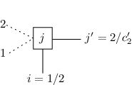
Figure 9: The pair of configurations after the colour of site j′j^{\prime} has been assigned during the first step of the coupling.
Refer to caption

We make the following observations about the resulting conditional distributions D1|j′=2D_{1}\mid j^{\prime}=2 and D2|j′=c2′D_{2}\mid j^{\prime}=c_{2}^{\prime}.

  • •

    The colour 22 is not valid for jj in either distribution D1|j′=2D_{1}\mid j^{\prime}=2 or D2|j′=c2′D_{2}\mid j^{\prime}=c_{2}^{\prime}.

  • •

    The colour 11 is not valid for jj in D1|j′=2D_{1}\mid j^{\prime}=2 but could be valid for jj in D2|j′=c2′D_{2}\mid j^{\prime}=c_{2}^{\prime}.

  • •

    The colour c2′c_{2}^{\prime} could be valid for jj in D1|j′=2D_{1}\mid j^{\prime}=2 but is not valid for jj in D2|j′=c2′D_{2}\mid j^{\prime}=c_{2}^{\prime}.

  • •

    For each c∈C∖{1,2,c2′}c\in C\setminus\{1,2,c_{2}^{\prime}\} the colour cc is valid for jj in D1|j′=2D_{1}\mid j^{\prime}=2 if and only if cc is valid for jj in D2|j′=c2′D_{2}\mid j^{\prime}=c_{2}^{\prime}.

These observations show that this case is a single-site disagreement sub problem and that there must be at least (q−3)−(Δ−2)=q−Δ−1(q-3)-(\Delta-2)=q-\Delta-1 colours that are valid for jj in both conditional distributions since jj has at most Δ−2\Delta-2 neighbours other than ii and j′j^{\prime}. Also, there is at most one colour which is valid for jj in one distribution but not in the other and since the coupling greedily maximises Hamming distance this implies

Pr(x′,y′)∈Ψk​(x,y)​(xj′≠yj′∣xj′′≠yj′′)≤1q−Δ.\textnormal{Pr}_{(x^{\prime},y^{\prime})\in\Psi_{k}(x,y)}(x_{j}^{\prime}\neq y_{j}^{\prime}\mid x_{j^{\prime}}^{\prime}\neq y_{j^{\prime}}^{\prime})\leq\frac{1}{q-\Delta}.

Now suppose that the same colour cc, say, is drawn for site j′j^{\prime} in both distributions during the first step of the coupling. Then the only site adjacent to ii that is coloured differently in the conditional distributions D1|j′=cD_{1}\mid j^{\prime}=c and D2|j′=cD_{2}\mid j^{\prime}=c is site ii, so using a similar reasoning to above we find

Pr(x′,y′)∈Ψk​(x,y)​(xj′≠yj′∣xj′′=yj′′)≤1q−Δ\textnormal{Pr}_{(x^{\prime},y^{\prime})\in\Psi_{k}(x,y)}(x_{j}^{\prime}\neq y_{j}^{\prime}\mid x_{j^{\prime}}^{\prime}=y_{j^{\prime}}^{\prime})\leq\frac{1}{q-\Delta}

and thus

ρi,jk\displaystyle\rho_{i,j}^{k} =max(x,y)∈Si⁡{Pr(x′,y′)∈Ψk​(x,y)​(xj′≠yj′)}\displaystyle=\max_{(x,y)\in S_{i}}\left\{\textnormal{Pr}_{(x^{\prime},y^{\prime})\in\Psi_{k}(x,y)}(x_{j}^{\prime}\neq y_{j}^{\prime})\right\}
=max(x,y)∈Si{Pr(x′,y′)∈Ψk​(x,y)(xj′≠yj′∣xj′′≠yj′′)Pr(x′,y′)∈Ψk​(x,y)(xj′′≠yj′′)\displaystyle=\max_{(x,y)\in S_{i}}\{\textnormal{Pr}_{(x^{\prime},y^{\prime})\in\Psi_{k}(x,y)}(x_{j}^{\prime}\neq y_{j}^{\prime}\mid x_{j^{\prime}}^{\prime}\neq y_{j^{\prime}}^{\prime})\textnormal{Pr}_{(x^{\prime},y^{\prime})\in\Psi_{k}(x,y)}(x_{j^{\prime}}^{\prime}\neq y_{j^{\prime}}^{\prime})
+Pr(x′,y′)∈Ψk​(x,y)(xj′≠yj′∣xj′′=yj′′)Pr(x′,y′)∈Ψk​(x,y)(xj′′=yj′′)}\displaystyle\quad+\textnormal{Pr}_{(x^{\prime},y^{\prime})\in\Psi_{k}(x,y)}(x_{j}^{\prime}\neq y_{j}^{\prime}\mid x_{j^{\prime}}^{\prime}=y_{j^{\prime}}^{\prime})\textnormal{Pr}_{(x^{\prime},y^{\prime})\in\Psi_{k}(x,y)}(x_{j^{\prime}}^{\prime}=y_{j^{\prime}}^{\prime})\}
≤max(x,y)∈Si⁡{1q−Δ​Pr(x′,y′)∈Ψk​(x,y)​(xj′′≠yj′′)+1q−Δ​Pr(x′,y′)∈Ψk​(x,y)​(xj′′=yj′′)}\displaystyle\leq\max_{(x,y)\in S_{i}}\left\{\frac{1}{q-\Delta}\textnormal{Pr}_{(x^{\prime},y^{\prime})\in\Psi_{k}(x,y)}(x_{j^{\prime}}^{\prime}\neq y_{j^{\prime}}^{\prime})+\frac{1}{q-\Delta}\textnormal{Pr}_{(x^{\prime},y^{\prime})\in\Psi_{k}(x,y)}(x_{j^{\prime}}^{\prime}=y_{j^{\prime}}^{\prime})\right\}
=1q−Δ​max(x,y)∈Si​{Pr(x′,y′)∈Ψk​(x,y)​(xj′′≠yj′′)+Pr(x′,y′)∈Ψk​(x,y)​(xj′′=yj′′)}=1q−Δ\displaystyle=\frac{1}{q-\Delta}\max_{(x,y)\in S_{i}}\left\{\textnormal{Pr}_{(x^{\prime},y^{\prime})\in\Psi_{k}(x,y)}(x_{j^{\prime}}^{\prime}\neq y_{j^{\prime}}^{\prime})+\textnormal{Pr}_{(x^{\prime},y^{\prime})\in\Psi_{k}(x,y)}(x_{j^{\prime}}^{\prime}=y_{j^{\prime}}^{\prime})\right\}=\frac{1}{q-\Delta}

which completes the proof. ∎

Details of case 4. (Repeated in Figure 10)

Figure 10: Case 4. Both sites in Θk\Theta_{k} are adjacent to ii. One of the sites in Θk\Theta_{k} is adjacent to at least one site, other than ii, coloured 1 and no sites that are coloured 2. Let this site be labeled j′j^{\prime}. The other site in Θk\Theta_{k}, labeled jj, is adjacent to at least one site other than ii coloured 2 and no sites coloured 1.
Refer to caption

We assume without loss of generality that d1≥d2d_{1}\geq d_{2} and construct the coupling Ψk​(x,y)\Psi_{k}(x,y) of D1D_{1} and D2D_{2} as follows. For each valid choice of the form c1​c2c_{1}c_{2} for D1D_{1} where c1≠1c_{1}\neq 1 and c2≠2c_{2}\neq 2 Lemma 9 guarantees that c1​c2c_{1}c_{2} is also valid for D2D_{2} so we construct Ψk​(x,y)\Psi_{k}(x,y) such that

Pr(x′,y′)∈Ψk​(x,y)​(x′=y′=c1​c2)=\displaystyle\textnormal{Pr}_{(x^{\prime},y^{\prime})\in\Psi_{k}(x,y)}(x^{\prime}=y^{\prime}=c_{1}c_{2})= 1d1.\displaystyle\frac{1}{d_{1}}.

This leaves the set Z1={c1​2∣c1​2​ valid in ​D1}Z_{1}=\{c_{1}2\mid c_{1}2\textnormal{ valid in }D_{1}\} of valid choices for D1D_{1} and Z2={1​c2∣1​c2​ valid in ​D2}⊆D2Z_{2}=\{1c_{2}\mid 1c_{2}\textnormal{ valid in }D_{2}\}\subseteq D_{2} for D2D_{2}. Observe that z1≥z2z_{1}\geq z_{2} where z1z_{1} and z2z_{2} denote the size of Z1Z_{1} and Z2Z_{2} respectively. Let Z1​(t)Z_{1}(t) denote the tt-th element of Z1Z_{1} and similarly for Z2Z_{2}. Then for 1≤t≤z21\leq t\leq z_{2} let

Pr(x′,y′)∈Ψk​(x,y)​(x′=Z1​(t),y′=Z2​(t))=1d1\textnormal{Pr}_{(x^{\prime},y^{\prime})\in\Psi_{k}(x,y)}(x^{\prime}=Z_{1}(t),y^{\prime}=Z_{2}(t))=\frac{1}{d_{1}}

and for each pair z2+1≤t≤z2z_{2}+1\leq t\leq z_{2} and h∈D2h\in D_{2} let

Pr(x′,y′)∈Ψk​(x,y)​(x′=Z1​(t),y′=h)=1d1​d2.\textnormal{Pr}_{(x^{\prime},y^{\prime})\in\Psi_{k}(x,y)}(x^{\prime}=Z_{1}(t),y^{\prime}=h)=\frac{1}{d_{1}d_{2}}.

It is easy to verify that each valid colouring has the correct weight in Ψk​(x,y)\Psi_{k}(x,y) so this completes the coupling.

Lemma 16.

Let jj and j′j^{\prime} be the endpoints of an edge Θk\Theta_{k} and suppose that {i,j}∈E⁡(G)\{i,j\}\in E(G) and {i,j′}∈E⁡(G)\{i,j^{\prime}\}\in E(G). If 11 is valid for jj in D2D_{2}, 11 is not valid for j′j^{\prime} in D2D_{2} and 22 is not valid for jj in D1D_{1} then

ρi,jk≤ρi,j′k≤1q−Δ.\rho_{i,j}^{k}\leq\rho_{i,j^{\prime}}^{k}\leq\frac{1}{q-\Delta}.
Proof.

This is case 4 of the coupling. Let s=∑cd2,j=c−d2,j=1s=\sum_{c}d_{2,j=c}-d_{2,j=1} be the number of valid choices for D2D_{2} other than choices of the form 1​c21c_{2}. Observe that d2=s+d1,j′=2d_{2}=s+d_{1,j^{\prime}=2} and note that d1,j′=2≥d2,j=1d_{1,j^{\prime}=2}\geq d_{2,j=1} since we have assumed d1≥d2d_{1}\geq d_{2} in the construction of the coupling. At least one neighbour, other than ii, of j′j^{\prime} on the boundary of Θk\Theta_{k} is coloured 1 in D1D_{1} and we get the following lower-bound on d2,j=1d_{2,j=1} since all other neighbours of j′j^{\prime} may be assigned a different colour

q−Δ+1≤d2,j=1.q-\Delta+1\leq d_{2,j=1}.

We bound ss using the same argument as in the proof of Lemma 15 and get

d1,j′=2​(d2,j=1−1)≤s.d_{1,j^{\prime}=2}(d_{2,j=1}-1)\leq s.

Since 22 is not valid for jj in D1D_{1} the first d2,j=1d_{2,j=1} choices of the form c1​2c_{1}2 for D1D_{1} are matched with some choice of the form 1​c11c_{1} for D2D_{2} with probability 1/d11/d_{1} resulting in a different colour being assigned to both sites jj and j′j^{\prime} in each distribution. Each of the d1,j′=2−d2,j=1d_{1,j^{\prime}=2}-d_{2,j=1} remaining valid choices for D1D_{1} is matched with each valid choice for D2D_{2} with probability 1d1​d2\frac{1}{d_{1}d_{2}} resulting in a disagreement at j′j^{\prime} (since 22 is not valid for j′j^{\prime} in D2D_{2}) and potentially also at at jj so ρi,jk≤ρi,j′k\rho_{i,j}^{k}\leq\rho_{i,j^{\prime}}^{k}. Hence the probability of making a choice of the form c1​2c_{1}2 for D1D_{1}

Pr(x′,y′)∈Ψk​(x,y)​(xj′′=2)=d2,j=1d1+∑h∈D2d1,j′=2−d2,j=1d1​d2=d1,j′=2d1\textnormal{Pr}_{(x^{\prime},y^{\prime})\in\Psi_{k}(x,y)}(x_{j^{\prime}}^{\prime}=2)=\frac{d_{2,j=1}}{d_{1}}+\sum_{h\in D_{2}}\frac{d_{1,j^{\prime}=2}-d_{2,j=1}}{d_{1}d_{2}}=\frac{d_{1,j^{\prime}=2}}{d_{1}}

is an upper bound on the disagreement probabilities at both sites jj and j′j^{\prime}. Using the lower bounds on ss and d2,j=1d_{2,j=1} we have

ρi,jk≤ρi,j′k≤d1,j′=2d1=d1,j′=2d1,j′=2+s≤d1,j′=2d1,j′=2+(d2,j=1−1)​d1,j′=2≤1q−Δ\rho_{i,j}^{k}\leq\rho_{i,j^{\prime}}^{k}\leq\frac{d_{1,j^{\prime}=2}}{d_{1}}=\frac{d_{1,j^{\prime}=2}}{d_{1,j^{\prime}=2}+s}\leq\frac{d_{1,j^{\prime}=2}}{d_{1,j^{\prime}=2}+(d_{2,j=1}-1)d_{1,j^{\prime}=2}}\leq\frac{1}{q-\Delta}

which completes the proof. ∎

Details of case 5. (Repeated in Figure 11)

Figure 11: Case 5. Both sites in Θk\Theta_{k} are adjacent to ii and at least one site, other than ii coloured 1. The labeling of the sites in Θk\Theta_{k} is arbitrary.
Refer to caption

First observe that 11 is not valid for both jj and j′j^{\prime} in either distribution D1D_{1} or D2D_{2} so d1=d2+d1,j=2+d1,j′=2≥d2d_{1}=d_{2}+d_{1,j=2}+d_{1,j^{\prime}=2}\geq d_{2} by Lemma 9, since any choice valid for D2D_{2} does not assign colour 22 to any site in Θk\Theta_{k}. Let Z1Z_{1} and Z2Z_{2} be the sets of colourings valid for D1D_{1} and D2D_{2} respectively. We define the following mutually exclusive subsets of Z1Z_{1}. Zj={2​c2∣2​c2∈Z1}Z_{j}=\{2c_{2}\mid 2c_{2}\in Z_{1}\}, Zj′={c1​2∣c1​2∈Z1}Z_{j^{\prime}}=\{c_{1}2\mid c_{1}2\in Z_{1}\} and Z=Z1∖(Zj∪Zj′)=Z2Z=Z_{1}\setminus(Z_{j}\cup Z_{j^{\prime}})=Z_{2}. By construction, the union of these three subsets is Z1Z_{1} and note that the size of ZjZ_{j} is d1,j=2d_{1,j=2}, the size of Zj′Z_{j^{\prime}} is d1,j′=2d_{1,j^{\prime}=2} and the size of ZZ is d2d_{2}.

First we consider choices from ZZ for D1D_{1}. For each choice h∈Zh\in Z we have h∈Z2h\in Z_{2} by construction of ZZ and so we use the identity coupling and let

Pr(x′,y′)∈Ψk​(x,y)​(x′=y′=h)=1d1.\textnormal{Pr}_{(x^{\prime},y^{\prime})\in\Psi_{k}(x,y)}(x^{\prime}=y^{\prime}=h)=\frac{1}{d_{1}}.

We let the remainder of the coupling minimise Hamming distance. First consider the choices for D1D_{1} in ZjZ_{j}. We construct Ψk​(x,y)\Psi_{k}(x,y) such that it minimises Hamming distance and assigns probability 1/d11/d_{1} to each choice for D1D_{1} in ZjZ_{j} whilst ensuring that for each choice g∈Z2g\in Z_{2} for D2D_{2}

∑h∈ZjPr(x′,y′)∈Ψk​(x,y)​(x′=h,y′=g)=d1,j=2d1​d2.\sum_{h\in Z_{j}}\textnormal{Pr}_{(x^{\prime},y^{\prime})\in\Psi_{k}(x,y)}(x^{\prime}=h,y^{\prime}=g)=\frac{d_{1,j=2}}{d_{1}d_{2}}.

Similarly we assign probability 1/d11/d_{1} to each choice for D1D_{1} in Zj′Z_{j^{\prime}} whilst also requiring that for each choice g∈Z2g\in Z_{2} for D2D_{2}

∑h∈Zj′Pr(x′,y′)∈Ψk​(x,y)​(x′=h,y′=g)=d1,j′=2d1​d2.\sum_{h\in Z_{j^{\prime}}}\textnormal{Pr}_{(x^{\prime},y^{\prime})\in\Psi_{k}(x,y)}(x^{\prime}=h,y^{\prime}=g)=\frac{d_{1,j^{\prime}=2}}{d_{1}d_{2}}.

To see that this ensures that the coupling is fair observe that each choice h∈Z1h\in Z_{1} receives weight 1/d11/d_{1} and each choice g∈Z2g\in Z_{2} weight

1d1+d1,j=2d1​d2+d1,j′=2d1​d2=d2+d1,j=2+d1,j′=2d1​d2=1d2\frac{1}{d_{1}}+\frac{d_{1,j=2}}{d_{1}d_{2}}+\frac{d_{1,j^{\prime}=2}}{d_{1}d_{2}}=\frac{d_{2}+d_{1,j=2}+d_{1,j^{\prime}=2}}{d_{1}d_{2}}=\frac{1}{d_{2}}

since d2+d1,j=2+d1,j′=2=d1d_{2}+d_{1,j=2}+d_{1,j^{\prime}=2}=d_{1}.

Remark.

Note that a coupling satisfying these requirements always exists. We will not give the detailed construction of Ψk​(x,y)\Psi_{k}(x,y) here, but in the subsequent proof we will consider three cases. In the first two cases any coupling minimising Hamming distance will be sufficient to establish the required bounds on the influence of ii on jj. In the final case we will need a detailed construction of the coupling and so will provide it together with the proof for ease of reference.

Lemma 17.

Let jj and j′j^{\prime} be the endpoints of an edge Θk\Theta_{k} and suppose that {i,j}∈E⁡(G)\{i,j\}\in E(G) and {i,j′}∈E⁡(G)\{i,j^{\prime}\}\in E(G). If 11 is not valid for jj in D2D_{2} and 11 is not valid for j′j^{\prime} in D2D_{2} then

ρi,jk≤1q−Δ+1+1(q−Δ+1)2​ and ​ρi,j′k≤1q−Δ+1+1(q−Δ+1)2.\rho_{i,j}^{k}\leq\frac{1}{q-\Delta+1}+\frac{1}{(q-\Delta+1)^{2}}\textnormal{ and }\rho_{i,j^{\prime}}^{k}\leq\frac{1}{q-\Delta+1}+\frac{1}{(q-\Delta+1)^{2}}.
Proof.

This is case 5 of the coupling. We consider three separate cases. Firstly suppose that 22 is not valid for both jj and j′j^{\prime} in D1D_{1}. Then the only valid choices for D1D_{1} are of the form c1​c2c_{1}c_{2} where c1,c2∈C∖{1,2}c_{1},c_{2}\in C\setminus\{1,2\} and each such choice is also valid in D2D_{2} as observed in the construction of the coupling. The same colouring is selected for each distribution and hence

ρi,jk=0​ and ​ρi,j′k=0.\rho_{i,j}^{k}=0\textnormal{ and }\rho_{i,j^{\prime}}^{k}=0.

Next suppose that exactly one site in Θk\Theta_{k}, j′j^{\prime} say, is adjacent to some site coloured 22 in D1D_{1}. As in the previous case, each choice that is valid in both D1D_{1} and D2D_{2} is matched using the identity matching and does not cause a discrepancy at any site. However if a choice of the form 2​c2c is made for D1D_{1} then site jj will be coloured differently in each colouring drawn from Ψk​(x,y)\Psi_{k}(x,y) and the colour at site j′j^{\prime} may also be different so ρi,j′k≤ρi,jk\rho_{i,j^{\prime}}^{k}\leq\rho_{i,j}^{k}. Since all choices of the form c​2c2 are not valid for D1D_{1}, making a choice of the form 2​c2c for D1D_{1} is the only way to create a disagreement at any site in the coupling and so

ρi,j′k≤ρi,jk≤d1,j=2d1\rho_{i,j^{\prime}}^{k}\leq\rho_{i,j}^{k}\leq\frac{d_{1,j=2}}{d_{1}}

since d1,j=2d_{1,j=2} is the number of valid choices for D1D_{1} of the form 2​c2c. We need to establish a lower bound of d1d_{1} and observe that, for cc valid for jj in D1D_{1}, d1,j=2−1≤d1,j=cd_{1,j=2}-1\leq d_{1,j=c} by Lemma 13 (ii) since 22 is not valid for j′j^{\prime} in D1D_{1}. Let vv be the number of colours that are valid for site jj in D1D_{1}. Then vv is lower bounded by q−Δ+2≤vq-\Delta+2\leq v since at least two of the sites (including ii) adjacent to jj on the boundary of Θk\Theta_{k} are coloured 11 in D1D_{1}. Also, since at least one site (other than jj and ii) adjacent to j′j^{\prime} is coloured 11 and another is coloured 22 in D1D_{1}, we have q−Δ+2≤d1,j=2q-\Delta+2\leq d_{1,j=2}. Using the lower bounds on vv and d1,j=cd_{1,j=c} we have, letting JJ denote the set of colours other than 22 that are valid for jj in D1D_{1},

d1=∑cd1,j=c\displaystyle d_{1}=\sum_{c}d_{1,j=c} =d1,j=2+∑c∈Jd1,j=c≥d1,j=2+∑c∈J(d1,j=2−1)\displaystyle=d_{1,j=2}+\sum_{c\in J}d_{1,j=c}\geq d_{1,j=2}+\sum_{c\in J}(d_{1,j=2}-1)
≥(v−1)​(d1,j=2−1)+d1,j=2≥(q−Δ+2)​d1,j=2−(q−Δ+1)\displaystyle\geq(v-1)(d_{1,j=2}-1)+d_{1,j=2}\geq(q-\Delta+2)d_{1,j=2}-(q-\Delta+1)

and hence using the lower bound on d1,j=2d_{1,j=2}

1ρi,jk\displaystyle\frac{1}{\rho_{i,j}^{k}} ≥(q−Δ+2)​d1,j=2−(q−Δ+1)d1,j=2≥q−Δ+2−q−Δ+1q−Δ+2>q−Δ+1\displaystyle\geq\frac{(q-\Delta+2)d_{1,j=2}-(q-\Delta+1)}{d_{1,j=2}}\geq q-\Delta+2-\frac{q-\Delta+1}{q-\Delta+2}>q-\Delta+1

which gives the bounds required by the statement of the lemma.

Finally consider the case when the colour 22 is valid for both jj and j′j^{\prime} in D1D_{1}. In this case we will provide details of the construction of Ψk​(x,y)\Psi_{k}(x,y) when required. We begin by establishing some required bounds. Since 11 is not valid for j′j^{\prime} in D2D_{2} at least two neighbours of j′j^{\prime} (including ii) must be coloured 11 in D1D_{1} and the same applies to the neighbourhood of jj, so we get the following lower bounds on d1,j=2d_{1,j=2} and d1,j′=2d_{1,j^{\prime}=2}

q−Δ+1≤d1,j=2​ and ​q−Δ+1≤d1,j′=2.q-\Delta+1\leq d_{1,j=2}\textnormal{ and }q-\Delta+1\leq d_{1,j^{\prime}=2}.

We also require bounds on d2,j=cd_{2,j=c} and d2,j′=cd_{2,j^{\prime}=c} for other colours cc. Suppose that the choice c​c′cc^{\prime} is valid in D2D_{2} then, since c,c′∈C∖{1,2}c,c^{\prime}\in C\setminus\{1,2\}, c​c′cc^{\prime} is also valid for D1D_{1} by Lemma 9. Furthermore, the choice c​2c2 is valid in D1D_{1} (but not D2D_{2}) so d1,j=c−1=d2,j=cd_{1,j=c}-1=d_{2,j=c}. Lemma 13 (ii) guarantees that d1,j=2≤d1,j=c≤d1,j=2+1d_{1,j=2}\leq d_{1,j=c}\leq d_{1,j=2}+1 so

d1,j=2−1≤d2,j=c≤d1,j=2d_{1,j=2}-1\leq d_{2,j=c}\leq d_{1,j=2}

for any cc valid for jj in D1D_{1} and a similar argument gives the bound

d1,j′=2−1≤d2,j′=c≤d1,j′=cd_{1,j^{\prime}=2}-1\leq d_{2,j^{\prime}=c}\leq d_{1,j^{\prime}=c}

for any colour cc valid for j′j^{\prime} in D2D_{2}. Observe that exactly d1,j′=2d_{1,j^{\prime}=2} colours must be valid for site jj in D2D_{2} so using the stated bounds on d2,j=cd_{2,j=c} we have the following bounds on d2d_{2}

d1,j′=2​(d1,j=2−1)≤d2≤d1,j′=2​d1,j=2.d_{1,j^{\prime}=2}(d_{1,j=2}-1)\leq d_{2}\leq d_{1,j^{\prime}=2}d_{1,j=2}.

We bound the probability of disagreements at sites jj and j′j^{\prime} from choices made for D1D_{1}. From the coupling we again note that if a choice c1​c2c_{1}c_{2} where c1≠2c_{1}\neq 2 and c2≠2c_{2}\neq 2 is made for D1D_{1} then there will be no disagreements at any site in Θk\Theta_{k}.

Consider making a valid choice of the form 2​c2c for D1D_{1}. Firstly, such a choice for D1D_{1} will cause site jj to be coloured differently in any pair of colourings drawn from the coupling since 22 is not valid for jj in D2D_{2}. We construct Ψk​(x,y)\Psi_{k}(x,y) such that the choice 2​c2c for D1D_{1} is matched with a choice of the form c′​cc^{\prime}c for D2D_{2} as long as such a choice that has not exceeded it aggregated probability exists. Let JJ denote the set of choices of the form c′​cc^{\prime}c that are valid for D2D_{2} and note that the size of JJ is d2,j′=cd_{2,j^{\prime}=c}. The total aggregated weight of all choices of the form c′​cc^{\prime}c for D2D_{2} is

∑g∈J∑h∈Z1Pr(x′,y′)∈Ψk​(x,y)​(x′=h,y′=g)=∑g∈Jd1,j=2d1​d2=d2,j′=c​d1,j=2d1​d2\sum_{g\in J}\sum_{h\in Z_{1}}\textnormal{Pr}_{(x^{\prime},y^{\prime})\in\Psi_{k}(x,y)}(x^{\prime}=h,y^{\prime}=g)=\sum_{g\in J}\frac{d_{1,j=2}}{d_{1}d_{2}}=\frac{d_{2,j^{\prime}=c}d_{1,j=2}}{d_{1}d_{2}}

so as long as

1d1≤d2,j′=c​d1,j=2d1​d2\frac{1}{d_{1}}\leq\frac{d_{2,j^{\prime}=c}d_{1,j=2}}{d_{1}d_{2}}

there is enough probability available in Z2Z_{2} to match all the weight of the choice 2​c2c for D1D_{1} with a choice of the form c′​cc^{\prime}c for D2D_{2} and hence assigning the same colour, cc, to site j′j^{\prime} in any pair of colourings drawn from the coupling. If there is not enough unassigned weight available in Z2Z_{2} then the coupling will match at much probability as possible, d2,j′=c​d1,j=2d1​d2\frac{d_{2,j^{\prime}=c}d_{1,j=2}}{d_{1}d_{2}}, with choices of the form c′​cc^{\prime}c for Z2Z_{2} but the remaining probability will be matched with choices not assigning colour cc to site j′j^{\prime} in Z2Z_{2}. Hence we obtain the following probabilities conditioned on making a choice of the form 2​c2c for D1D_{1}.

Pr(x′,y′)∈Ψk​(x,y)​(xj′≠yj′∣x′=2​c)=1\textnormal{Pr}_{(x^{\prime},y^{\prime})\in\Psi_{k}(x,y)}(x_{j}^{\prime}\neq y_{j}^{\prime}\mid x^{\prime}=2c)=1

and

Pr(x′,y′)∈Ψk​(x,y)​(xj′′≠yj′′∣x′=2​c)\displaystyle\textnormal{Pr}_{(x^{\prime},y^{\prime})\in\Psi_{k}(x,y)}(x_{j^{\prime}}^{\prime}\neq y_{j^{\prime}}^{\prime}\mid x^{\prime}=2c) ≤max⁡(0,1−d2,j′=c​d1,j=2d2)\displaystyle\leq\max\left(0,1-\frac{d_{2,j^{\prime}=c}d_{1,j=2}}{d_{2}}\right)
≤max⁡(0,1−(d1,j′=2−1)​d1,j=2d1,j=2​d1,j′=2)\displaystyle\leq\max\left(0,1-\frac{(d_{1,j^{\prime}=2}-1)d_{1,j=2}}{d_{1,j=2}d_{1,j^{\prime}=2}}\right)
≤1d1,j′=2\displaystyle\leq\frac{1}{d_{1,j^{\prime}=2}}

using the bounds on d2d_{2} and d1,j′=cd_{1,j^{\prime}=c}. Lastly observe that there are d1,j=2d_{1,j=2} valid choices for D1D_{1} of the form 2​c2c so

∑cPr(x′,y′)∈Ψk​(x,y)​(x′=2​c)=d1,j=2d1=d1,j=2d1,j=2+d1,j′=2+d2.\sum_{c}\textnormal{Pr}_{(x^{\prime},y^{\prime})\in\Psi_{k}(x,y)}(x^{\prime}=2c)=\frac{d_{1,j=2}}{d_{1}}=\frac{d_{1,j=2}}{d_{1,j=2}+d_{1,j^{\prime}=2}+d_{2}}.

Also consider making a valid choice of the form c​2c2 for D1D_{1}. This case is symmetric to the construction above, but we include it for completeness. A choice of the form c​2c2 for D1D_{1} will cause site j′j^{\prime} to be coloured differently in any pair of colourings drawn from the coupling since 22 is not valid for j′j^{\prime} in D2D_{2}. We hence construct Ψk​(x,y)\Psi_{k}(x,y) such that it matches the choice c​2c2 for D1D_{1} with a choice of the form c​c′cc^{\prime} for D2D_{2} as long as such a choice that has not exceeded it aggregated probability exists. Let J′J^{\prime} denote the set of choices of the form c​c′cc^{\prime} that are valid for D2D_{2} and note that the size of J′J^{\prime} is d2,j=cd_{2,j=c}. The total aggregated weight of all choices of the form c​c′cc^{\prime} for D2D_{2} is

∑g∈J′∑h∈Z1Pr(x′,y′)∈Ψk​(x,y)​(x′=h,y′=g)=∑g∈Jd1,j′=2d1​d2=d2,j=c​d1,j′=2d1​d2\sum_{g\in J^{\prime}}\sum_{h\in Z_{1}}\textnormal{Pr}_{(x^{\prime},y^{\prime})\in\Psi_{k}(x,y)}(x^{\prime}=h,y^{\prime}=g)=\sum_{g\in J}\frac{d_{1,j^{\prime}=2}}{d_{1}d_{2}}=\frac{d_{2,j=c}d_{1,j^{\prime}=2}}{d_{1}d_{2}}

so as long as

1d1≤d2,j=c​d1,j′=2d1​d2\frac{1}{d_{1}}\leq\frac{d_{2,j=c}d_{1,j^{\prime}=2}}{d_{1}d_{2}}

there is enough weight available in Z2Z_{2} to match all the weight of the choice c​2c2 for D1D_{1} with a choice of the form c​c′cc^{\prime} for D2D_{2} and hence assigning the same colour, cc, to site jj in any pair of colourings drawn from the coupling. If there is not enough unassigned weight available in Z2Z_{2} then the coupling will match at much weight as possible, d2,j=c​d1,j′=2d1​d2\frac{d_{2,j=c}d_{1,j^{\prime}=2}}{d_{1}d_{2}}, with choices of the form c​c′cc^{\prime} for Z2Z_{2} but the remaining weight will be matched with choices not assigning colour cc to site jj in Z2Z_{2}. Hence we obtain the following probabilities conditioned on making a choice of the form c​2c2 for D1D_{1}

Pr(x′,y′)∈Ψk​(x,y)​(xj′≠yj′∣x′=c​2)\displaystyle\textnormal{Pr}_{(x^{\prime},y^{\prime})\in\Psi_{k}(x,y)}(x_{j}^{\prime}\neq y_{j}^{\prime}\mid x^{\prime}=c2) ≤max⁡(0,1−d2,j=c​d1,j′=2d2)\displaystyle\leq\max\left(0,1-\frac{d_{2,j=c}d_{1,j^{\prime}=2}}{d_{2}}\right)
≤max⁡(0,1−d1,j′=2​(d1,j=2−1)d1,j=2​d1,j′=2)\displaystyle\leq\max\left(0,1-\frac{d_{1,j^{\prime}=2}(d_{1,j=2}-1)}{d_{1,j=2}d_{1,j^{\prime}=2}}\right)
≤1d1,j=2\displaystyle\leq\frac{1}{d_{1,j=2}}

using the bounds on d2d_{2} and d1,j=cd_{1,j=c}, and as before we also have

Pr(x′,y′)∈Ψk​(x,y)​(xj′′≠yj′′∣x′=c​2)=1​ and ​∑cPr(x′,y′)∈Ψk​(x,y)​(x′=c​2)=d1,j′=2d1,j=2+d1,j′=2+d2.\textnormal{Pr}_{(x^{\prime},y^{\prime})\in\Psi_{k}(x,y)}(x_{j^{\prime}}^{\prime}\neq y_{j^{\prime}}^{\prime}\mid x^{\prime}=c2)=1\mbox{ and }\sum_{c}\textnormal{Pr}_{(x^{\prime},y^{\prime})\in\Psi_{k}(x,y)}(x^{\prime}=c2)=\frac{d_{1,j^{\prime}=2}}{d_{1,j=2}+d_{1,j^{\prime}=2}+d_{2}}.

Using the conditional probabilities and the bounds on d2d_{2}, d1,j=2d_{1,j=2} and d1,j′=2d_{1,j^{\prime}=2} we find

ρi,jk\displaystyle\rho_{i,j}^{k} =max(x,y)∈Si⁡{Pr(x′,y′)∈Ψk​(x,y)​(xj′≠yj′)}\displaystyle=\max_{(x,y)\in S_{i}}\left\{\textnormal{Pr}_{(x^{\prime},y^{\prime})\in\Psi_{k}(x,y)}(x_{j}^{\prime}\neq y_{j}^{\prime})\right\}
=max(x,y)∈Si{∑cPr(x′,y′)∈Ψk​(x,y)(xj′≠yj′∣x′=2c)Pr(x′,y′)∈Ψk​(x,y)(x′=2c)\displaystyle=\max_{(x,y)\in S_{i}}\Big\{\sum_{c}\textnormal{Pr}_{(x^{\prime},y^{\prime})\in\Psi_{k}(x,y)}(x_{j}^{\prime}\neq y_{j}^{\prime}\mid x^{\prime}=2c)\textnormal{Pr}_{(x^{\prime},y^{\prime})\in\Psi_{k}(x,y)}(x^{\prime}=2c)
+∑cPr(x′,y′)∈Ψk​(x,y)(xj′≠yj′∣x′=c2)Pr(x′,y′)∈Ψk​(x,y)(x′=c2)}\displaystyle\quad+\sum_{c}\textnormal{Pr}_{(x^{\prime},y^{\prime})\in\Psi_{k}(x,y)}(x_{j}^{\prime}\neq y_{j}^{\prime}\mid x^{\prime}=c2)\textnormal{Pr}_{(x^{\prime},y^{\prime})\in\Psi_{k}(x,y)}(x^{\prime}=c2)\Big\}
≤max(x,y)∈Si⁡{∑c[Pr(x′,y′)∈Ψk​(x,y)​(x′=2​c)+Pr(x′,y′)∈Ψk​(x,y)​(x′=c​2)​1d1,j=2]}\displaystyle\leq\max_{(x,y)\in S_{i}}\left\{\sum_{c}\left[\textnormal{Pr}_{(x^{\prime},y^{\prime})\in\Psi_{k}(x,y)}(x^{\prime}=2c)+\textnormal{Pr}_{(x^{\prime},y^{\prime})\in\Psi_{k}(x,y)}(x^{\prime}=c2)\frac{1}{d_{1,j=2}}\right]\right\}
≤max(x,y)∈Si⁡{d1,j=2d1,j=2+d1,j′=2+d2+∑cPr(x′,y′)∈Ψk​(x,y)​(x′=c​2)​1d1,j=2}\displaystyle\leq\max_{(x,y)\in S_{i}}\left\{\frac{d_{1,j=2}}{d_{1,j=2}+d_{1,j^{\prime}=2}+d_{2}}+\sum_{c}\textnormal{Pr}_{(x^{\prime},y^{\prime})\in\Psi_{k}(x,y)}(x^{\prime}=c2)\frac{1}{d_{1,j=2}}\right\}
≤max(x,y)∈Si⁡{d1,j=2d1,j=2​(1+d1,j′=2)+d1,j′=2d1,j=2+d1,j′=2+d2​1d1,j=2}\displaystyle\leq\max_{(x,y)\in S_{i}}\left\{\frac{d_{1,j=2}}{d_{1,j=2}(1+d_{1,j^{\prime}=2})}+\frac{d_{1,j^{\prime}=2}}{d_{1,j=2}+d_{1,j^{\prime}=2}+d_{2}}\frac{1}{d_{1,j=2}}\right\}
≤max(x,y)∈Si⁡{11+d1,j′=2+d1,j′=2d1,j=2​(1+d1,j′=2)​1d1,j=2}\displaystyle\leq\max_{(x,y)\in S_{i}}\left\{\frac{1}{1+d_{1,j^{\prime}=2}}+\frac{d_{1,j^{\prime}=2}}{d_{1,j=2}(1+d_{1,j^{\prime}=2})}\frac{1}{d_{1,j=2}}\right\}
≤1q−Δ+2+1(q−Δ+1)2\displaystyle\leq\frac{1}{q-\Delta+2}+\frac{1}{(q-\Delta+1)^{2}}

and again by symmetry

ρi,j′k\displaystyle\rho_{i,j^{\prime}}^{k} =max(x,y)∈Si{Pr(x′,y′)∈Ψk​(x,y)(xj′′≠yj′′}\displaystyle=\max_{(x,y)\in S_{i}}\left\{\textnormal{Pr}_{(x^{\prime},y^{\prime})\in\Psi_{k}(x,y)}(x_{j^{\prime}}^{\prime}\neq y_{j^{\prime}}^{\prime}\right\}
=max(x,y)∈Si{∑cPr(x′,y′)∈Ψk​(x,y)(xj′′≠yj′′∣x′=2c)Pr(x′,y′)∈Ψk​(x,y)(x′=2c)\displaystyle=\max_{(x,y)\in S_{i}}\Big\{\sum_{c}\textnormal{Pr}_{(x^{\prime},y^{\prime})\in\Psi_{k}(x,y)}(x_{j^{\prime}}^{\prime}\neq y_{j^{\prime}}^{\prime}\mid x^{\prime}=2c)\textnormal{Pr}_{(x^{\prime},y^{\prime})\in\Psi_{k}(x,y)}(x^{\prime}=2c)
+∑cPr(x′,y′)∈Ψk​(x,y)(xj′′≠yj′′∣x′=c2)Pr(x′,y′)∈Ψk​(x,y)(x′=c2)}\displaystyle\quad+\sum_{c}\textnormal{Pr}_{(x^{\prime},y^{\prime})\in\Psi_{k}(x,y)}(x_{j^{\prime}}^{\prime}\neq y_{j^{\prime}}^{\prime}\mid x^{\prime}=c2)\textnormal{Pr}_{(x^{\prime},y^{\prime})\in\Psi_{k}(x,y)}(x^{\prime}=c2)\Big\}
≤max(x,y)∈Si⁡{∑c[Pr(x′,y′)∈Ψk​(x,y)​(x′=2​c)+Pr(x′,y′)∈Ψk​(x,y)​(x′=c​2)​1d1,j′=2]}\displaystyle\leq\max_{(x,y)\in S_{i}}\left\{\sum_{c}\left[\textnormal{Pr}_{(x^{\prime},y^{\prime})\in\Psi_{k}(x,y)}(x^{\prime}=2c)+\textnormal{Pr}_{(x^{\prime},y^{\prime})\in\Psi_{k}(x,y)}(x^{\prime}=c2)\frac{1}{d_{1,j^{\prime}=2}}\right]\right\}
≤max(x,y)∈Si⁡{d1,j′=2d1,j=2+d1,j′=2+d2+∑cPr(x′,y′)∈Ψk​(x,y)​(x′=c​2)​1d1,j′=2}\displaystyle\leq\max_{(x,y)\in S_{i}}\left\{\frac{d_{1,j^{\prime}=2}}{d_{1,j=2}+d_{1,j^{\prime}=2}+d_{2}}+\sum_{c}\textnormal{Pr}_{(x^{\prime},y^{\prime})\in\Psi_{k}(x,y)}(x^{\prime}=c2)\frac{1}{d_{1,j^{\prime}=2}}\right\}
≤max(x,y)∈Si⁡{d1,j′=2d1,j=2​(1+d1,j′=2)+d1,j=2d1,j=2+d1,j′=2+d2​1d1,j′=2}\displaystyle\leq\max_{(x,y)\in S_{i}}\left\{\frac{d_{1,j^{\prime}=2}}{d_{1,j=2}(1+d_{1,j^{\prime}=2})}+\frac{d_{1,j=2}}{d_{1,j=2}+d_{1,j^{\prime}=2}+d_{2}}\frac{1}{d_{1,j^{\prime}=2}}\right\}
≤max(x,y)∈Si⁡{11+d1,j=​2+d1,j=2d1,j=2​(1+d1,j′=2)​1d1,j′=2}\displaystyle\leq\max_{(x,y)\in S_{i}}\left\{\frac{1}{1+d_{1,j^{=}2}}+\frac{d_{1,j=2}}{d_{1,j=2}(1+d_{1,j^{\prime}=2})}\frac{1}{d_{1,j^{\prime}=2}}\right\}
≤1q−Δ+1+1(q−Δ+1)2\displaystyle\leq\frac{1}{q-\Delta+1}+\frac{1}{(q-\Delta+1)^{2}}

which implies the statement of the lemma. ∎

This completes the cases of the coupling and we combine the obtained bounds on ρi,jk\rho_{i,j}^{k} and ρi,j′k\rho_{i,j^{\prime}}^{k} in the following corollary of Lemmas 14, 15, 16 and 17 which we use in establishing the mixing time of ℳedge\mathcal{M}_{\textnormal{edge}}.

Corollary 18.

Let jj and j′j^{\prime} be the endpoints of an edge Θk\Theta_{k}. If {i,j}∈E⁡(G)\{i,j\}\in E(G) and {i,j′}∈E⁡(G)\{i,j^{\prime}\}\in E(G) then

ρi,jk≤1q−Δ+1(q−Δ)2​ and ​ρi,j′k≤1q−Δ+1(q−Δ)2.\rho_{i,j}^{k}\leq\frac{1}{q-\Delta}+\frac{1}{(q-\Delta)^{2}}\textnormal{ and }\rho_{i,j^{\prime}}^{k}\leq\frac{1}{q-\Delta}+\frac{1}{(q-\Delta)^{2}}.
Remark.

Note that the bound in Corollary 18 is never tight. This bound could be improved, however this would only allow us to beat the 2​Δ2\Delta bound for special graphs since the bounds in Lemma 10 are tight.

We are now ready to present a proof of Theorem 3.
Theorem 3. Let GG be a graph with maximum vertex-degree Δ\Delta. If q≥2​Δq\geq 2\Delta then

Mix​(ℳedge,ε)≤Δ2​log⁡(n​ε−1).\textnormal{Mix}(\mathcal{M}_{\textnormal{edge}},\varepsilon)\leq\Delta^{2}\log(n\varepsilon^{-1}).
Proof.

Let jj and j′j^{\prime} be the endpoints of an edge represented by a block Θk\Theta_{k}. Let αj=∑iρi,jk\alpha_{j}=\sum_{i}\rho_{i,j}^{k} be the influence on site jj and αj′=∑iρi,j′k\alpha_{j^{\prime}}=\sum_{i}\rho_{i,j^{\prime}}^{k} then influence on j′j^{\prime}. Then α=max⁡(αj,αj′)\alpha=\max(\alpha_{j},\alpha_{j^{\prime}}). Suppose that Θk\Theta_{k} is adjacent to tt triangles, that is there are tt sites i1,…,iti_{1},\dots,i_{t} such that {i,j}∈E⁡(G)\{i,j\}\in E(G) and {i,j′}∈E⁡(G)\{i,j^{\prime}\}\in E(G) for each i∈{i1,…,it}i\in\{i_{1},\dots,i_{t}\}. Note that 0≤t≤Δ−10\leq t\leq\Delta-1. There are at most Δ−1−t\Delta-1-t sites adjacent to jj that are not adjacent to j′j^{\prime} and at most Δ−1−t\Delta-1-t sites adjacent to j′j^{\prime} that are not adjacent to jj. From Lemma 10 a site adjacent only to jj will emit an influence of at most 1q−Δ\frac{1}{q-\Delta} on site jj and Lemma 10 also guarantees that a site only adjacent to j′j^{\prime} can emit an influence at most 1(q−Δ)2\frac{1}{(q-\Delta)^{2}} on site jj. Corollary 18 says that a site adjacent to both jj and j′j^{\prime} can emit an influence of at most 1q−Δ+1(q−Δ)2\frac{1}{q-\Delta}+\frac{1}{(q-\Delta)^{2}} on site jj and hence

αj\displaystyle\alpha_{j} ≤t⁡(1q−Δ+1(q−Δ)2)+(Δ−1−t)​(1q−Δ)+(Δ−1−t)​(1(q−Δ)2)\displaystyle\leq t\left(\frac{1}{q-\Delta}+\frac{1}{(q-\Delta)^{2}}\right)+(\Delta-1-t)\left(\frac{1}{q-\Delta}\right)+(\Delta-1-t)\left(\frac{1}{(q-\Delta)^{2}}\right)
=Δ−1q−Δ+Δ−1(q−Δ)2\displaystyle=\frac{\Delta-1}{q-\Delta}+\frac{\Delta-1}{(q-\Delta)^{2}}

and similarly by considering the influence on site j′j^{\prime} we find that

αj′≤Δ−1q−Δ+Δ−1(q−Δ)2.\alpha_{j^{\prime}}\leq\frac{\Delta-1}{q-\Delta}+\frac{\Delta-1}{(q-\Delta)^{2}}.

Then using our assumption that q≥2​Δq\geq 2\Delta we have

α=max⁡(αj,αj′)≤Δ−1q−Δ+Δ−1(q−Δ)2≤Δ−1Δ+Δ−1Δ2=Δ2−1Δ2=1−1Δ2<1\alpha=\max(\alpha_{j},\alpha_{j^{\prime}})\leq\frac{\Delta-1}{q-\Delta}+\frac{\Delta-1}{(q-\Delta)^{2}}\leq\frac{\Delta-1}{\Delta}+\frac{\Delta-1}{\Delta^{2}}=\frac{\Delta^{2}-1}{\Delta^{2}}=1-\frac{1}{\Delta^{2}}<1

and we obtain the stated bound on the mixing time by applying Theorem 2. ∎

4 Application: Colouring a Tree

This section contains the proof of Theorem 4 which improves the least number of colours required for mixing of systematic scan on a tree for individual values of Δ\Delta. Recall the definition of the systematic scan ℳtree\mathcal{M}_{\textnormal{tree}} where the set of blocks Θ\Theta is defined as follows. Let the block Θk\Theta_{k} contain a site rr along with all sites below rr in the tree that are at most h−1h-1 edges away from rr. We call hh the height of the blocks and hh is defined for each Δ\Delta in Table 1. The set of blocks Θ\Theta covers the sites of the tree and we construct Θ\Theta such that no block has height less than hh. P[k]P^{[k]} is the transition matrix for performing a heat-bath move on block Θk\Theta_{k} and hence P[k]​(x)P^{[k]}(x) is the uniform distribution on the set of configurations that agree with xx off Θk\Theta_{k} and where no edge incident to a site in Θk\Theta_{k} is monochromatic. The transition matrix of the Markov chain ℳtree\mathcal{M}_{\textnormal{tree}} is Πk=1m​P[k]\Pi_{k=1}^{m}P^{[k]} where mm is the number of blocks.

We will use standard terminology when discussing the structure of the tree. In particular will say that a site ii is a descendant of a site jj (or jj is a predecessor of ii) if jj is on the simple path from the root of the tree to ii. We will call a site jj a child of a site ii (or ii is the parent of jj) if ii and jj are adjacent and jj is a descendant of ii. Finally Nk​(j)={i∈∂Θk∣i​ is a descendant of ​j}N_{k}(j)=\{i\in\partial\Theta_{k}\mid i\textnormal{ is a descendant of }j\} is the set of descendants of jj on the boundary of Θk\Theta_{k}.

Let (x,y)∈Si(x,y)\in S_{i} where ii is on the boundary of some block Θk\Theta_{k}. The following lemma will provide upper bounds on the probability of disagreement at any site in the block.

Lemma 19.

Let (x,y)∈Si(x,y)\in S_{i} and suppose that ii is adjacent to exactly one site in a block Θk\Theta_{k}. Then there exists a coupling ψ\psi of D1=P[k]​(x)D_{1}=P^{[k]}(x) and D2=P[k]​(y)D_{2}=P^{[k]}(y) in which

Pr(x′,y′)∈ψ​(xj′≠yj′)≤1(q−Δ)d⁡(i,j)\textnormal{Pr}_{(x^{\prime},y^{\prime})\in\psi}(x_{j}^{\prime}\neq y_{j}^{\prime})\leq\frac{1}{(q-\Delta)^{d(i,j)}}

for all j∈Θkj\in\Theta_{k} where d⁡(i,j)d(i,j) is the edge distance from ii to jj.

Proof.

We construct a coupling ψ\psi of D1D_{1} and D2D_{2} based on the recursive coupling defined in Goldberg et al. [10]. The following definitions are based on Figure 12.

Figure 12: The region defined in a boundary pair and the construction of the subtrees.
Refer to caption

Let R⊆VR\subseteq V be a set of sites. Also let (X,X′)(X,X^{\prime}) be a pair of colourings of the sites on the boundary of RR (recall that the boundary of RR is the set of sites that are not included in RR but are adjacent to some site in RR) which use the same colour for every site, except for one site uu which is coloured ll in XX and l′l^{\prime} in X′X^{\prime}. We then say that A⁡(R,(X,X′),u,(l,l′))A(R,(X,X^{\prime}),u,(l,l^{\prime})) is a boundary pair. For a boundary pair A⁡(R,(X,X′),u,(l,l′))A(R,(X,X^{\prime}),u,(l,l^{\prime})) we let v∈Rv\in R be the site in RR that is adjacent to uu. We think of vv as the root of RR and note that we may need to turn the original tree “upside down” in order to achieve this, however the meaning should be clear. We then label the children (in RR) of vv as v1,…,vdv_{1},\dots,v_{d} and let T={R1,…,Rd}T=\{R_{1},\dots,R_{d}\} be set the of dd subtrees of RR that do not contain site vv, that is for Rk∈TR_{k}\in T we define Rk={j∈R∣j=vk​ or ​j​ is a descendant of ​vk}R_{k}=\{j\in R\mid j=v_{k}\mbox{ or }j\mbox{ is a descendant of }v_{k}\}. Finally let DD and D′D^{\prime} be the uniform distributions on colourings of RR consistent with the boundary colourings XX and X′X^{\prime} respectively and let D⁡(v)D(v) (respectively D′​(v)D^{\prime}(v)) be the uniform distribution on the color at site vv induced by DD (respectively D′D^{\prime}). Then ΨR\Psi_{R} is the recursive coupling of DD and D′D^{\prime} summarised as follows.

  1. 1.

    If l=l′l=l^{\prime} then the distributions DD and D′D^{\prime} are the same and we use the identity coupling, in which the same colouring is used in both copies. Otherwise we couple D⁡(v)D(v) and D′​(v)D^{\prime}(v) greedily to maximise the probability of assigning the same colour to site vv in both distributions. If RR consists of a single site then this completes the coupling.

  2. 2.

    Suppose that the pair of colours (c,c′)(c,c^{\prime}) were drawn for vv in the coupling from step 1. For each subtree R′∈{R1,…​Rd}R^{\prime}\in\{R_{1},\dots R_{d}\} we have a well defined boundary pair A⁡(R′,(XR′,XR′′),v,(c,c′))A(R^{\prime},(X_{R^{\prime}},X_{R^{\prime}}^{\prime}),v,(c,c^{\prime})) where XR′X_{R^{\prime}} is the boundary colouring XX restricted to the sites on the boundary of R′R^{\prime}. For each pair of colours (c,c′)(c,c^{\prime}) and R′∈TR^{\prime}\in T we recursively construct a coupling ΨR′​(c,c′)\Psi_{R^{\prime}}(c,c^{\prime}) of the distributions induced by the boundary pair A⁡(R′,(XR′,XR′′),v,(c,c′))A(R^{\prime},(X_{R^{\prime}},X_{R^{\prime}}^{\prime}),v,(c,c^{\prime})).

Initially we let the boundary pair be A⁡(R=Θk,(X=x,Y=y),u=i,(l=xi,l′=yi))A(R=\Theta_{k},(X=x,Y=y),u=i,(l=x_{i},l^{\prime}=y_{i})) and our coupling ψ\psi of D1D_{1} and D2D_{2} is thus the recursive coupling ΨΘk\Psi_{\Theta_{k}} constructed above.

We prove the statement of the lemma by induction on d⁡(i,j)d(i,j). The base case is d⁡(i,j)=1d(i,j)=1. Applying Lemma 13 from Goldberg et al. [10] we can upper bound the probability of xj′≠yj′x_{j}^{\prime}\neq y_{j}^{\prime} where (x′,y′)(x^{\prime},y^{\prime}) is drawn from ψ\psi by assigning the worst possible colouring to neighbours of jj in Θk\Theta_{k}. Site jj has at most Δ−1\Delta-1 neighbours (other than ii) so there are at least q−Δq-\Delta colours available for jj in both distributions. There is also at most one colour which is valid for jj in xx but not in yy (and vice versa) so

Pr(x′,y′)∈ψ​(xj′≠yj′)≤1q−Δ.\textnormal{Pr}_{(x^{\prime},y^{\prime})\in\psi}(x_{j}^{\prime}\neq y_{j}^{\prime})\leq\frac{1}{q-\Delta}.

Now let R′R^{\prime} be the subtree of Θk\Theta_{k} containing site jj and let vv be the site in Θk\Theta_{k} adjacent to ii. Assume that for d⁡(v,j)=d⁡(i,j)−1d(v,j)=d(i,j)-1

Pr(x′,y′)∈ΨR′​(c,c′)​(xj′≠yj′)≤1(q−Δ)d⁡(v,j).\textnormal{Pr}_{(x^{\prime},y^{\prime})\in\Psi_{R^{\prime}}(c,c^{\prime})}(x_{j}^{\prime}\neq y_{j}^{\prime})\leq\frac{1}{(q-\Delta)^{d(v,j)}}.

Now for (x,y)∈Si(x,y)\in S_{i}

Pr(x′,y′)∈ψ​(xj′≠yj′)\displaystyle\textnormal{Pr}_{(x^{\prime},y^{\prime})\in\psi}(x_{j}^{\prime}\neq y_{j}^{\prime}) =Pr(x′,y′)∈ΨΘk​(xj′≠yj′)\displaystyle=\textnormal{Pr}_{(x^{\prime},y^{\prime})\in\Psi_{\Theta_{k}}}(x_{j}^{\prime}\neq y_{j}^{\prime})
=∑c,c′c≠c′Pr(x′,y′)∈ΨR​(xv′=c,yv′=c′)​Pr(x′,y′)∈ΨR′​(c,c′)​(xj′≠yj′)\displaystyle=\sum_{\begin{subarray}{c}c,c^{\prime}\\ c\neq c^{\prime}\end{subarray}}\textnormal{Pr}_{(x^{\prime},y^{\prime})\in\Psi_{R}}(x_{v}^{\prime}=c,y_{v}^{\prime}=c^{\prime})\textnormal{Pr}_{(x^{\prime},y^{\prime})\in\Psi_{R^{\prime}}(c,c^{\prime})}(x_{j}^{\prime}\neq y_{j}^{\prime})
≤1(q−Δ)d⁡(i,j)−1​∑c,c′c≠c′Pr(x′,y′)∈ΨR​(xv′=c,yv′=c′)\displaystyle\leq\frac{1}{(q-\Delta)^{d(i,j)-1}}\sum_{\begin{subarray}{c}c,c^{\prime}\\ c\neq c^{\prime}\end{subarray}}\textnormal{Pr}_{(x^{\prime},y^{\prime})\in\Psi_{R}}(x_{v}^{\prime}=c,y_{v}^{\prime}=c^{\prime})
≤1(q−Δ)d⁡(i,j)\displaystyle\leq\frac{1}{(q-\Delta)^{d(i,j)}}

where the first inequality is the inductive hypothesis and the last is a consequence of the base case. ∎

We will now use the coupling from Lemma 19 to define the coupling Ψk​(x,y)\Psi_{k}(x,y) of the distributions P[k]​(x)P^{[k]}(x) and P[k]​(y)P^{[k]}(y) for (x,y)∈Si(x,y)\in S_{i}. If i∈∂Θki\in\partial\Theta_{k} then it is adjacent to exactly one site in Θk\Theta_{k} and we use the coupling from Lemma 19. If i∉∂Θki\not\in\partial\Theta_{k} then the distributions P[k]​(x)P^{[k]}(x) and P[k]​(y)P^{[k]}(y) are the same since we are using heat-bath updates and so we can use the identity coupling. We summarise the bounds on ρi,jk\rho_{i,j}^{k} in the following corollary of Lemma 19, which we will use in the proof of Theorem 4.

Corollary 20.

Let d⁡(i,j)d(i,j) denote the number of edges between ii and jj. Then for j∈Θkj\in\Theta_{k}

ρi,jk≤{1(q−Δ)d⁡(i,j)if ​i∈∂Θk0otherwise.\rho_{i,j}^{k}\leq\begin{cases}\frac{1}{(q-\Delta)^{d(i,j)}}&\textnormal{if }i\in\partial\Theta_{k}\\ 0&\textnormal{otherwise.}\end{cases}

Theorem 4. Let GG be a tree with maximum vertex-degree Δ\Delta. If q≥f⁡(Δ)q\geq f(\Delta) where f⁡(Δ)f(\Delta) is specified in Table 1 for small Δ\Delta then

Mix​(ℳtree,ε)=O⁡(log⁡(n​ε−1)).\textnormal{Mix}(\mathcal{M}_{\textnormal{tree}},\varepsilon)=O(\log(n\varepsilon^{-1})).
Proof.

We will use Theorem 2 and assign a weight to each site ii such that wi=ξdiw_{i}=\xi^{d_{i}} where did_{i} is the edge distance from ii to the root and ξ\xi is defined in Table 1 for each Δ\Delta. For a block Θk\Theta_{k} and j∈Θkj\in\Theta_{k} we let

αk,j=∑iwi​ρi,jkwj\alpha_{k,j}=\frac{\sum_{i}w_{i}\rho_{i,j}^{k}}{w_{j}}

denote the total weighted influence on site jj when updating block Θk\Theta_{k}. For each block Θk\Theta_{k} and each site j∈Θkj\in\Theta_{k} we will upper bound αk,j\alpha_{k,j} and hence obtain an upper bound on α=maxk⁡maxj∈Θk​αk,j\alpha=\max_{k}\max_{j\in\Theta_{k}}\alpha_{k,j}. Note from Corollary 20 that ρi,jk=0\rho_{i,j}^{k}=0 when i∈Θki\in\Theta_{k} so we only need to bound ρi,jk\rho_{i,j}^{k} for i∈∂Θki\in\partial\Theta_{k}.

We first consider a block Θk\Theta_{k} that does not contain the root. The following labels refer to Figure 13 in which a solid line is an edge and a dotted line denotes the existence of a simple path between two sites. Let p∈∂Θkp\in\partial\Theta_{k} be the predecessor of all sites in Θk\Theta_{k} and dr−1d_{r}-1 be the distance from pp to the root of the tree i.e., wp=ξdr−1w_{p}=\xi^{d_{r}-1}. The site r∈Θkr\in\Theta_{k} is a child of pp. Now consider a site j∈Θkj\in\Theta_{k} which has distance dd to rr, hence wj=ξd+drw_{j}=\xi^{d+d_{r}} and d⁡(j,p)=d+1d(j,p)=d+1. From Corollary 20 it then follows that the weighted influence of pp on jj when updating Θk\Theta_{k} is at most

ρp,jk​wpwj≤1(q−Δ)d⁡(j,p)​ξdr−1ξdr+d=1(q−Δ)d+1​1ξd+1.\rho_{p,j}^{k}\frac{w_{p}}{w_{j}}\leq\frac{1}{(q-\Delta)^{d(j,p)}}\frac{\xi^{d_{r}-1}}{\xi^{d_{r}+d}}=\frac{1}{(q-\Delta)^{d+1}}\frac{1}{\xi^{d+1}}.

Now consider some site u∈Nk​(j)u\in N_{k}(j) which is on the boundary of Θk\Theta_{k}. Since u∈Nk​(j)u\in N_{k}(j) it has weight wu=ξdr+hw_{u}=\xi^{d_{r}+h} and so d⁡(j,u)=h−dd(j,u)=h-d. Hence Corollary 20 says that the weighted influence of uu on jj is at most

ρu,jk​wuwj≤1(q−Δ)d⁡(j,u)​ξdr+hξdr+d=1(q−Δ)h−d​ξh−d.\rho_{u,j}^{k}\frac{w_{u}}{w_{j}}\leq\frac{1}{(q-\Delta)^{d(j,u)}}\frac{\xi^{d_{r}+h}}{\xi^{d_{r}+d}}=\frac{1}{(q-\Delta)^{h-d}}\xi^{h-d}.

Every site in Θk\Theta_{k} has at most Δ−1\Delta-1 children so the number of sites in Nk​(j)N_{k}(j) is at most |Nk​(j)|≤(Δ−1)h−d|N_{k}(j)|\leq(\Delta-1)^{h-d} and so, summing over all sites u∈Nk​(j)u\in N_{k}(j), the total weighted influence on jj from sites in Nk​(j)N_{k}(j) when updating Θk\Theta_{k} is at most

∑u∈Nk​(j)ρu,jk​wuwj≤∑u∈Nk​(j)1(q−Δ)h−d​ξh−d≤(Δ−1)h−d(q−Δ)h−d​ξh−d.\sum_{u\in N_{k}(j)}\rho_{u,j}^{k}\frac{w_{u}}{w_{j}}\leq\sum_{u\in N_{k}(j)}\frac{1}{(q-\Delta)^{h-d}}\xi^{h-d}\leq\frac{(\Delta-1)^{h-d}}{(q-\Delta)^{h-d}}\xi^{h-d}.
Figure 13: A block in the tree. A solid line indicates an edge and a dotted line the existence of a path.
Refer to caption

The influence on jj from sites in ∂Θk∖(Nk​(j)∪{p})\partial\Theta_{k}\setminus\left(N_{k}(j)\cup\{p\}\right) will now be considered. These are the sites on the boundary of Θk\Theta_{k} that are neither descendants or predecessors of jj. For each site vv between jj and pp, we will bound the influence on site jj from sites b∈Nk​(v)b\in N_{k}(v) that contain vv on the simple path between bb and jj. We call this the influence on jj via vv. Referring to Figure 13 let v∈Θkv\in\Theta_{k} be a predecessor of jj such that d⁡(j,v)=ld(j,v)=l and observe that vv is on level dr+d−ld_{r}+d-l in the tree and also that 1≤l≤d1\leq l\leq d since vv is between pp and jj in the tree. If vv is not the parent of jj (that is l≠1l\neq 1) then let j′j^{\prime} be the child of vv which is also a predecessor of jj, that is j′j^{\prime} is on the simple path from vv to jj. If l=1l=1 we let j′=jj^{\prime}=j. Also let v′v^{\prime} be any child of vv other than j′j^{\prime} and observe that v′v^{\prime} and j′j^{\prime} are both on level dr+d−l+1d_{r}+d-l+1. Now let b∈Nk​(v′)b\in N_{k}(v^{\prime}) be a descendant of v′v^{\prime} and note as before that wb=ξdr+hw_{b}=\xi^{d_{r}+h}. The distance between bb and v′v^{\prime} is

d⁡(v′,b)=dr+h−(dr+d−l+1)=h−d+l−1d(v^{\prime},b)=d_{r}+h-(d_{r}+d-l+1)=h-d+l-1

and so the number of descendants of v′v^{\prime} is at most |Nk​(v′)|≤(Δ−1)h−d+l−1|N_{k}(v^{\prime})|\leq(\Delta-1)^{h-d+l-1} since each site has at most Δ−1\Delta-1 children. Site vv has at most Δ−2\Delta-2 children other than j′j^{\prime} so the number of sites on the boundary of Θk\Theta_{k} that are descendants of vv but not j′j^{\prime} is at most

|Nk​(v)∖Nk​(j′)|≤(Δ−2)​|Nk​(v′)|≤(Δ−2)​(Δ−1)h−d+l−1.|N_{k}(v)\setminus N_{k}(j^{\prime})|\leq(\Delta-2)|N_{k}(v^{\prime})|\leq(\Delta-2)(\Delta-1)^{h-d+l-1}.

Finally the only simple path from bb to jj goes via vv and the number of edges on this path is

d⁡(j,b)=d⁡(j,v)+d⁡(v,v′)+d⁡(v′,b)=l+1+(h−d+l−1)=h−d+2​ld(j,b)=d(j,v)+d(v,v^{\prime})+d(v^{\prime},b)=l+1+(h-d+l-1)=h-d+2l

so, using Corollary 20, the weighted influence of bb on site jj when updating block Θk\Theta_{k} is at most

ρb,jk​wbwj≤ξdr+hξdr+d​1(q−Δ)d⁡(j,b)≤ξh−d(q−Δ)h−d+2​l\rho_{b,j}^{k}\frac{w_{b}}{w_{j}}\leq\frac{\xi^{d_{r}+h}}{\xi^{d_{r}+d}}\frac{1}{(q-\Delta)^{d(j,b)}}\leq\frac{\xi^{h-d}}{(q-\Delta)^{h-d+2l}}

and summing over all descendants of vv (other than descendants of j′j^{\prime}) on the boundary of Θk\Theta_{k} we find that the influence on jj via site vv is at most

∑b∈Nk​(v)∖Nk​(j′)ρb,jk​wbwj≤∑b∈Nk​(v)∖Nk​(j′)ξh−d(q−Δ)h−d+2​l≤ξh−d​(Δ−2)​(Δ−1)h−d+l−1(q−Δ)h−d+2​l.\sum_{b\in N_{k}(v)\setminus N_{k}(j^{\prime})}\rho_{b,j}^{k}\frac{w_{b}}{w_{j}}\leq\sum_{b\in N_{k}(v)\setminus N_{k}(j^{\prime})}\frac{\xi^{h-d}}{(q-\Delta)^{h-d+2l}}\leq\xi^{h-d}\frac{(\Delta-2)(\Delta-1)^{h-d+l-1}}{(q-\Delta)^{h-d+2l}}. (5)

Summing (5) over 1≤l≤d1\leq l\leq d gives an upper bound on the the total weighted influence of sites in ∂Θk∖(Nk​(j)∪{p})\partial\Theta_{k}\setminus\left(N_{k}(j)\cup\{p\}\right) on site jj when updating Θk\Theta_{k}

∑b∈∂Θk∖(Nk​(j)∪{p})ρb,jk​wbwj≤ξh−d​∑l=1d(Δ−2)​(Δ−1)h−d+l−1(q−Δ)h−d+2​l\sum_{b\in\partial\Theta_{k}\setminus\left(N_{k}(j)\cup\{p\}\right)}\rho_{b,j}^{k}\frac{w_{b}}{w_{j}}\leq\xi^{h-d}\sum_{l=1}^{d}\frac{(\Delta-2)(\Delta-1)^{h-d+l-1}}{(q-\Delta)^{h-d+2l}}

and adding the derived influences we find that the influence on site jj (on level dr+dd_{r}+d) when updating Θk\Theta_{k} is at most

αk,j\displaystyle\alpha_{k,j} =\displaystyle= ρp,jk​wpwj+∑u∈Nk​(j)ρu,jk​wuwj+∑b∈∂Θk∖(Nk​(j)∪{p})ρb,jk​wbwj\displaystyle\frac{\rho_{p,j}^{k}w_{p}}{w_{j}}+\sum_{u\in N_{k}(j)}\frac{\rho_{u,j}^{k}w_{u}}{w_{j}}+\sum_{b\in\partial\Theta_{k}\setminus\left(N_{k}(j)\cup\{p\}\right)}\frac{\rho_{b,j}^{k}w_{b}}{w_{j}}
≤\displaystyle\leq 1(q−Δ)d+1​1ξd+1+(Δ−1)h−d(q−Δ)h−d​ξh−d+ξh−d​∑l=1d(Δ−2)​(Δ−1)h−d+l−1(q−Δ)h−d+2​l.\displaystyle\frac{1}{(q-\Delta)^{d+1}}\frac{1}{\xi^{d+1}}+\frac{(\Delta-1)^{h-d}}{(q-\Delta)^{h-d}}\xi^{h-d}+\xi^{h-d}\sum_{l=1}^{d}\frac{(\Delta-2)(\Delta-1)^{h-d+l-1}}{(q-\Delta)^{h-d+2l}}.

Now consider the block containing the root of the tree, rr. Let this be block Θ0\Theta_{0} and note that wr=1w_{r}=1. The only difference between Θ0\Theta_{0} and any other block is that rr may have Δ\Delta children. There are at most Δ​(Δ−1)h−1\Delta(\Delta-1)^{h-1} descendants of rr in ∂Θ0\partial\Theta_{0}, each of which has weight ξh\xi^{h} so, using Corollary 20, the weighted influence on the root is at most

α0,r=∑b∈N0​(r)ρb,r0​wbwr≤Δ​(Δ−1)h−1(q−Δ)h​ξh.\alpha_{0,r}=\sum_{b\in N_{0}(r)}\rho_{b,r}^{0}\frac{w_{b}}{w_{r}}\leq\frac{\Delta(\Delta-1)^{h-1}}{(q-\Delta)^{h}}\xi^{h}.

Now consider a site jj on level d≠0d\neq 0 in block Θ0\Theta_{0}. As in the general case considered above there is an influence of at most

∑b∈N0​(j)ρb,j0​wbwj≤(Δ−1)h−d(q−Δ)h−d​ξh−d\sum_{b\in N_{0}(j)}\frac{\rho_{b,j}^{0}w_{b}}{w_{j}}\leq\frac{(\Delta-1)^{h-d}}{(q-\Delta)^{h-d}}\xi^{h-d}

on jj from the sites in N0​(j)N_{0}(j). Now consider the influence on site jj from ∂Θ0∖N0​(j)\partial\Theta_{0}\setminus N_{0}(j). We first consider the influence on jj via rr, which is shown in Figure 14.

Figure 14: The influence on site jj via the root. A line denotes an edge and a dotted line the existence of a simple path.
Refer to caption

Site rr has at most Δ−1\Delta-1 children other than the site j′j^{\prime} which is the child of rr that is on the path from rr to jj. Each child of rr has at most (Δ−1)h−1(\Delta-1)^{h-1} descendants in ∂Θ0\partial\Theta_{0} and each such descendant has distance h+dh+d to jj. Hence, from Corollary 20, the influence on jj via the root is at most

∑b∈N0​(r)∖N0​(j′)ρb,j0​wbwj≤∑b∈N0​(r)∖N0​(j′)ξhξd​1(q−Δ)d⁡(b,j)≤(Δ−1)h(q−Δ)h+d​ξh−d.\sum_{b\in N_{0}(r)\setminus N_{0}(j^{\prime})}\frac{\rho_{b,j}^{0}w_{b}}{w_{j}}\leq\sum_{b\in N_{0}(r)\setminus N_{0}(j^{\prime})}\frac{\xi^{h}}{\xi^{d}}\frac{1}{(q-\Delta)^{d(b,j)}}\leq\frac{(\Delta-1)^{h}}{(q-\Delta)^{h+d}}\xi^{h-d}.

Finally consider then influence on jj from the remaining sites, which are in the set R=∂Θ0∖(N0​(j)∪(N0​(r)∖N0​(j′)))R=\partial\Theta_{0}\setminus(N_{0}(j)\cup(N_{0}(r)\setminus N_{0}(j^{\prime}))). Again consider a site v≠r∈Θ0v\neq r\in\Theta_{0} where vv is a predecessor of jj and d⁡(j,v)=ld(j,v)=l. In this case we have 1≤l≤d−11\leq l\leq d-1 since l=dl=d is the root which has already been considered. This is the same situation as arose in the general case considered above (see Figure 13) so (5) is an upper bound on the influence on jj via vv and so summing (5) over 1≤l≤d−11\leq l\leq d-1 and adding the other influences on jj we obtain an upper bound on the total weighted influence on site jj when updating block Θ0\Theta_{0}

α0,j\displaystyle\alpha_{0,j} =\displaystyle= ∑b∈N0​(j)ρb,j0​wbwj+∑b∈N0​(r)∖N0​(j′)ρb,j0wbwj+∑b∈Rρb,j0wbwj\displaystyle\sum_{b\in N_{0}(j)}\frac{\rho_{b,j}^{0}w_{b}}{w_{j}}+\sum_{b\in N_{0}(r)\setminus N_{0}(j^{\prime})}\frac{\rho_{b,j}^{0}w{}_{b}}{w_{j}}+\sum_{b\in R}\frac{\rho_{b,j}^{0}w{}_{b}}{w_{j}}
≤\displaystyle\leq (Δ−1)h−d(q−Δ)h−d​ξh−d+(Δ−1)h(q−Δ)h+d​ξh−d+ξh−d​∑l=1d−1(Δ−2)​(Δ−1)h−d+l−1(q−Δ)h−d+2​l.\displaystyle\frac{(\Delta-1)^{h-d}}{(q-\Delta)^{h-d}}\xi^{h-d}+\frac{(\Delta-1)^{h}}{(q-\Delta)^{h+d}}\xi^{h-d}+\xi^{h-d}\sum_{l=1}^{d-1}\frac{(\Delta-2)(\Delta-1)^{h-d+l-1}}{(q-\Delta)^{h-d+2l}}.

We require α<1\alpha<1 which we obtain by satisfying the system of inequalities given by setting

αk,j<1\alpha_{k,j}<1 (6)

for all blocks Θk\Theta_{k} and sites j∈Θkj\in\Theta_{k}. In particular we need to find an assignment to ξ\xi and hh that satisfies (6) given Δ\Delta and qq. Table 1 shows the least number of colours f⁡(Δ)f(\Delta) required for mixing for small Δ\Delta along with a weight, ξ\xi, that satisfies the system of equations and the required height of the blocks, hh. These values were verified by checking the resulting 2​h2h inequalities for each Δ\Delta using Mathematica. The least number of colours required for mixing in the single site setting is also included in the table for comparison. ∎

5 A Comparison of Influence Parameters

We conclude with a discussion of our choice of influence parameter α\alpha denoting the maximum influence on any site in the graph. As we will be comparing the condition α<1\alpha<1 to the corresponding, but unweighted, conditions in Dyer et al. [5] and Weitz [17] we will let wi=1w_{i}=1 for each site. Recall our definitions (letting wi=1w_{i}=1) of ρi,jk\rho_{i,j}^{k} and α\alpha

ρi,jk=max(x,y)∈Si⁡{Pr(x′,y′)∈Ψk​(x,y)​(xj′≠yj′)}​ and ​α=maxk⁡max⁡∑i∈Vj∈Θk⁡ρi,jk\rho_{i,j}^{k}=\max_{(x,y)\in S_{i}}\{\textnormal{Pr}_{(x^{\prime},y^{\prime})\in\Psi_{k}(x,y)}(x_{j}^{\prime}\neq y_{j}^{\prime})\}\mbox{ and }\alpha=\max_{k}\max_{j\in\Theta_{k}}\sum_{i\in V}\rho_{i,j}^{k}

where Ψk​(x,y)\Psi_{k}(x,y) is a coupling of the distributions P[k]​(x)P^{[k]}(x) and P[k]​(y)P^{[k]}(y). We have previously stated that this is not the standard way to define the influence of ii on jj since the coupling is directly included in the definition of ρ\rho. It is worth pointing out, however, that the corresponding definition in Weitz [17], which is also for block dynamics, also makes explicit use of the coupling. In the single site setting (Dyer et al. [5]) the influence of ii on jj, which we will denote ρ^i,j\hat{\rho}_{i,j}, is defined by

ρ^i,j=max(x,y)idTV(μj(x),μj(y))\hat{\rho}_{i,j}=\max_{(x,y){}_{i}}\mathrm{d}_{\mathrm{TV}}(\mu_{j}(x),\mu_{j}(y))

where μj​(x)\mu_{j}(x) is the distribution on spins at site jj induced by P[j]​(x)P^{[j]}(x). The corresponding condition is α^=max⁡∑i∈Vj⁡ρ^i,j<1\hat{\alpha}=\max_{j}\sum_{i\in V}\hat{\rho}_{i,j}<1. We will show (Lemma 21) that ρ^i,j\hat{\rho}_{i,j} is a special case of ρi,jj\rho_{i,j}^{j} when Θj={j}\Theta_{j}=\{j\} and Ψj​(x,y)\Psi_{j}(x,y) is a coupling minimising the Hamming distance at site jj. This will prove our claim that our condition α<1\alpha<1 is a generalisation of the single site condition α^<1\hat{\alpha}<1. Before establishing this claim we discuss the need to include the coupling explicitly when working with block dynamics. Consider a pair of distinct sites j∈Θkj\in\Theta_{k} and j′∈Θkj^{\prime}\in\Theta_{k} and a pair of configurations (x,y)∈Si(x,y)\in S_{i}. When updating block Θk\Theta_{k} the dynamics needs to draw a pair of new configurations (x′,y′)(x^{\prime},y^{\prime}) from the distributions P[k]​(x)P^{[k]}(x) and P[k]​(y)P^{[k]}(y) as previously specified. Hence the interaction between jj and j′j^{\prime} has to be according to these distributions and so it is not possible to consider the influence of ii on jj and the influence of ii on j′j^{\prime} separately. In the context of our definition of ρ\rho this means that the influence of ii on jj and the influence of ii on j′j^{\prime} have to be defined using the same coupling. This is to say that the coupling Ψk​(x,y)\Psi_{k}(x,y) can only depend on the block Θk\Theta_{k} and the initial pair of configurations xx and yy, which in turn specify which site is labeled ii. It is important to note that the coupling can not depend on jj, since otherwise having a small influence on a site would not imply rapid mixing of systematic scan (or indeed random update). The reason why we need to make this distinction when working with block dynamics but not the single site dynamics is that in the single site setting ρ^i,j\hat{\rho}_{i,j} is the influence of site ii on jj when updating site jj and hence whichever coupling is used must implicitly depend on jj. Since the coupling can depend on jj in the single site case it is natural to use the “optimal” coupling, which minimises the probability of having a discrepancy at site jj. By definition of total variation distance, the probability of having a discrepancy at site jj under the optimal coupling is dTV​(μj​(x),μj​(y))=ρ^i,j\mathrm{d}_{\mathrm{TV}}(\mu_{j}(x),\mu_{j}(y))=\hat{\rho}_{i,j} (see e.g. Aldous [1]). We will now show that ρ^i,j\hat{\rho}_{i,j} is a special case of ρi,jj\rho_{i,j}^{j} in the way described above.

Lemma 21.

Suppose that for each site j∈Vj\in V we have a block Θj={j}\Theta_{j}=\{j\} and that Θ={Θj}j=1,…,n\Theta=\{\Theta_{j}\}_{j=1,\dots,n}. Also suppose that for each pair (x,y)∈Si(x,y)\in S_{i} of configurations Ψj​(x,y)\Psi_{j}(x,y) is a coupling of P[j]​(x)P^{[j]}(x) and P[j]​(y)P^{[j]}(y) in which, for each c∈Cc\in C,

Pr(x′,y′)∈Ψj​(x,y)​(xj′=yj′=c)=min⁡(Prμj​(x)​(c),Prμj​(y)​(c))\textnormal{Pr}_{(x^{\prime},y^{\prime})\in\Psi_{j}(x,y)}(x_{j}^{\prime}=y_{j}^{\prime}=c)=\min(\textnormal{Pr}_{\mu_{j}(x)}(c),\textnormal{Pr}_{\mu_{j}(y)}(c))

where Prμj​(x)​(c)\textnormal{Pr}_{\mu_{j}(x)}(c) is the probability of drawing colour cc from distribution μj​(x)\mu_{j}(x). Then ρi,jj=ρ^i,j\rho_{i,j}^{j}=\hat{\rho}_{i,j}.

Proof.

To see that Ψj​(x,y)\Psi_{j}(x,y) is a coupling of P[j]​(x)P^{[j]}(x) and P[j]​(y)P^{[j]}(y) it is sufficient to observe that Prx′∈P[j]​(x)​(xj′=c)=Prμj​(x)​(c)\textnormal{Pr}_{x^{\prime}\in P^{[j]}(x)}(x_{j}^{\prime}=c)=\textnormal{Pr}_{\mu_{j}(x)}(c) and similarly Pry′∈P[j]​(y)​(yj′=c)=Prμj​(y)​(c)\textnormal{Pr}_{y^{\prime}\in P^{[j]}(y)}(y_{j}^{\prime}=c)=\textnormal{Pr}_{\mu_{j}(y)}(c) since jj is the only site in Θj\Theta_{j}. Thus we have

ρi,jj\displaystyle\rho_{i,j}^{j} =\displaystyle= max(x,y)∈Si⁡{Pr(x′,y′)∈Ψj​(x,y)​(xj′≠yj′)}\displaystyle\max_{(x,y)\in S_{i}}\left\{\textnormal{Pr}_{(x^{\prime},y^{\prime})\in\Psi_{j}(x,y)}(x_{j}^{\prime}\neq y_{j}^{\prime})\right\}
=\displaystyle= max(x,y)∈Si⁡{1−∑c∈C(Pr(x′,y′)∈Ψj​(x,y)​(xj′=yj′=c))}\displaystyle\max_{(x,y)\in S_{i}}\left\{1-\sum_{c\in C}(\textnormal{Pr}_{(x^{\prime},y^{\prime})\in\Psi_{j}(x,y)}(x_{j}^{\prime}=y_{j}^{\prime}=c))\right\}
=\displaystyle= max(x,y)∈Si⁡{1−∑c∈Cmin⁡(Prμj​(x)​(c),Prμj​(y)​(c))}\displaystyle\max_{(x,y)\in S_{i}}\left\{1-\sum_{c\in C}\min(\textnormal{Pr}_{\mu_{j}(x)}(c),\textnormal{Pr}_{\mu_{j}(y)}(c))\right\}
=\displaystyle= max(x,y)∈Si⁡{∑c∈CPrμj​(x)​(c)−min⁡(Prμj​(x)​(c),Prμj​(y)​(c))}\displaystyle\max_{(x,y)\in S_{i}}\left\{\sum_{c\in C}\textnormal{Pr}_{\mu_{j}(x)}(c)-\min(\textnormal{Pr}_{\mu_{j}(x)}(c),\textnormal{Pr}_{\mu_{j}(y)}(c))\right\}
=\displaystyle= max(x,y)∈Si⁡{∑c∈C+Prμj​(x)​(c)−Prμj​(y)​(c)}\displaystyle\max_{(x,y)\in S_{i}}\left\{\sum_{c\in C^{+}}\textnormal{Pr}_{\mu_{j}(x)}(c)-\textnormal{Pr}_{\mu_{j}(y)}(c)\right\}
=\displaystyle= max(x,y)∈Si⁡{12​∑c∈C|Prμj​(x)​(c)−Prμj​(y)​(c)|}\displaystyle\max_{(x,y)\in S_{i}}\left\{\frac{1}{2}\sum_{c\in C}|\textnormal{Pr}_{\mu_{j}(x)}(c)-\textnormal{Pr}_{\mu_{j}(y)}(c)|\right\}
=\displaystyle= max(x,y)∈Si⁡dTV​(μj​(x),μj​(y))\displaystyle\max_{(x,y)\in S_{i}}\mathrm{d}_{\mathrm{TV}}(\mu_{j}(x),\mu_{j}(y))
=\displaystyle= ρ^i,j\displaystyle\hat{\rho}_{i,j}

where C+={c∣Prμj​(x)​(c)≥Prμj​(y)​(c)}C^{+}=\{c\mid\textnormal{Pr}_{\mu_{j}(x)}(c)\geq\textnormal{Pr}_{\mu_{j}(y)}(c)\}. ∎

Finally we will show that the condition corresponding to α<1\alpha<1 in Weitz’s paper [17] does not imply rapid mixing of systematic scan. Let B⁡(j)B(j) be the set of block indices that contain site jj and b⁡(j)b(j) the size of this set. Weitz refers to the sum ∑k∈B⁡(j)∑iρi,jk\sum_{k\in B(j)}\sum_{i}\rho_{i,j}^{k} as the total influence on site jj and the parameter representing the maximum influence on a site, which we denote αW\alpha_{W} to distinguish it from our own definition of α\alpha, is defined as

αW=maxj∑k∈B⁡(j)∑iρi,jkb⁡(j).\alpha_{W}=\max_{j}\sum_{k\in B(j)}\sum_{i}\frac{\rho_{i,j}^{k}}{b(j)}.

We note that the the single site influence parameter α^\hat{\alpha} used in Dyer et al. [5] to prove rapid mixing of systematic scan is a special case of αW\alpha_{W} when the coupling from Lemma 21 is used and each site is contained in exactly one block of size one.

It is proved in Weitz [17] that the condition αW<1\alpha_{W}<1 implies spatial mixing of a random update Markov chain and hence that the Gibbs measure is unique. We will now show that the parameters α\alpha and αW\alpha_{W} are different and in particular that the condition αW<1\alpha_{W}<1 does not imply rapid mixing of systematic scan. To show this we exhibit a spin system for which a systematic scan Markov chain does not mix rapidly but αW<1\alpha_{W}<1. It is sufficient to show that a specific systematic scan does not mix, since Theorem 2 states that any systematic scan with a specified set of blocks mixes when α<1\alpha<1.

Observation 22.

There exists a spin system for which αW<1\alpha_{W}<1 and α=1\alpha=1 but systematic scan does not mix.

Consider the following spin system. Let GG be the nn-vertex cycle and label the sites 0,…,n−10,\dots,n-1 and CC be the set of qq spins. Then Θi\Theta_{i} (which has an associated transition matrix P[i]P^{[i]}) is the block containing site ii and i+1modni+1\mod n and it is updated as follows:

  1. 1.

    The spin at site ii is copied to site i+1i+1;

  2. 2.

    a spin is assigned to site ii uniformly at random from the set of all spins.

The stationary distribution, π\pi, of the spin system is the uniform distribution on all configurations of GG. Clearly P[i]P^{[i]} satisfies property (1) of the update rule, namely that only sites within the block may change during the update. To see that π\pi is invariant under each P[i]P^{[i]} observe that site i+1i+1 takes the spin of site ii in the original configuration and site jj receives a spin drawn uniformly at random. This ensures that each site has probability 1/q1/q of having each spin and that they are independent.

We define the ρ\rho values for this spin system by using the following coupling. Consider a block Θj\Theta_{j} for update. The spin at site j+1j+1 is deterministic in both copies, and each copy selects the same colour for site jj when drawing uniformly at random from CC. First suppose that site jj is the discrepancy between two configurations. Then, since the spin at jj is copied to site j+1j+1, the spin of site j+1j+1 becomes a disagreement in the coupling and hence ρj,j+1j=1\rho_{j,j+1}^{j}=1. The spin at jj is drawn uniformly at random from CC in both copies and coupled perfectly so ρj,jj=0\rho_{j,j}^{j}=0. Now suppose that the two configurations differ at a site i≠ji\neq j. Then ρi,j+1j=0\rho_{i,j+1}^{j}=0 since both configurations have the same colour for site jj, and ρi,jj=0\rho_{i,j}^{j}=0 since the spins at site jj are coupled perfectly. Using the values of ρ\rho we deduce that

αW=maxj∑k∈B⁡(j)∑iρi,jkb⁡(j)=12(ρj−1,jj−1+∑i≠j−1ρi,jj−1+∑iρi,jj)=12\alpha_{W}=\max_{j}\sum_{k\in B(j)}\sum_{i}\frac{\rho_{i,j}^{k}}{b(j)}=\frac{1}{2}\left(\rho_{j-1,j}^{j-1}+\sum_{i\neq j-1}\rho_{i,j}^{j-1}+\sum_{i}\rho_{i,j}^{j}\right)=\frac{1}{2}

and α=maxk⁡max⁡∑ij∈Θk⁡ρi,jk=1\alpha=\max_{k}\max_{j\in\Theta_{k}}\sum_{i}\rho_{i,j}^{k}=1.

Let ℳ→\mathcal{M}_{\rightarrow} be the systematic scan Markov chain that updates the blocks in the order Θ0,Θ1,…,Θn−1\Theta_{0},\Theta_{1},\dots,\Theta_{n-1}. For each block Θi\Theta_{i} note that if a configuration yy is obtained from updating block Θi\Theta_{i} starting from xx then yi+1=xiy_{i+1}=x_{i}. Hence when performing the systematic scan, the spin of site 00 in the original configuration moves around the ring ending at site n−1n-1 before the update of block Θn−1\Theta_{n-1} moves it on to site 0. Hence if configuration x′x^{\prime} is obtained from one complete scan starting from a configuration xx we have x0′=x0x_{0}^{\prime}=x_{0} and the systematic scan Markov chain does not mix since site 00 will always be assigned the same spin after each complete scan.

Acknowledgments

I am grateful to Leslie Goldberg for several useful discussions regarding technical issues and for providing detailed and helpful comments on a draft of this article. I would also like to thank Paul Goldberg for useful comments during the early stages of this work.

References

  • [1] David J Aldous. Random walks on finite groups and rapidly mixing markov chains. In Séminaire de probabilités XVII, pages 243–297. Springer-Verlag, 1983.
  • [2] Magnus Bordewich, Martin Dyer, and Marek Karpinski. Stopping times, metrics and approximate counting. In Michele Bugliesi, Bart Preneel, Vladimiro Sassone, and Ingo Wegener, editors, ICALP, volume 4051 of Lecture Notes in Computer Science, pages 108–119. Springer, 2006.
  • [3] Roland Lvovich Dobrushin. Prescribing a system of random variables by conditional distributions. Theory Prob. and its Appl., 15:458–486, 1970.
  • [4] Roland Lvovich Dobrushin and Senya B. Shlosman. Constructive criterion for the uniqueness of Gibbs field. In Jozsef Fritz, Arthur Jaffe, and Domokos Szasz, editors, Statistical mechanics and dynamical systems, volume 10 of Progress in Physics, pages 371–403. Birkhäuser, Boston, 1985.
  • [5] Martin Dyer, Leslie Ann Goldberg, and Mark Jerrum. Dobrushin conditions and systematic scan. In Josep Díaz, Klaus Jansen, José D. P. Rolim, and Uri Zwick, editors, APPROX-RANDOM, volume 4110 of Lecture Notes in Computer Science, pages 327–338. Springer, 2006.
  • [6] Martin Dyer, Leslie Ann Goldberg, and Mark Jerrum. Matrix norms and rapid mixing for spin systems. ArXiv math.PR/0702744, 2006.
  • [7] Martin Dyer, Leslie Ann Goldberg, and Mark Jerrum. Systematic scan and sampling colourings. Annals of Applied Probability, 16(1):185–230, 2006.
  • [8] Martin Dyer, Alistair Sinclair, Eric Vigoda, and Dror Weitz. Mixing in time and space for lattice spin systems: A combinatorial view. Random Structures and Algorithms, 24(4):461–479, 2004.
  • [9] Hans Föllmer. A covariance estimate for Gibbs measures. J. Funct. Analys., 46:387–395, 1982.
  • [10] Leslie Ann Goldberg, Russ Martin, and Mike Paterson. Strong spatial mixing for lattice graphs with fewer colours. SICOMP, 35(2):486–517, 2005.
  • [11] Thomas P. Hayes. A simple condition implying rapid mixing of single-site dynamics on spin systems. In FOCS, pages 39–46. IEEE Computer Society, 2006.
  • [12] Claire Kenyon, Elchanan Mossel, and Yuval Peres. Glauber dynamics on trees and hyperbolic graphs. In Proc. 42nd Annual IEEE Symposium on Foundations of Computer Science, pages 568–578, 2001.
  • [13] Fabio Martinelli, Alistair Sinclair, and Dror Weitz. Glauber dynamics on trees: Boundary conditions and mixing time. Communications in Mathematical Physics, 250(2):301–334, 2004.
  • [14] Barry Simon. The Statistical Mechanics of Lattice Gases. Princeton University Press, 1993.
  • [15] Eric Vigoda. Improved bounds for sampling colourings. J. Math. Phys, 2000.
  • [16] Dror Weitz. Mixing in Time and Space for Discrete Spin Systems. PhD thesis, University of California, Berkley, 2004.
  • [17] Dror Weitz. Combinatorial criteria for uniqueness of Gibbs measures. Random Structures and Algorithms, 27(4):445–475, 2005.