Symplectic rational blow-down along Seifert fibered 3-manifolds
Abstract
We verify that the rational blow down schemes along certain Seifert fibered 3-manifolds found in [29] are, in fact, symplectic operations.
keywords
symplectic rational blow-down, symplectic neighbourhoods, rational singularities1 Introduction
The rational blow-down procedure (introduced by Fintushel and Stern [4] and generalized by Park [25]) turned out to be one of the most effective operations in constructing smooth –manifolds with interesting topological properties, cf. [5, 26, 27, 28]. Recall that when performing the rational blow-down operation we simply replace the tubular neighbourhood of a string of –spheres (intersecting each other according to the linear plumbing tree with framings specified by the continued fraction coefficients of for some relatively prime) with a rational homology disk. The success of this operation might be explained by the fact that — as Symington showed [30, 31] — it can be performed symplectically. More precisely, if the ambient –manifold is symplectic and the spheres are symplectic submanifolds intersecting each other orthogonally then the neighbourhood can be chosen so that the symplectic structure (when restricted to the complement of this neighbourhood) extends over the glued-in rational homology disk. Symington’s argument used a beautiful application of toric geometry by constructing both the right symplectic neighbourhood and the appropriate symplectic model for the rational homology disk.
It is not hard to list the combinatorial constraints a plumbing tree must satisfy in order for the proofs of Fintushel–Stern and Park to be applied. In [29] these contraints were explicitly spelled out and the family of plumbing trees satisfying these properties has been determined. The combinatorial conditions are, however, sometimes too weak to ensure the existence of the rational homology disk needed to perform the geometric operation. In [29] a number of examples were shown to admit such rational homology disks. (Some of these examples were already applied by Michalogiorgaki [16] for constructing exotic –manifolds.) Whether these new examples for rational blow-down can be executed in the symplectic category, however, remained an open question.
In this paper we show that some of the plumbing trees found in [29] can be, in fact, blown down symplectically. (For the definition of symplectic rational blow-down see also [30, Definition 1.1].) Our main result refers to a class of plumbing trees which we describe in the following definition. However, it is worth pointing out here that we are able to prove the existence of –convex neighborhoods (which amounts to half of our main result) for a much larger class of plumbing trees, namely all star-shaped negative definite trees.
Definition 1.1.
- •
The plumbing tree given by Figure 1 will be denoted by ().
Figure 1: The graph in We denote the set of these plumbing trees with .
- •
The plumbing tree of Figure 2 will be denoted by ( and ).
Figure 2: The graph for and The slight modification of the graph when is shown in Figure 3. The set of graphs with will be denoted by .
Figure 3: The graph - •
The plumbing graph of Figure 4 is with and .
Figure 4: The graph for and Modifications of these graphs for and and finally for are shown by Figures 5, 6 and by Figure 7. The set of graphs with will be denoted by .
Figure 5: The graph for and Figure 6: The graph for and Figure 7: The graph for - •
Finally let us denote the union simply by .
Theorem 1.2.
Suppose that is a given symplectic –manifold and the symplectic spheres intersect each other –orthogonally and according to the plumbing tree , which is an element of . Then there is a rational homology disk and a tubular neighbourhood of such that the symplectic form extends from to . In short, graphs in can be symplectically blown down.
The proof relies on the gluing theorem of symplectic manifolds along –convex (and –concave) boundaries, as explained in [3]. (Recall that “–convex”, resp. “–concave”, is synonomous with “strongly convex”, resp. “strongly concave”.) According to this scheme, a strong convex symplectic filling of the contact –manifold can be symplectically glued to a strong concave symplectic filling of provided there is a contactomorphism between and . Therefore one way of proving Theorem 1.2 is to show that
- 1.
the symplectic spheres admit a neighbourhood such that the complement of it is a strong concave filling of the boundary contact –manifold,
- 2.
the rational homology disk admits a symplectic structure which is a strong convex filling of its boundary (equipped with some contact structure), and finally
- 3.
the desired gluing contactomorphism exists.
There are many possibilities for verifying (1) above. Since the plumbing graph under examination is negative definite, a classical theorem of Grauert [12] shows the existence of a –convex neighbourhood of the spheres, which in this dimension shows that the complement is a weak concave filling of its boundary. The concave analogue of Eliashberg’s deformation argument [2] (stating that a weak convex filling of a rational homology –sphere can be perturbed to be a strong filling, cf. [19]) would complete the argument — but no concave analogue of the “convex” theorem of Eliashberg mentioned above is available at the moment. We rather use an explicit way of constructing symplectic structures on the plumbing –manifold (associated to the plumbing graph ) and invoke standard neighbourhood theorems to find the right –convex neighbourhoods.
For (2) we only need to note that the rational homology disks for the plumbing graphs of are given as deformations of appropriate surface singularities (see [29]), therefore are equipped with Stein structures. (Alternatively, can be given by Weinstein handle attachments, according to the Kirby diagram described in [29].)
Finally, the existence of the desired contactomorphism (listed under (3) above) will be shown by using the classification of tight contact structures on the boundary –manifolds.
Acknowledgements: This material is based upon work supported by the National Research Foundation of South Africa under Grant number 62124 (Hungarian Grant Number ZA-15/2006). The second author was also partially supported by OTKA T49449 and by the EU Marie Curie TOK grant BudAlgGeo. We would also like to thank the referee for helpful comments which have improved the exposition.
2 Convex neighbourhoods of certain plumbings
We prove a slightly stronger result than is needed in the proof of our main result. More precisely, we will consider a more general class of graphs than .
Theorem 2.1.
Suppose that is a given symplectic –manifold, and the symplectic spheres intersect each other –orthogonally and according to a star-shaped graph with negative definite intersection form. Then admits an –convex neighbourhood .
The proof of Theorem 2.1 will easily follow from the main result of this section below. (As customary, we will denote the positive half line by .)
Theorem 2.2.
Suppose that is a star-shaped negative definite graph and () are given. Then there is a symplectic structure on the plumbing –manifold associated to the graph such that
- •
the spheres corresponding to the vertices of the plumbing graph are symplectic and –orthogonal,
- •
and
- •
any neighbourhood of contains an –convex neighbourhood.
Proof of Theorem 2.1 from Theorem 2.2.
Suppose that with intersecting each other according to is given and take . Consider the plumbing –manifold corresponding to and equip with the symplectic structure provided by Theorem 2.2. By Moser’s Theorem and admit symplectomorphic neighbourhoods (cf. also [30, Proposition 3.5]), which, by the third conclusion of Theorem 2.2 concludes the proof. ∎
The idea of the proof of Theorem 2.2 is to construct the desired neighbourhood for each of the legs independently, using toric techniques as in [30], then to construct the desired neighbourhood for the central vertex, and then to glue the pieces together carefully. These techniques will certainly generalize to larger classes of graphs, but here we focus on star-shaped graphs. Also, there should be a way to state these results in terms of embedded graphs in with edges of rational slope, inspired by the “tropical” ideas of Mikhalkin, but in these simple cases it is easier to avoid this perspective.
It is convenient to work with –tuples of the form where:
- 1.
is a -manifold,
- 2.
is a symplectic form on ,
- 3.
is a collection of symplectically embedded surfaces in intersecting each other –orthogonally,
- 4.
is a smooth function such that and has no critical values in , and
- 5.
is a Liouville vector field defined on such that .
If we can produce such a –tuple with being a collection of spheres intersecting according to the given graph with symplectic areas , then we will have proved Theorem 2.2. In our proof we will construct one such –tuple for each leg of and one for the central vertex, and then glue them together.
Let us call such a –tuple a “neighbourhood –tuple”. Theorem 2.2 follows from a much more technical statement:
Proposition 2.3.
Suppose that, for some and some , we are given points in the upper half plane , with . For each with and , let be the line containing and and let be the compact oriented line segment from to . Now require that each has rational or infinite slope, so that there is a well-defined primitive integral tangent vector parallel to pointing from to . (Here “primitive” means that with defined to be .) Record the positive real numbers such that the vector from to is equal to . Suppose there is a fixed constant such that for all and suppose that . Suppose furthermore that the following conditions are satisfied for each :
- 1.
; i.e. and .
- 2.
passes through the origin ; i.e. for some .
- 3.
For each , .
- 4.
For each , .
Then there exists a neighbourhood –tuple such that is a collection of symplectically embedded –spheres intersecting –orthogonally according to an –legged star-shaped graph with the central vertex intersecting each and with the ’th leg. Furthermore, the areas and self-intersections are given as follows:
- 1.
For each and each , , and the area of is .
- 2.
Noting that, for each , , we have that .
- 3.
The area of is .
Proof.
Throughout this proof, identify with through the –valued coordinate function (possibly decorated with subscripts); i.e. .
To build the neighbourhood –tuples for the legs, we give a detailed description of the toric setup as we need it and the basic results that come from the techniques in [30, 31]. (We are essentially ignoring the global group action point of view that is fundamental to traditional toric geometry, and taking the more local topological point of view developed by Symington. Also, here we make essential use of the correspondence between radial vector fields on images of moment maps and Liouville vector fields on the domains of moment maps; this is not standard in the toric geometry literature but is critical to Symington’s work and ours.)
For each , the following is the construction of a neighbourhood –tuple for the ’th leg. Here will be where is a small open disk neighbourhood in of . An example is illustrated in Figure 8.

For each , let be the closed half-plane with and not containing the origin , and consider the convex region . Choose a smooth function with no critical values in such that:
- 1.
.
- 2.
For some small (smaller than ), restricted to is given by .
- 3.
On a small neighbourhood of , is equal to the Euclidean distance from to .
- 4.
The level sets of are transverse to the radial vector field radiating out from the origin; i.e. whenever .
Finally consider the region , and relabel things so that is now called and is now called . (These are the initial and final edges of the polygonal boundary of , and they are bounded but noncompact, while the other edges are compact.) Also let now denote the new terminal point of , so that is the half-open interval from to , containing and not . This –dimensional data is the “template” for our neighbourhood –tuple, which we now describe in some detail.
Let with symplectic form and let be the projection . For each edge let with coordinates and symplectic form and let be the projection defined by . Also, for each , consider the map defined by where is such that and . In other words, the in above a point collapses to the in above , with the –curves in being the curves that collapse to points. Note that on we have . Then there exists a unique symplectic –manifold equipped with the following smooth maps:
- 1.
A map with . (This is the “moment map” for a Hamiltonian torus action on , after identifying with the dual of the Lie algebra of .)
- 2.
A map such that and such that is a symplectomorphism from to . We think of this as giving us coordinates on with respect to which , except that the –valued coordinates degenerate along in various ways determined by the next set of maps.
- 3.
A map , for each , such that and such that restricts to a symplectomorphism from to .
In addition, for each point , is a single point. The following are consequences of this fact and the relationships amongst these maps:
- 1.
For each point , is a torus.
- 2.
For each point , is a circle.
- 3.
For each compact edge , , is a symplectically embedded –sphere with symplectic area .
- 4.
For each of the two noncompact edges and , is a symplectically embedded open disk with symplectic area ( or ).
- 5.
Each point , for , is a point of –orthogonal intersection between and .
- 6.
Given an embedded arc meeting transversely at one point in the interior of an edge , the submanifold is a solid torus naturally parameterized using the coordinates as , with collapsed to so that the curves collapse to points.
- 7.
Each –sphere , for , has self-intersection . This can be seen by using the preceding point to understand the topology of the –bundle over which is the boundary of a tubular neighborhood of . This bundle is the inverse image under of a parallel copy of , translated into the interior of and extended until it intersects the two adjacent edges and . Thus the bundle is the result of Dehn filling the two boundary components of according to the rule in the preceding point, which gives an Euler class of .
Furthermore, focusing attention on the end , which is diffeomorphic to , where is an open disk in of an appropriate radius, everything can be written explicitly as follows, using coordinates , and polar coordinates :
- 1.
, , , , so that .
- 2.
.
- 3.
.
Finally, to get the desired convexity, the radial vector field on radiating out from the origin lifts to a Liouville vector field defined on which is, in coordinates, given by . (The fact that is defined on comes from the fact that the line passes through , so that is tangent to the radial vector field.) On the end , with coordinates as above, is given by .
Thus we see that is the desired neighbourhood –tuple for the legs and that, furthermore, we have everything written down explicitly in local coordinates on the end of which is a neighbourhood of the disk .
Now we construct the neighbourhood –tuple for the central vertex using the following lemma (which we have stated in a form which allows also for positive genus, in case it should ever be useful):
Lemma 2.4.
Suppose that we are given a compact connected surface with boundary components , negative real numbers , and positive real numbers , with . Then there exists a symplectic form on and a Liouville vector field defined on all of , pointing in along for and pointing out along for , such that, for each , a collar neighbourhood of can be parameterized as with coordinates with respect to which and .
Proof.
Note that the condition that is a necessary condition because . There are probably numerous ways to see that this lemma is true; in fact we need only extend the –forms on each end to a –form on all of such that . Our idea here is to apply Weinstein’s techniques [33] for attaching symplectic handles to symplectic manifolds with convex boundary in the relatively trivial case of dimension ; in this case the “contact forms” on the –dimensional boundary components are nowhere zero –forms. Once we get the –forms on the boundary correct, then flowing in along the Liouville vector fields produces the correct parameterization of the ends.
First we claim that the lemma is true if , in which case the vector field should point out along only one boundary component. Start with the disjoint union of symplectic cylinders with the Liouville vector field (or a very small disk if with the radial vector field) and attach Weinstein’s –handles to the boundaries along which the Liouville vector fields point out, to make a symplectic surface diffeomorphic to , with a Liouville vector field with the correct behaviour along and pointing out along . Now simply attach a symplectization collar to if is too small, or remove a collar (by flowing backwards along ) if it is too big, and thus achieve the correct behaviour along .
Now if , we can first build a symplectic surface with the same genus as and boundary components, with a Liouville vector field , with boundary components along which points in and the behaviour is correct, and one boundary component along which the vector field points out, arranging that . Then use the same ideas as in the preceding paragraph to build a –punctured sphere with one boundary component along which the Liouville vector field points in, so as to be able to glue to , and with components along which the vector field points out with the correct behaviour. Then glue the two pieces together. ∎
The neighbourhood –tuple needed for the central vertex is now . Because for each , if we implement the above lemma using for some small , and for an –punctured sphere, we will be able to glue the –tuples together. The area of the central sphere will then be by Stokes’ theorem.
It remains to compute . To do this note that, for some small , the submanifold of defined by:
(where is an open disk of radius ) is a tubular neighbourhood of . Then we can see as diffeomorphic to with the ’th component of filled in with a solid torus so that the curves in bound disks. But since this means that the curves are filled, so this –manifold is the –bundle over of Euler class . Since the base in this case is precisely the central vertex sphere , this tells us that . ∎
Proof of Theorem 2.2.
Given a star-shaped plumbing graph , label the spheres , so that corresponds to the central –valent vertex of and correspond in order to the vertices on the ’th leg, with . Let the corresponding self-intersections be and let the areas be . We need to produce the points satisfying the conditions of Proposition 2.3, giving the desired self-intersections and areas.
We first consider the vectors , . We are forced to have and . We can make a choice for the values of so long as , so that . Now note that each for is completely determined by and and the constraints that and , so that our choices for and determine . In fact, .
For each , let , the reciprocal of the slope of the terminal vector . We claim that if is negative definite then, for any choice of such that , we will automatically have . Given this claim, the existence of suitable points can be seen as follows:
Having determined the vectors , the points for are completed determined by the ’s and the areas . Furthermore, the fact that must lie on the line passing through the origin tangent to the vector constrains to lie on a particular line parallel to ; i.e. there is some constant , determined by the ’s and the ’s, such that . Because the points must all lie to the left of the line , which passes through the origin, we know that . The precise location of on is not important, so we ignore it. The precise location of is also not important, provided it is close enough to and provided . Recall that we have the additional constraint that for some ; thus we can think of each as determined by a linear function of : . We must now choose appropriately so that , the given area of . We have . But since and , we can realize any given positive value for by choosing an appropriate .
Now to prove the claim, we first appeal to [18, Theorem 5.2] stating that a star-shaped graph is negative definite if and only if , where is the negative reciprocal of the continued fraction corresponding to the ’th leg, i.e.:
| (2.1) |
In the proof of [32, Theorem 9.20] Symington shows that if , , is a list of vectors in with , , and , then the reciprocal slope of the last vector is given by:
We can change such a list to one where and for some given by applying the linear transformation
This transforms to . In other words, after applying this transformation, is now given by:
Applying this to each leg of our star-shaped graph, with the initial condition and we get that
Thus and the claim is proved. ∎
Remark 2.5.
Since Lemma 2.4 allows for any genus, Theorem 2.1 is actually true even when the surface corresponding to the central vertex has positive genus. It seems that a similar picture provides –convex neighbourhood for any collection of symplectic spheres intersecting each other according to a negative definite plumbing tree, i.e. the assumption of Theorem 2.2 on being star-shaped can be removed. We hope to return to this question in a future project.
3 Tight contact structures on certain Seifert fibered –manifolds
In order to find the right gluing map for performing the rational blow-down process, we will invoke a classification result of tight contact structures on certain small Seifert fibered –manifolds. Let us start with some generalities.
As is costumary, we say that a –manifold is a small Seifert fibered space if it can be given by the surgery diagram of Figure 9. Here we assume that and (then are the normalized Seifert invariants of )).
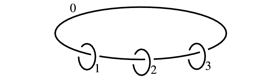
By applying the inverse slam dunk operation (cf. [11, Figure 5.30]), the diagram of Figure 9 can be easily transformed into a star-shaped plumbing as it is given by Figure 10.
The plumbing coefficients on the leg (satisfying and ) are specified by the continued fraction coefficients of the rational number (cf. Equation (2.1)). Notice that all plumbing graphs in the Introduction (Figures 1–7) give rise to –manifolds with small Seifert fibered –manifold boundary.
In a remarkable series of papers [20, 21] Ozsváth and Szabó introduced an invariant for spinc –manifolds: the (mod 2) Ozsváth–Szabó homology group of a closed spinc –manifold is a finite dimensional vector space over the field of two elements. For a rational homology sphere the dimension of this vector space is odd for every spinc structure. We say that a rational homology sphere is an –space if for every spinc structure , that is, has the simplest possible Ozsváth–Szabó homologies.
Recall that a contact structure on any –manifold naturally induces a spinc structure, which we will denote by . In addition, also gives rise to an element , the contact invariant of . (For the definition and basic properties of see [23, 14].)
As the next result (a compilation of theorems of Wu, Ghiggini and Plamenevskaya) shows, tight contact structures on small Seifert fibered –manifolds with simple Ozsváth–Szabó homologies (and ) admit a simple classification scheme. More precisely
Theorem 3.1.
Suppose that the small Seifert fibered –manifold satisfies and is an –space. Then two tight contact structures on are isotopic if and only if .
Proof.
One direction of the statement is obvious: isotopic contact structures are homotopic as –plane fields, hence induce the same spinc structure. The converse, however, is more subtle, since it states that in these –manifolds the spinc structure (which is a homotopic invariant of the contact structure) determines the tight contact structure up to isotopy.
Let denote the star-shaped plumbing graph we get from the surgery diagram of by inverse slam dunks. The corresponding –manifold is then given by a sequence of –handle attachments along the unknots corresponding to the vertices of . Working with a projection now it is easy to see that each unknot can be isotoped until it becomes the Legendrian unknot, i.e., a Legendrian knot isotopic to the unknot with Thurston–Bennequin invariant . The assumption ensures that by adding sufficiently many zig-zags to these Legendrian unknots we end up with a Legendrian link on which contact –surgery results , together with a Stein structure on it [1, 10]. Notice, however, that there is a certain freedom in adding the zig-zags to the unknots: moving a zig-zag from left to right (or from right to left) will change the rotation number of the particular knot, which in turn will change the first Chern class of the resulting Stein structure on . According to a result of Lisca and Matić [13] Stein structures on a fixed –manifold with different first Chern classes induce nonisotopic tight contact structures on the boundary of the –manifold. The number of tight contact structures one can distinguish in this way can be easily computed from the framing coefficients of the graph . Furthermore, it was shown by Plamenevskaya [24] that if two Stein structures on a –manifold induce two contact structures , and for the two Stein structures we have then for the (mod 2 reduced) contact Ozsváth–Szabó invariants we have . In summary, the Legendrian surgery construction described above allowed us to construct a finite set of Stein fillable (hence tight) contact structures on (corresponding to the different choices of left and right zig-zags), and all these structures have different (and nonzero) contact Ozsváth–Szabó invariants.
Now we are ready to prove the theorem. Using convex surface techniques, it was shown by Wu [34] that for a small Seifert –manifold with the above set of Stein fillable contact structures, in fact, contains all tight contact structures on the –manifold at hand. (For these –manifolds the –space condition is automatically satisfied, cf. Lemma 4.1.) For the remaining case we argue as follows: According to [15] the assumption for being an –space implies that admits no transverse contact structure. In [7] this property is translated to a numerical condition for , which in turn, implies that the number of tight contact structures on is bounded above by the number of Stein fillable contact structures constructed by Legendrian surgery along the Legendrian links described above. In short, under the assumption of the theorem, the Legendrian surgery construction described at the beginning of the proof produces all tight contact structures on .
Appealing to the –space property again, now we can easily conclude the proof: if , are nonisotopic tight contact structures on then according to the above said we have . Assuming that for the induced spinc structures holds we easily reach a contradiction: in this case the contact invariants are distinct, nonzero elements, which is clearly impossible. ∎
Remark 3.2.
In fact, a very similar proof (together with the classification of tight contact structures on small Seifert fibered –manifolds with [8]) applies for as well. (It is worth mentioning that if then , therefore any with is still an –space.) The only difference is in the construction of the appropriate –manifold (carrying the Stein structures): for we need to introduce an appropriate Stein –handle as well, cf. the argument of [8]. We will not use this fact in the present paper. A similar statement (that is, that tight contact structures with isomorphic spinc structures are isotopic) is expected in the case when and the –manifold is an –space; for related discussion and partial results see [9]. Most probably the same statement also holds for strongly fillable contact structures on boundaries of negative definite plumbings which are –spaces. Considering all tight contact structures, such a statement cannot be true, since many of these –manifolds are toroidal, hence contain infinite families of homotopic, nonisomorphic tight contact structures. (These infinite families are constructed by inserting Giroux torsions, resulting in contact structures which are not strongly fillable [6].) For strongly fillable structures, however, one can expect that the strong filling can be chosen to be diffeomorphic to the plumbing –manifold, and then the adaptation of the proof above would provide the same result.
4 The proof of Theorem 1.2
We start this section by proving that the result of Theorem 3.1 applies for the plumbing manifolds given by graphs in .
Lemma 4.1.
Suppose that . Then the star-shaped graph is negative definite and the –manifold is an –space.
Proof.
The plumbing graph is negative definite since it embeds in a negative definite lattice [29]. (Alternatively, a simple computation and the application of [18, Theorem 5.2] shows the same.) There are many ways to verify that is an –space. The direct application of the algorithm of [22] (which applies for negative definite plumbing graphs with at most one “bad” vertex) implies the result at once, although this proof involves some computations. (In fact, for graphs in the result is stated in [22], since these graphs involve no “bad” vertices.) Alternatively, we can argue as follows: as [29, Examples 8.3 and 8.4] show, the normal surface singularity defined by admits a rational homology disk smoothing and this property implies that the surface singularity is rational, cf. [29, Proposition 2.3]. (In yet another way, Laufer’s algorithm can be easily applied to verify rationality of the surface singularities defined by graphs in .) The computation presented in [17] shows that the link of a rational singularity is an –space, concluding our argument. ∎
After all these preparations, now we are ready to turn to the proof of Theorem 1.2:
Proof of Theorem 1.2.
Suppose that are symplectic spheres in the symplectic –manifold , intersecting each other –orthogonally, and according to the plumbing tree . By Theorem 2.1 there is a neighbourhood of such that its complement is a strong concave filling of its contact boundary. The contact structure on the boundary induces the spinc structure which extends to as with the property that satisfies the adjunction equality for all (since are all smooth symplectic submanifolds).
Now consider the normal surface singularity given by . As such, it defines a contact structure on its link, which induces the spinc structure . Resolving the singularity doesn’t change this contact structure (and hence the spinc structure ), but provides a –manifold diffeomorphic to , with a spinc structure . Since the vertices of in the resolution correspond to complex curves, the first Chern class of also satisfies the adjunction equality. This shows that , and since is a simply connected –manifold, we conclude that . This fact, however, identifies the spinc structures of the contact structures on , which in the light of Theorem 3.1 implies that the contact structure on induced by the Liouville vector field is isotopic to the one induced on the link of the singularity. This last observation verifies the existence of the desired gluing contactomorphism, hence the symplectic gluing can be performed as in [3], concluding the proof. ∎
References
- [1] Y. Eliashberg, Topological characterization of Stein manifolds of dimension , Int. J. of Math. 1 (1990), 29–46
- [2] Y. Eliashberg, On symplectic manifolds with some contact properties J. Differential Geom. 33 (1991), 233–238.
- [3] J. Etnyre Symplectic convexity in low-dimensional topology, Symplectic, contact and low-dimensional topology (Athens, GA, 1996). Topology Appl. 88 (1998), 3–25.
- [4] R. Fintushel and R. Stern, Rational blowdowns of smooth –manifolds, J. Diff. Geom. 46 (1997), 181–235.
- [5] R. Fintushel and R. Stern, Double node neighborhoods and families of simply connected –manifolds with , J. Amer. Math. Soc. 19 (2006), 171–180.
- [6] D. Gay, Four–dimensional symplectic cobordisms containing three–handles, Geom. Topol. 10 (2006), 1749–1760.
- [7] P. Ghiggini, On tight contact structures with negative maximal twisting on small Seifert manifolds, in preparation 2007.
- [8] P. Ghiggini, P. Lisca and A. Stipsicz, Classification of tight contact structures on small Seifert 3-manifolds with , Proc. Amer. Math. Soc. 134 (2006) 909–916.
- [9] P. Ghiggini, P. Lisca and A. Stipsicz, Tight contact structures on some small Seifert fibered –manifolds, Amer. J. Math., to appear.
- [10] R. Gompf, Handlebody construction of Stein surfaces, Ann. of Math. 148 (1998), 619–693.
- [11] R. Gompf and A. Stipsicz, –manifolds and Kirby calculus, Graduate Studies in Mathematics, 20, AMS 1999.
- [12] H, Grauert, Über modifikationen und exzepotionelle analytische Mengen, Math. Ann. 146 (1962), 331–368.
- [13] P. Lisca and G. Matić, Tight contact structures and Seiberg-Witten invariants, Invent. Math. 129 (1997) 509–525.
- [14] P. Lisca and A. Stipsicz, Ozsváth–Szabó invariants and tight contact –manifolds, I., Geom. Topol. 8 (2004), 925–945.
- [15] P. Lisca and A. Stipsicz, Ozsváth–Szabó invariants and tight contact –manifolds, III., arXiv:math.SG/0505493
- [16] M. Michalogiorgaki, Rational blow–down along Wahl type plumbing trees of spheres and exotic smooth structures on , , arXiv:math.GT/0607608.
- [17] A. Némethi, On the Ozsváth-Szabó invariant of negative definite plumbed 3-manifolds, Geom. Topol. 9 (2005), 991–1042.
- [18] W. Neumann and F. Raymond, Seifert manifolds, plumbing, –invariant and orientation reversing maps, Algebraic and geometric topology (Proc. Sympos., Univ. California, Santa Barbara, Calif., 1977), pp. 163–196, Lecture Notes in Math. 664, Springer, Berlin, 1978.
- [19] H. Ohta and K. Ono, Simple singularities and topology of symplectically filling -manifold, Comment. Math. Helv. 74 (1999), 575–590.
- [20] P. Ozsváth and Z. Szabó, Holomorphic disks and topological invariants for closed three–manifolds, Ann. of Math. 159 (2004), 1027–1158.
- [21] P. Ozsváth and Z. Szabó, Holomorphic disks and three–manifold invariants:properties and applications, Ann. of Math. 159 (2004), 1159–1245.
- [22] P. Ozsváth and Z. Szabó, On the Floer homology of plumbed three–manifolds, Geom. Topol. 7 (2003) 185–224.
- [23] P. Ozsváth and Z. Szabó, Heegaard Floer homologies and contact structures, Duke Math. J. 129 (2005), 39–61.
- [24] O. Plamenevskaya, Contact structures with distinct Heegaard Floer invariants, Math. Res. Lett. 11 (2004), 547–561.
- [25] J. Park, Seiberg–Witten invariants of generalized rational blow–downs, Bull. Austral. Math. Soc. 56 (1997), 363–384.
- [26] J. Park, Simply connected symplectic –manifolds with and , Invent. Math. 159 (2005), 657–667.
- [27] J. Park, A. Stipsicz and Z. Szabó, Exotic smooth structures on , Math. Res. Lett. 12 (2005), 701–712.
- [28] A. Stipsicz and Z. Szabó, An exotic smooth structure on , Geom. Topol. 9 (2005), 813–832.
- [29] A. Stipsicz, Z. Szabó and J. Wahl, Rational blow–downs and smoothings of surface singularities, arXiv:math.SG/0611157.
- [30] M. Symington, Symplectic rational blowdowns, J. Diff. Geom. 50 (1998), 505–518.
- [31] M. Symington, Generalized symplectic rational blowdowns, Algebr. Geom. Topol. 1 (2001), 503–518.
- [32] M. Symington, Four dimensions from two in symplectic topology, in Topology and geometry of manifolds (Athens, GA, 2001), 153–208, Proc. Sympos. Pure Math., 71, Amer. Math. Soc., Providence, RI, 2003.
- [33] A. Weinstein, Contact surgery and symplectic handlebodies, Hokkaido Math. J. 20 (1991), no. 2, 241–251.
- [34] H. Wu, Legendrian vertical circles in small Seifert spaces, Commun. Contemp. Math. 8 (2006), 219–246.