Comultiplicativity of the Ozsváth-Szabó contact invariant

In 2002, Ozsváth and Szabó discovered an invariant of contact 3-manifolds constructed as follows [11]. Given a contact 3-manifold $(Y,\xi)$, we can find a compatible (in the sense of Giroux [5]) open book decomposition $(S,g)$ of $Y$ with connected binding $K\subset Y$. If the genus of $S$ is $k$ then the knot Floer homology, $\widehat{HFK}(-Y,K,-k)\cong\mathbb{Z}$. Moreover, it is possible to find a Heegaard diagram for which the knot Floer homology in this $-k$ th filtration level is generated by an element of the chain complex $\widehat{CFK}(-Y,K)$ which also represents a cycle in the chain complex $\widehat{CF}(-Y)$. The contact invariant $c(\xi)$ is defined to be the image of this cycle in $\widehat{HF}(-Y)$.

The class $c(\xi)$ is well-defined up to sign (we use $\mathbb{Z}_{2}$ coefficients throughout to avoid ambiguity in sign), and it is an invariant of $\xi$ up to isotopy of the contact structure. This invariant encodes information related to the tightness of $\xi$. For instance, Ozsváth and Szabó prove that if $\xi$ is overtwisted, then $c(\xi)=0$. On the other hand, if $\xi$ is Stein fillable or strongly fillable, then $c(\xi)\neq 0$ [11], [10]. In a previous paper we show, in the case of contact structures compatible with genus one, one boundary component open books, that $c(\xi)=0$ if and only if $\xi$ is overtwisted for all but a small family of open books with reducible monodromies [1]. Honda, Kazez, and Matić have since shown this to be the case for all such open books [7], [6], [8]. However, the precise relationship between $c(\xi)$ and the tightness of $\xi$ is still unknown – there are tight contact structures with vanishing contact invariant [4]. In fact, Lisca and Stipsicz conjecture that the contact invariant vanishes for contact structures with positive Giroux torsion [9].

As the contact invariant is defined in terms of a compatible open book decomposition, we often denote $c(\xi)$ by $c(S,g)$. This class satisfies the following naturality property [11]:

In general, it is an open question as to whether tightness of the contact structures compatible with open books $(S,g)$ and $(S,h)$ implies tightness of the contact structure compatible with $(S,hg)$. This question is open even when $h$ is a right-handed Dehn twist $t_{\gamma}$ around a curve $\gamma\subset S$ [3]. Along these lines, however, Theorem 1.1 implies that if $c(S,g)\neq 0$, then $c(S,t_{\gamma}\circ g)\neq 0$. This behavior is generalized in Theorem 1.2, which follows from our main result.

This theorem has the immediate corollary:

The key to this theorem is the observation that the contact invariant satisfies the naturality property below. For any $g$ and $h$ we exhibit a cobordism $X_{g,h}$ with

$$\partial X_{g,h}=-Y_{g}-Y_{h}+Y_{hg}$$

where $Y_{\phi}$ is the three-manifold with open book decomposition $(S,\phi)$. This cobordism induces a chain map (multiplication)

$$m:\widehat{CF}(Y_{g})\otimes_{\mathbb{Z}_{2}}\widehat{CF}(Y_{h})\rightarrow\widehat{CF}(Y_{hg}).$$

If we apply the $\mathrm{Hom}_{\mathbb{Z}_{2}}(-,\mathbb{Z}_{2})$ functor to this expression, we obtain a chain map (comultiplication)

$$\mu:\widehat{CF}(-Y_{hg})\rightarrow\widehat{CF}(-Y_{g})\otimes_{\mathbb{Z}_{2}}\widehat{CF}(-Y_{h}).$$

We show that the contact invariants are natural under the corresponding map

$$\tilde{\mu}:\widehat{HF}(-Y_{hg})\rightarrow\widehat{HF}(-Y_{g})\otimes_{\mathbb{Z}_{2}}\widehat{HF}(-Y_{h})$$

induced on homology. That is

Hence, if $c(S,hg)=0$ then either $c(S,g)=0$ or $c(S,h)=0$, and Theorem 1.2 follows immediately.

In Section 4, we generalize the result of Theorem 1.4 by examining analogous maps on $HF^{+}$. We use this generalization to prove the following theorem.

In Theorem 1.5, $c^{+}(S,\phi)$ denotes the image in $HF^{+}(-Y_{\phi})$ of $c(S,\phi)$ under the natural map $\widehat{HF}(-Y_{\phi})\rightarrow HF^{+}(-Y_{\phi})$. Furthermore, if $(S,g)$ and $(S,h)$ are open books compatible with contact structures $(Y_{g},\xi_{g})$ and $(Y_{h},\xi_{h})$, respectively, then $(S\#_{b}S,g\#h)$ is an open book compatible with the contact structure $(Y_{g}\#Y_{h},\xi_{g}\#\xi_{h}),$ where $\#_{b}$ denotes boundary connected sum.

The following corollaries of Theorem 1.5 provide obstructions to a contact three-manifold with open book $(S,hg)$ having a compatible open book with planar pages. At the same time, we obtain obstructions to the three-manifold $Y_{hg}$ being an $L$-space. The reader should compare these corollaries with those found by Ozsváth, Szabó, and Stipsicz in [13]. In what follows, $\mathfrak{s}(S,\phi)$ denotes the $spin^{c}$ structure associated to the contact 2-plane field which is compatible with $(S,\phi)$.

Honda, Kazez, and Matić give another interpretation of the Ozsváth-Szabó contact class in [7]. We use their reformulation in our proof of Theorem 1.2. Recall that the open book $(S,g)$ is a decomposition of the 3-manifold $Y=S\times[0,1]/\sim$, where $\sim$ is the relation defined by

	$\displaystyle(x,1)\sim(g(x),0),$		$\displaystyle x\in S$
	$\displaystyle(x,t)\sim(x,s),$		$\displaystyle x\in\partial S,\ t,s\in[0,1]$

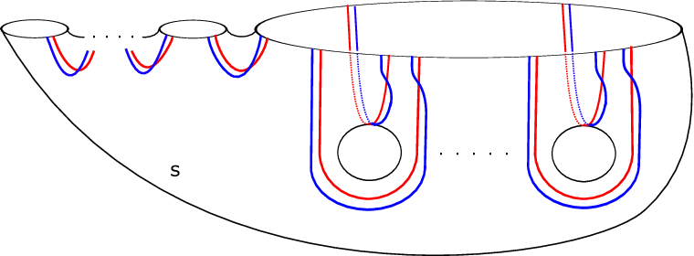
$Y$ has a Heegaard splitting $Y=H_{1}\cup H_{2}$, where $H_{1}$ is the handlebody $S\times[0,1/2]$ and $H_{2}$ is the handlebody $S\times[1/2,1]$. Let $S_{t}$ denote the page $S\times\{t\}$. If $S$ has $n$ boundary components and genus $k$ then the Heegaard surface in this splitting is the genus $2k+n-1$ surface $\Sigma=S_{1/2}\cup-S_{0}$. To specify a pointed Heegaard diagram for $Y$ it remains to describe the $\alpha$ and $\beta$ curves on $\Sigma$ and the placement of a basepoint $z$. Choose $2k+n-1$ disjoint properly embedded arcs $a_{1},\dots,a_{2k+n-1}$ on $\Sigma$ so that $\Sigma\setminus\cup a_{i}$ is topologically a disk. For each $i$ we obtain $b_{i}$ by changing the arcs $a_{i}$ via a small isotopy which moves the endpoints of the $a_{i}$ along $\partial S$ in the direction given by the orientation of $\partial S$ so that $a_{i}$ intersects $b_{i}$ transversely in one point and with positive sign (where $b_{i}$ inherits its orientation from $a_{i}$). See Figure 1 for an illustration of the $a_{i}$ and $b_{i}$ arcs on a surface $S$.

Now define

$$\alpha_{i}=a_{i}\times\{1/2\}\cup a_{i}\times\{0\}$$

$$\beta_{i}=b_{i}\times\{1/2\}\cup g(b_{i})\times\{0\}.$$

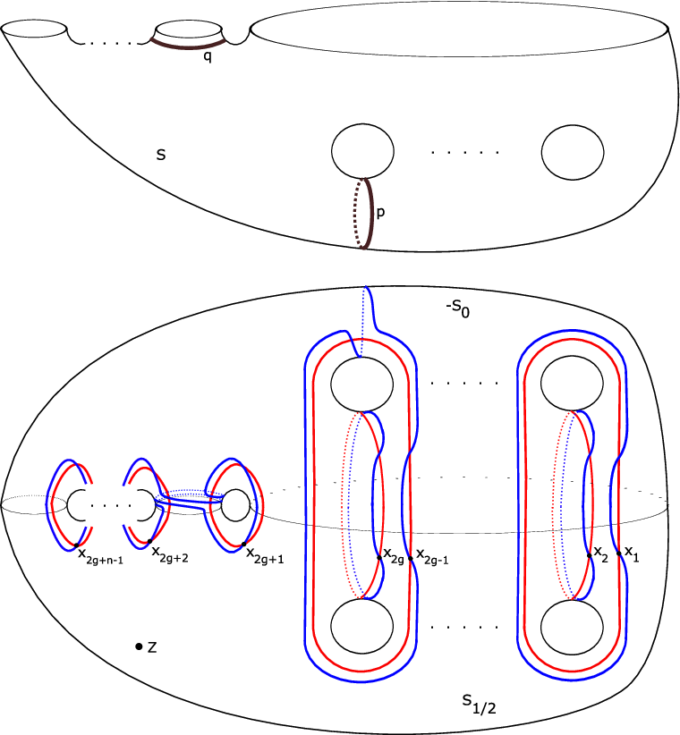
Place the basepoint $z$ in the big region on $S_{1/2}$ (that is, not in one of the thin strip regions). For each $i=1,\dots,2k+n-1$ let $x_{i}$ be the intersection point on $S_{1/2}$ between $\alpha_{i}$ and $\beta_{i}$. Then $\overline{x_{g}}=\{x_{1},\dots,x_{2k+n-1}\}$ is an intersection point between $\mathbb{T}_{\alpha}$ and $\mathbb{T}_{\beta}$ in $Sym^{2k+n-1}(\Sigma)$. Moreover, $\overline{x_{g}}$ is a cycle in $Hom(\widehat{CF}(Y),\mathbb{Z}_{2})=\widehat{CF}(-Y)$ because of the placement of $z$. See Figure 2 for an illustration of the pointed Heegaard diagram for an open book.

Given a surface $S$ with genus $k$ and $n$ boundary components, let $a_{i}$ and $b_{i}$ be the set of properly embedded arcs described above. We construct another set of disjoint properly embedded arcs $c_{i}$ from the $b_{i}$ by changing the arcs $b_{i}$ via a small isotopy which moves the endpoints of the $b_{i}$ along $\partial S$ in the direction given by the orientation of $\partial S$. We require that both $a_{i}$ and $b_{i}$ intersect $c_{i}$ transversely in one point and with positive sign (where $c_{i}$ inherits its orientation from $b_{i}$). For any two diffeomorphisms $g$ and $h$, we construct three sets of attaching curves on the Heegaard surface $\Sigma=S_{1/2}\cup-S_{0}$:

$$\alpha_{i}=a_{i}\times\{1/2\}\cup a_{i}\times\{0\}$$

$$\beta_{i}=b_{i}\times\{1/2\}\cup g(b_{i})\times\{0\}$$

$$\gamma_{i}=c_{i}\times\{1/2\}\cup h(g(c_{i}))\times\{0\}.$$

Once again, we place the basepoint $z$ in the big region of $S_{1/2}$ (outside of the thin strip regions). Then $(\Sigma,\bar{\alpha},\bar{\beta},\bar{\gamma},z)$ is a pointed Heegaard triple-diagram and can be used as in [10] to construct a cobordism $X_{\alpha,\beta,\gamma}$ with

$$\partial X_{\alpha,\beta,\gamma}=-Y_{\alpha,\beta}-Y_{\beta,\gamma}+Y_{\alpha,\gamma}$$

where $Y_{\alpha,\beta}$ is the three manifold with Heegaard decomposition $(\Sigma,\bar{\alpha},\bar{\beta})$ (and similarly for $Y_{\beta,\gamma}$ and $Y_{\alpha,\gamma}$). Such a cobordism induces a chain map

$$\widehat{CF}(Y_{\alpha,\beta})\otimes_{\mathbb{Z}_{2}}\widehat{CF}(Y_{\beta,\gamma})\rightarrow\widehat{CF}(Y_{\alpha,\gamma}).$$

By the description of the Heegaard diagram associated to an open book in section 2, it is clear that

$$Y_{\alpha,\beta}=Y_{g}$$

$$Y_{\beta,\gamma}=Y_{h}$$

$$Y_{\alpha,\gamma}=Y_{hg}.$$

Thus, we have a chain map

(1)

$\displaystyle m:\widehat{CF}(Y_{g})\otimes_{\mathbb{Z}_{2}}\widehat{CF}(Y_{h})\rightarrow\widehat{CF}(Y_{hg}).$

If the pointed Heegaard triple-diagram $(\Sigma,\bar{\alpha},\bar{\beta},\bar{\gamma},z)$ is weakly-admissible then this map is defined on the generators of $\widehat{CF}(Y_{g})\otimes_{\mathbb{Z}_{2}}\widehat{CF}(Y_{h})$ by

$$m(\bar{a}\otimes\bar{b})=\sum_{\bar{x}\in\mathbb{T}_{\alpha}\cap\mathbb{T}_{\gamma}}\sum_{\{\phi\in\pi_{2}(\bar{a},\bar{b},\bar{x})\ |\ \mu(\phi)=0,\ n_{z}(\phi)=0\}}(\#\mathcal{M}(\phi))\bar{x}.$$

In this sum, $\pi_{2}(\bar{a},\bar{b},\bar{x})$ is the set of homotopy classes of Whitney triangles connecting $\bar{a}$, $\bar{b}$, and $\bar{x}$; $\mu(\phi)$ is the expected dimension of holomorphic representatives of $\phi$; $n_{z}(\phi)$ is the algebraic intersection number of $\phi$ with the subvariety $\{z\}\times Sym^{2k+n-2}(\Sigma)\subset Sym^{2k+n-1}(\Sigma)$; and $\mathcal{M}(\phi)$ is the moduli space of holomorphic representatives of $\phi$. For more details, see [10].

As alluded to in the introduction, we apply the $\mathrm{Hom}_{\mathbb{Z}_{2}}(-,\mathbb{Z}_{2})$ functor to the expression in equation 1. If we represent each chain complex diagrammatically by drawing an arrow from $x$ to $y$ whenever $y$ is a term in $\partial x$ or when $y$ is a term in the image of $x$ under the map $m,$ then applying the $\mathrm{Hom}_{\mathbb{Z}_{2}}(-,\mathbb{Z}_{2})$ functor corresponds to reversing the direction of every arrow. Doing so, we obtain a chain map

$\displaystyle\mu:\widehat{CF}(-Y_{hg})\rightarrow\widehat{CF}(-Y_{g})\otimes_{\mathbb{Z}_{2}}\widehat{CF}(-Y_{h}).$

An element in $\widehat{CF}(-Y_{hg})$ is a sum of intersection points $\bar{x}\in\mathbb{T}_{\alpha}\cap\mathbb{T}_{\gamma}$. On such an intersection point the chain map $\mu$ is defined by

$$\mu(\bar{x})=\sum_{\bar{a}\in\mathbb{T}_{\alpha}\cap\mathbb{T}_{\beta},\ \bar{b}\in\mathbb{T}_{\beta}\cap\mathbb{T}_{\gamma}}\sum_{\{\phi\in\pi_{2}(\bar{a},\bar{b},\bar{x})\ |\ \mu(\phi)=0,\ n_{z}(\phi)=0\}}(\#\mathcal{M}(\phi))(\bar{a}\otimes\bar{b})$$

as long as the pointed Heegaard triple-diagram $(\Sigma,\bar{\alpha},\bar{\beta},\bar{\gamma},z)$ is weakly-admissible. To prove Theorem 1.4, we show that

$$\mu(\overline{x_{hg}})=\overline{x_{g}}\otimes\overline{x_{h}}.$$

We complete the proof in two steps. First we show that $(\Sigma,\bar{\alpha},\bar{\beta},\bar{\gamma},z)$ is weakly-admissible. Then we show that there is only one pair $\{\bar{a}\in\mathbb{T}_{\alpha,\beta},\ \bar{b}\in\mathbb{T}_{\beta,\gamma}\}$ for which there exists a homotopy class $\phi\in\pi_{2}(\bar{a},\bar{b},\overline{x_{hg}})$ with $n_{z}(\phi)=0$ and such that $\phi$ has a holomorphic representative. Moreover, $\bar{a}=\overline{x_{g}}$, $\bar{b}=\overline{x_{h}}$, and the number of holomorphic representatives of $\phi$ is one.

References

• [1] J. A. Baldwin. Tight contact structures and genus one fibered knots. 2006, math.SG/0604580.
• [2] J. B. Etnyre. Planar open book decompositions and contact structures. 2004, math.SG/0404267.
• [3] J. B. Etnyre. Lectures on open book decompositions and contact structures. 2005, math.SG/0409402.
• [4] P. Ghiggini. Ozsváth and Z. Szabó invariants and fillability of contact structures. 2005, math.GT/0403367.
• [5] E. Giroux. Convexité en topologie de contact. Comment. Math. Helv., 66:637–677, 1991.
• [6] K. Honda, W. Kazez, and G. Matić. Right-veering diffeomorphisms of a compact surface with boundary I. 2005, math.GT/0510639.
• [7] K. Honda, W. Kazez, and G. Matić. On the contact class in Heegaard Floer homology. 2006, math.GT/0609734.
• [8] K. Honda, W. Kazez, and G. Matić. Right-veering diffeomorphisms of a compact surface with boundary II. 2006, math.GT/0603626.
• [9] P. Lisca and A. Stipsicz. Contact Ozsváth-Szabó invariants and Giroux torsion. 2006, math.SG/0604268.
• [10] P. Ozsváth and Z. Szabó. Holomorphic disks and topological invariants for closed three-manifolds. 2001, math.SG/0101206.
• [11] P. Ozsváth and Z. Szabó. Heegaard Floer homologies and contact structures. 2002, math.SG/0210127.
• [12] P. Ozsváth and Z. Szabó. Holomorphic disks and three-manifold invariants: properties and applications. 2003, math.SG/0105202.
• [13] P. Ozsváth, Z. Szabó, and A. I. Stipsicz. Planar open books and Floer homology. 2005, math.SG/0504403.