A closed formula for the number of convex permutominoes
Abstract
In this paper we determine a closed formula for the number of convex permutominoes of size . We reach this goal by providing a recursive generation of all convex permutominoes of size from the objects of size , according to the ECO method, and then translating this construction into a system of functional equations satisfied by the generating function of convex permutominoes. As a consequence we easily obtain also the enumeration of some classes of convex polyominoes, including stack and directed convex permutominoes.
1 Basic definitions and contents of the paper
A polyomino is a finite union of elementary cells of the lattice , whose interior is connected (see Figure 1 ). Polyominoes are defined up to translations. A polyomino is said to be column convex (resp. row convex) if every its column (resp. row) is connected (see Figure 1 ). A polyomino is said to be convex, if it is both row and column convex (see Figure 1 ).
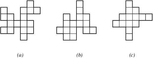
The number of convex polyominoes with semi-perimeter was determined by Delest and Viennot, in [13]:
| (1) |
sequence in [18], the first few terms being:
In the last two decades convex polyominoes, and several combinatorial objects obtained as a generalizations of this class, have been studied by various points of view. For the main results concerning the enumeration and other combinatorial properties of convex polyominoes we refer to [6, 7, 8, 10].
1.1 Permutominoes
Let be a polyomino without holes, having rows and columns, ; we assume without loss of generality that the south-west corner of its minimal bounding rectangle is placed in . Let be the set of its vertices ordered in a clockwise sense starting from the leftmost vertex having minimal ordinate.
We say that is a permutomino if the sets and represent two permutation matrices of . Obviously, if is a permutomino, then , and is called the size of the permutomino.

The two permutations associated with and are indicated by and , respectively (see Figure 2). While it is clear that any permutomino of size uniquely individuates two point-by-point distinct permutations and of , not all the couples of permutations and of such that , define a permutomino, as it was partially investigated in [15] (see Figure 3).

Permutominoes were introduced by F. Incitti in [17] while studying the problem of determining the -polynomials (related with the Kazhdan-Lusztig R-polynomials) associated with a pair of permutations. Concerning the class of polyominoes without holes, our definition (though different) turns out to be equivalent to Incitti’s one, which is more general but uses some algebraic notions not necessary in this paper.
In this paper we deal with the enumeration of convex polyominoes which are also permutominoes, the so called convex permutominoes. From the definition we have that in any convex permutomino , for each abscissa (ordinate) there is exactly one vertical (horizontal) side in the boundary of with that coordinate. It is simple to observe that the previous property is also a sufficient condition for a convex polyomino to be a permutomino.
In [15], using bijective techniques, it was proved that the number of parallelogram permutominoes of size is equal to the th Catalan number,
and moreover, that the number of directed-convex permutominoes of size is equal to half the th binomial coefficient,
The first attempt to count convex permutominoes was made in [5], where the authors considered the couples of permutations which define convex permutominoes, and then obtained an expression for the number of convex permutominoes of size :
but then were not able to derive the generating function, nor the closed form for the number .
In this paper we deal with the same enumeration problem using a different and more immediate approach: we determine a direct recursive construction for the convex permutominoes of a given size, based on the application of the ECO method, which easily leads to the generating function, and finally prove that the number of convex permutominoes of size is:
| (2) |
1.2 ECO method
In this section we will recall some basics about the ECO method, where ECO stands for Enumeration of Combinatorial Objects. Such a method, introduced by Pinzani and his collaborators in [3], is a constructive method to produce all the objects of a given class, according to the growth of a certain parameter (the size) of the objects. Basically, the idea is to perform “local expansions” on each object of size , thus constructing a set of objects of the successive size (see [3] for more details).
The application of the ECO method often leads to an easy solution for problems that are commonly believed “hard” to solve. For example, in [14] the authors give an ECO construction for the classes of convex polyominoes and column-convex polyominoes according to the semi-perimeter. A simple algebraic computation leads then to the determination of generating functions for the two classes.
In [1] it is also shown that an ECO construction easily leads to an efficient algorithm for the exhaustive generation of the examined class. Moreover, an ECO construction can often produce interesting combinatorial information about the class of objects studied, as shown in [3] using analytic methods, or in [4], using bijective techniques. In [2], Banderier et al. reintroduced the kernel method in order to determine the generating function of various types of ECO systems.
Going deeper into formalism, let be a parameter , such that is finite. An operator on the class is a function from to , where is the power set of .
Proposition 1
Let be an operator on . If satisfies the following conditions:
- 1.
-
for each , there exists such that ,
- 2.
-
for each such that , then ,
then the family of sets is a partition of .
This method was successfully applied to the enumeration of various classes of walks, permutations, and polyominoes. We refer to [3], and [16] for further details and results.
The recursive construction determined by can be suitably described through a generating tree, i.e. a rooted tree whose vertices are objects of . The objects having the same value of the parameter lie at the same level, and the sons of an object are the objects it produces through .
If the construction determined by the ECO operator is regular enough it is then possible to describe it by means of a succession rule of the form:
where , and , meaning that object at the root of the generating tree has sons, and the objects , produced by an object are such that , . A succession rule defines a sequence of positive integers, where is the number of nodes at level of the generating tree, assuming that the root is at level .
2 Generation of convex permutominoes
Let be the set of convex permutominoes of size . In order to define the ECO construction for convex permutominoes, we need to point out a simple property of their boundary, related to reentrant and salient points. So let us briefly recall the definition of these objects.
Let be a polyomino; starting from the leftmost point having minimal ordinate, and moving in a clockwise sense, the boundary of can be encoded as a word in a four letter alphabet, , where (resp. , , ) represents a north (resp.east, south, west) unit step. Any occurrence of a sequence , , , or in the word encoding defines a salient point of , while any occurrence of a sequence , , , or defines a reentrant point of (see for instance, Figure 4).
In [12] and successively in [9], in a more general context, it was proved that in any polyomino the difference between the number of salient and reentrant points is equal to .

Let us turn to consider the class of convex permutominoes. In a convex permutomino of size the length of the word coding the boundary is , and we have salient points and reentrant points; moreover we observe that a reentrant point cannot lie on the minimal bounding rectangle. This leads to the following remarkable property:
Proposition 2
The set of reentrant points of a convex permutomino of size defines a permutation matrix of , .
For simplicity of notation, and to clarify the definition of the upcoming ECO construction, we agree to group the reentrant points of a convex permutomino in four classes; in practice we choose to represent the reentrant point determined by a sequence (resp. , , ) with the symbol (resp. , , ). Using this notation we can state that each convex permutomino of size can be uniquely represented by the permutation matrix defined by its reentrant points, which has dimension , and uses the symbols .

2.1 The ECO operator
Let ; the number of cells in the rightmost column of is called the degree of . For any we partition the class into three distinct classes. In order to define these classes, let us consider the following conditions on a convex permutomino:
- U1
-
: the uppermost cell of the rightmost column of the polyomino has the maximal ordinate among all the cells of the polyomino;
- U2
-
: the lowest cell of the rightmost column of the polyomino has the minimal ordinate among all the cells of the polyomino.

We say that a convex permutomino belongs to class:
For simplicity sake, each permutomino in class (resp. , ) and degree is represented by the label (resp. , ). For instance, the four permutominoes depicted in Figure 6 have labels , , , , respectively. We assume that the single cell permutomino belongs to class , then it has the label .
Our aim is now to use the property stated in Proposition 2 to define an ECO operator which defines a recursive construction of all the objects of size in a unique way from the objects of size . The operator acts on a convex permutomino performing some local expansions on the cells of its rightmost column. In order to define these operations let us consider a generic permutomino of size , let us indicate by (resp. ) the columns (resp. rows) of numbered from left to right (resp. bottom to top), and by (resp. ) the number of cells in the th column (resp. th row), with . The four operations of will be denoted by , , , and , and below we give a detailed description of each of them:

-
if satisfies condition U1, then adds a new column made of cells on the right of , according to Figure 7.
It is clear that the obtained polyomino is a convex permutomino of size , still satisfying condition U1; the rightmost reentrant point in such new permutomino is of type (this is the reason why we have called the reentrant points with the same name of the operations on permutominoes).
-
it can be performed on each cell of ; so let be the th cell of , from bottom to top, with . Operation adds a new row above the row containing (of the same length), and a new column on the right of , made of cells, as illustrated in Figure 8.
Observe that, since the new added row is long as the row below it, we ensure that the obtained polyomino has a unique horizontal side at level , while adding the new column from bottom to level we ensure that the obtained polyomino has a unique vertical side at abscissa , hence the basic property of permutominoes is preserved.

Figure 8: Operation performed on a cell of the rightmost column of a polyomino in class . The cell is filled in black, the added row and column have been highlighted. Then it is clear that, for any , the obtained polyomino is a convex permutomino of size , and its rightmost reentrant point is of type .
-
it can be performed on each cell of ; so let be the th cell of , from bottom to top, with . Operation adds a new row below the row containing (of the same length), and a new column on the right of , made of cells, as illustrated in Figure 9.

Figure 9: Operation performed on a cell of the rightmost column of a polyomino in class . The cell is filled in black, the added row and column have been highlighted. It is clear that, for any , the obtained polyomino is a convex permutomino of size , and its rightmost reentrant point is of type .
-
if satisfies condition U2, then adds a new column made of cells on the right of , according to Figure 10.
It is clear that the obtained polyomino is a convex permutomino of size , still satisfying condition U2; the rightmost reentrant point in such new permutomino is of type .

Figure 10: Operation performed a polyomino in class .
As we already mentioned, the operations performed by on a convex permutomino depend on the family to which belongs. So let us consider the different cases:
- 1.
belongs to class . The operator performs on operations , and one application of and for any cell in . So, let be the degree of , the application of to produces different convex permutominoes of size (see Figure 11).

Figure 11: The operator applied to a permutomino of class ; the added rows and columns are highlighted, and the applied operation is mentioned below. More formally, applying to a convex permutomino of label , we have different permutominoes, two with label , and two with label . This can be formalized by the production:
- 2.
belongs to class . There are two possibilities:
-
i. satisfies U1 (and not U2). The operator performs on operation , and one application of operations and for any cell in .
-
ii. satisfies U2 (and not U1). The operator performs the following operations: The operator performs on operations , and one application of operations and for any cell in (see Figure 12).

Figure 12: The operator applied to a permutomino of class , satisfying U2 (and not U1); the added rows and columns are highlighted, and the applied operation is mentioned below.
In both cases, being be the degree of , the application of to produces different convex permutominoes of size . More formally, applying to a convex permutomino of label , we have different permutominoes, with labels , and . This can be formalized by the production:
-
- 3.
belongs to class . The operator performs on an application of operations and for any cell in . So, let be the degree of , the application of to produces different convex permutominoes of size . More formally, applying to a convex permutomino of label , we have different permutominoes, two with labels . This can be formalized by the production:
Proposition 3
The operator satisfies conditions 1. and 2. of Proposition 1.
Proof. We have to prove that any convex permutomino of size is uniquely obtained through the application of the operator to a convex permutomino of size . So let , and, as usual, let us indicate by (resp. ) the columns (resp. rows) of numbered from left to right (resp. bottom to top), and by (resp. ) the number of cells in the th column (resp. th row), with . We look at the rightmost reentrant point of , which is unique due to Proposition 2, and we have the following four possibilities:
- 1.
the rightmost reentrant point of is of type , i.e. ; due to the permutomino definition, it is clear that , then has been produced through the application of operation to the permutomino , obtained removing column from (see Figure 7);
- 2.
the rightmost reentrant point of is of type , and then necessarily ; let be the permutomino of obtained by removing the column and the row from . Is is then clear that is produced through the application of operation to the -th cell (from bottom to top) of (see Figure 8);
- 3.
the rightmost reentrant point of is of type , and then necessarily ; let be the permutomino of obtained by removing the column and the row from . Is is then clear that is produced through the application of operation to the -th cell (from bottom to top) of (see Figure 9);
- 4.
the rightmost reentrant point of is of type , also with ; due to the permutomino definition, it is clear that , then has been produced through the application of operation to the permutomino , obtained removing column from (see Figure 10).
The growth of convex permutominoes defined by the ECO operator can be suitably represented in terms of the succession rule :

The root of the tree is , which is the label of the one cell polyomino.
3 Enumeration of convex permutominoes
In this section we will determine the generating function of convex permutominoes according to various parameters, using the simple remark that the number of convex permutominoes of size is given by the number of objects at level of the generating tree of , , assuming without loss of generality that the root of the tree is at level .
Throughout this section, we will use the following notation:
-
- is the set of labels of the generating tree of ;
-
- (resp. , ) is the set of labels (resp. , ), , in the generating tree of .
Moreover, for any convex permutomino , let (briefly, ) be the label of , and (briefly, ) be the size of . Our aim is to determine the generating function:
since in particular is the generating function of convex permutominoes according to the size. To do this we need to consider the following auxiliary generating functions:
- -
-
, i.e. the generating function of ,
- -
-
, i.e. the generating function of ,
- -
-
, i.e. the generating function of .
Clearly, . From the productions of we obtain the following relations concerning :
hence we have that
| (3) |
Then we are able to write down the equation for :
Let ; the previous equation can be re-written as:
| (4) |
Equation (4) has two unknowns: , and . Applying the kernel method (as explained in detail in [2]) we look for the value of for which the factor on the left multiplying is equal to zero, i.e. the solution of the kernel
Of the two solutions we observe that only
is a formal power series with positive coefficients. Substituting in we have:
which leads to:
| (5) |
Replacing the value of into (4) we obtain
| (6) |
Finally, from the productions of we derive the following equation for :
Again, we set ; the previous equation can be re-written as:
| (7) |
As for equation (4), also (7) can be solved using the kernel method. Here the kernel has a unique solution:
replacing with in we have:
which leads to:
| (8) |
Replacing the expression of in (7) we can obtain also . Finally we have the generating function:
| (9) |
and the generating function of convex permutominoes according to the size, which gives, after some simplifications:
| (10) |
Starting from (10) and performing standard calculations we have the following closed form for the number of convex permutominoes of size :
| (11) |
The first terms of the sequence are
We remark that while both the left and the right summands of (11) are in [18] (sequence A079028 and A002457, respectively), the sequence is not present in the Sloane database.
Finally we observe that also the number of stack and directed convex permutominoes can be easily obtained from the previous computation.
In fact a stack permutomino can be uniquely represented by a permutomino in class having the same size. Hence the generating function of stack permutominoes is given by , and then the number of stack permutominoes of size , as already stated in [15], is equal to .
Similarly, a directed convex permutomino can be uniquely represented by a permutomino in class or one in class satisfying U1, having the same size. Hence the generating function of directed convex permutominoes is given by
and then the number of directed convex permutominoes of size , as already stated in [15], is equal to
| (12) |
4 Further work
In this paper we solve the problem of determining a closed formula for the number of convex permutominoes with a fixed size. We reach this goal by defining a recursive construction of all the permutominoes of size starting from those of size , for any .
Several problems on the class of permutominoes however remain still open. Below we propose a small list of the problems which we are interested in, and we would like to tackle in some future work:
- 1.
- 2.
-
we believe that the ECO construction of convex permutominoes can be extended to the class of column-convex permutominoes. One of the problems with this class is that here Proposition 2 does not hold as shown in Figure 14.

Figure 14: A column-convex permutominoes: its reentrant points do not satisfy the statement of Proposition 2. - 3.
-
enumerate convex permutominoes according to the area, i.e. the number of cells of the permutomino. The ECO construction we have determined easily leads to a functional equation satisfied by the generating function of convex permutominoes according to the area and the size of the permutomino; however, then we have not been able to solve this equation.
References
- [1] Bacchelli, S., Barcucci, E., Grazzini, E., Pergola, E.: Exhaustive generation of combinatorial objects by ECO, Acta Informatica 40 (2004) 585-602.
- [2] Banderier, C., Bousquet-Mélou, M., Denise, A., Flajolet, P., Gardy, D., Gouyou-Beauchamps, D.: Generating functions for generating trees, Disc. Math. 246 (2002) 29-55.
- [3] Barcucci, E., Del Lungo, A., Pergola, E., Pinzani, R.: ECO: a methodology for the Enumeration of Combinatorial Objects., J. Diff. Eq. and App. 5 (1999) 435-490.
- [4] Barcucci, E., Frosini, A., Rinaldi, S.: On directed-convex polyominoes in a rectangle, Disc. Math., 298 (2005) 62-78.
- [5] Boldi, P., Lonati, V., Radicioni, R., Santini, M.: The number of convex permutominoes., Rapporto Interno n.311-06, Università degli Studi di Milano, available electronically at http://santini.dsi.unimi.it/ santini/FTP/papers/ridsi-311-06.pdf.
- [6] M. Bousquet-Mèlou, A method for the enumeration of various classes of column-convex polygons, Discrete Math. 154 (1996) 1–25.
- [7] M. Bousquet-Mèlou, A. J. Guttmann, Enumeration of three dimensional convex polygons, Ann. of Comb. 1 (1997) 27–53.
- [8] Brak, R., Guttmann, A. J., Enting, I. G.: Exact solution of the row-convex polygon perimeter generating function, J. Phys. A 23 (1990) L2319–L2326.
- [9] Brlek, S., Labelle, G., Lacasse, A.: A Note on a Result of Daurat and Nivat, Lecture Notes in Computer Science, Springer Berlin/Heidelberg, Vol. 3572 (2005) 189-198.
- [10] Chang, S.J., Lin, K.Y.: Rigorous results for the number of convex polygons on the square and honeycomb lattices, J. Phys. A: Math. Gen. 21 (1988) 2635-2642.
- [11] Conway, J.H., Lagarias, J.C.: Tiling with polyominoes and combinatorial group theory, J. Comb. Th. A 53 (1990) 183-208.
- [12] Daurat, A., Nivat, M.: Salient and reentrant points of discrete sets, Discrete Applied Mathematics 151 (2005) 106-121.
- [13] Delest, M., Viennot, X.G.: Algebraic languages and polyominoes enumeration, Theor. Comp. Sci. 34 (1984) 169-206.
- [14] Del Lungo, A., Duchi, E., Frosini, A., Rinaldi, S.: On the generation and enumeration of some classes of convex polyominoes, Electronic J. Combinatorics, 11 (2004), #R60.
- [15] Fanti, I., Frosini, A., Grazzini, E., Pinzani, R., Rinaldi, S.: Polyominoes determined by permutations, (submitted).
- [16] Ferrari, L., Pergola, E., Pinzani, R., Rinaldi, S.: An algebraic characterization of the set of succession rules, Theor. Comp. Sci., 281 (1-2) (2002) 351-367.
- [17] Incitti, F., Permutation diagrams, fixed points and Kazdhan-Lusztig -polynomials, Ann. Comb., 10, N.3, (2006) 369-387.
- [18] Sloane, N.J.A.; The On-Line Encyclopedia of Integer Sequences, http://www.research.att.com/ njas/sequences/