Direct Matrix Method for Computing Jacobians of Discretized Integro-diff. Eqs. \runauthorK. T. Chu
A Direct Matrix Method for Computing Analytical Jacobians of Discretized Nonlinear Integro-differential Equations
Abstract
In this pedagogical article, we present a simple direct matrix method for analytically computing the Jacobian of nonlinear algebraic equations that arise from the discretization of nonlinear integro-differential equations. The method is based on a formulation of the discretized equations in vector form using only matrix-vector products and component-wise operations. By applying simple matrix-based differentiation rules, the matrix form of the analytical Jacobian can be calculated with little more difficulty than that required when computing derivatives in single-variable calculus. After describing the direct matrix method, we present numerical experiments demonstrating the computational performance of the method, discuss its connection to the Newton-Kantorovich method, and apply it to illustrative 1D and 2D example problems. MATLAB code is provided to demonstrate the low code complexity required by the method.
Keywords: analytical Jacobian; numerical methods; matrix calculus; Newton’s method; integro-differential equations
1 Introduction
Many numerical methods for solving nonlinear integro-differential equations require computation of the Jacobian for the system of algebraic equations that arises when the continuous problem is discretized. For example, any Newton’s method calculation requires computation of the Jacobian (exactly or approximately) during each Newton iteration [28, 29]. Unfortunately, calculation of the Jacobian can be a time-consuming and error-prone procedure for both the computer and the scientific programmer.
In this pedagogical article, we present a simple direct matrix method for calculating analytical Jacobians of discretized, nonlinear integro-differential equations. The direct matrix method produces the Jacobian for the discretized equations directly in matrix form without requiring calculation of individual matrix elements. The essential idea is to first write the discretized, integro-differential equation explicitly in terms of discrete operators (e.g., differentiation and quadrature matrices [8, 22, 41]) and then use simple matrix-based differentiation rules to calculate the Jacobian directly [10, 12, 13, 15]. The key observation underlying this approach is that there is a tremendous amount of structure in the nonlinear algebraic equations that arise from the discretization of nonlinear integro-differential equations. By taking advantage of this structure, the calculation of analytical Jacobians is reduced to nearly the level of complexity required to compute derivatives of scalar, single variable functions.
The operator-based approach of expressing and analyzing discretized differential equations has been used implicitly by the scientific computing community for decades, especially in the context of the Newton-Kantorovich and related methods [6, 7, 30]. However, a direct matrix approach seems to have been first formally described in one place by Chen who presented a collection of rules formulated in terms of specially defined matrix products [10, 12, 13]. In addition to using the method to solve nonlinear partial differential equations [12, 14], Chen used his formulation of the method to develop several interesting theoretical results (e.g., stability analysis of numerical methods for nonlinear time-dependent problems) based on the observation that when a nonlinear differential equation only has polynomial nonlinearities, there is a very close relationship between the discretized nonlinear differential equation and its Jacobian [10, 11].
Mathematically, the present formulation of the direct matrix method is equivalent to Chen’s approach. However, rather than introducing special matrix products, we rely solely on standard linear algebra operations augmented by component-wise operations (e.g., the Hadamard or Schur product [25]). In addition, we have chosen to use MATLAB notation in our formulation because of its prevalence in modern scientific computing. Working in MATLAB notation has the added benefit of making it almost trivial to translate the analytical calculations into working numerical code11 1 With today’s powerful desktop and laptop computers, MATLAB is quite capable of handling moderate-sized production work..
Another feature of our formulation, which is also present to some extent in [10], is the emphasis on the analogy between calculation of Jacobians for discretized, nonlinear integro-differential equations and calculation of derivatives for scalar functions of a single variable. To help strengthen the analogy with single-variable calculus, we organize the operations required to compute a Jacobian as a short list of simple differentiation rules.
This article is organized as follows. In the remainder of this section, we compare the direct matrix method with several common methods for computing Jacobians. In Section 2, we present the direct matrix method, including a discussion of its computational performance and its relation to the Newton-Kantorovich method. Finally, in Section 3, we apply the direct matrix method to two examples (one 1D and one 2D) from the field of electrochemical transport. To demonstrate the low code complexity required by the direct matrix method, MATLAB code for the example problems is provided in the appendices. Throughout our discussion, we will focus solely on collocation methods where the continuous and discrete forms of the integro-differential equation have essentially the same structure. However, it is important to recognize that the direct matrix method can also be used for Galerkin methods by applying it directly to the weak-form of the problem.
1.1 Comparison with Common Methods for Computing Jacobians
One common approach for obtaining the Jacobian of a discretized, nonlinear integro-differential equation is to compute it numerically using finite differences of the grid function or expansion coefficient values [28, 29]. Unfortunately, numerical computation of the Jacobian can be time consuming for some problems. Depending on the numerical method, it might be possible to reduce the computational cost of a numerical Jacobian by taking advantage of the sparsity pattern in the Jacobian [19, 20, 29], but determining the sparsity pattern can be complicated for nontrivial problems.
As an example, consider the Poisson-Nernst-Planck equations for electrochemical transport [4, 17, 36]:
| (1) | |||||
| (2) | |||||
| (3) |
where are cation and anion concentrations, respectively, and is the electric potential, and is a dimensionless physical parameter related to the dielectric constant of the electrolyte. The first two of these are the Nernst-Planck equations for ion transport and are simply conservation laws for cations and anions [33, 36]. The last equation is the Poisson equation [27], which provides closure for the Nernst-Planck equations. Note that in (3), the local charge density has been written in terms of the individual ions, which are the only source of charge density in many electrochemical systems. (1) – (3) form a nonlinear parabolic system of partial differential equations, which suggests that we use an implicit time-stepping scheme to numerically solve the equations. This choice, however, requires that at time , we solve a nonlinear system of equations for which depends on an auxiliary variable which is in turn related to through the Poisson equation. Note that in order to numerically compute the Jacobian for the resulting nonlinear system of equations for , we must solve the Poisson equation for each perturbation to the current iterate of . Therefore, for a pseudospectral discretization of (1) – (3) using grid points, numerically computing the Jacobian requires operations, which is much higher than the elements in the Jacobian22 2 While low-order discretization of the equations do not show this same disparity in the computation time and the number of elements (requiring operations for elements), they typically require many more grid points to produce an accurate solution..
Using an analytical Jacobian is one way to avoid the computational cost associated with numerical Jacobians. In principle, it is straightforward to derive the analytical Jacobian for the system of algebraic equations that arises when a nonlinear integro-differential equation is discretized. Index notation (also known as tensor notation) is perhaps the most common technique used to calculate analytical Jacobians. The basic idea behind the index notation method is to write the discretized form of the differential equation using index notation and then use tensor calculus to compute individual matrix elements in the Jacobian. For example, for a finite-difference or pseudospectral discretization, the discretized equations can be written in the form:
| (4) |
for where and are the value of the solution and the discretized differential equation at the -th grid point (or more generally, the -th collocation point). Boundary conditions are included in this formulation by using the discretized boundary conditions (rather than the integro-differential equation) at grid points on the boundary (or immediately adjacent to if no grid points reside on the boundary)33 3 Care must be exercised when imposing boundary conditions, especially when using pseudospectral methods [23].. The -th element of the Jacobian, , for (4) is simply the partial derivative of with respect to : . While simple and straightforward, index notation suffers from the disadvantage of being somewhat tedious and error-prone. The main challenge in using index notation is keeping track of all of the indices when writing out and computing partial derivatives of the discrete equations.
Automatic differentiation [24, 26] offers an important alternative when exact Jacobians are desired. Because it generates code for computing the Jacobian directly from the code used to evaluate the residual, automatic differentiation completely eliminates the possibility of human error when deriving the exact Jacobian and implementing it in code. Recent developments have made automatic differentiation available in several common programming languages (including MATLAB [37]). While useful, automatic differentiation still takes some effort to use and may not always generate the most compact, efficient code. Active development in this area will certainly continue to improve the usability of automatic differentiation software and the performance of generated code.
The direct matrix method has several advantages over the methods discussed in this section. First, the direct matrix method yields a more accurate Jacobian than finite differences and generally in less time (see Section 2.4). Second, because the method is based on simple differentiation rules, the calculation is straightforward and less prone to error than the index notation approach. The differentiation rules also make it easier to calculate the Jacobian for differential equations which depend on auxiliary variables, such as (1) – (3). From a programming perspective, calculation of the Jacobian directly in matrix form facilitates implementation of numerical methods for nonlinear problems in languages that have built-in support for matrix and vector operations (e.g., MATLAB and Fortran 95). Finally, having the Jacobian available in matrix form can be useful for analyzing properties of numerical methods [10]. While it may be possible to to convert the element-wise representation of the Jacobian derived using index notation for simple problems, this step can be challenging for more complex problems44 4 Interestingly, the conversion from element-wise to matrix representation of the Jacobian often reveals the close relationship between the Jacobian for the discrete equations and the underlying structure of the original integro-differential equation..
2 The Direct Matrix Method
There are two basic ideas underlying the direct matrix method for calculating analytical Jacobians of discretized, integro-differential equations. First, rather than writing the discretized, integro-differential equations at each of the collocation points in terms of individual elements of the solution vector, we write the entire system of equations as a single vector equation expressed explicitly in terms of matrix-vector products and component-wise multiplication (e.g., Hadamard products). Second, the analytical Jacobian for the discretized system of equations is computed directly in matrix form by using simple differentiation rules that are reminiscent of those used to compute derivatives in single-variable calculus. In this section, we develop both of these ideas in detail. Towards the end of the section, we comment on the computational performance of the direct matrix method and its relationship to the Newton-Kantorovich method [8].
2.1 Matrix-vector Representation of Discretized Equations
Writing the discretized, nonlinear integro-differential equation explicitly in terms of basic linear algebra and component-wise algebraic operations is the initial step of the direct matrix method. Because of the similarities in the structure between the discrete and continuous forms of the equations, the procedure is very straightforward. First, convert all differentiation and integration operators into their discrete analogues. Since both of these operations are linear, they become multiplication of vectors representing grid functions by differentiation and quadrature matrices, respectively:
| (5) | |||||
| (6) |
where the hat accent indicates a discretized field variable and and are the differentiation and quadrature matrices associated with the choice of computational grid.
Next, convert all point-wise algebraic operations and function evaluations in the continuous equations to component-wise algebraic operations and function evaluations in the discrete equations. Some examples of the conversion process include:
| (7) | |||||
| (8) | |||||
| (9) | |||||
| (10) |
In these examples, we have adopted the MATLAB convention of using to represent component-wise application of the operation. Also, note that we have abused notation for component-wise function evaluations – represents the vector
| (11) |
not an arbitrary vector function of the entire solution vector . Throughout our discussion, we will indicate component-wise and general functions of by using lowercase and uppercase variables, respectively.
2.1.1 Differential and Integral Operators in Multiple Space Dimensions
It is important to emphasize that the matrix-vector representation is not restricted to scalar field equations or functions of a single variable. Handling vector equations is simple – vector equations may be treated as systems of equations and vector operations may be expressed in component-wise form.
The construction of differential and integral operators for functions of multiple variables is slightly more complicated but straightforward. First, we represent grid functions as a 1D vector by selecting an ordering of the grid points. Then, we derive the differentiation and integration matrices associated with this choice of ordering. While there is no unique mapping from a multi-dimensional grid to a 1D vector, it is important to choose the ordering of the grid points carefully because it directly affects the ease with which differentiation and integration matrices can be derived.
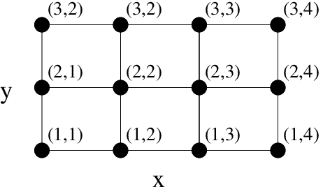
For problems on logically rectangular computational domains, the computational grid may be constructed as a Cartesian product of one-dimensional grids [41]. The result is a structured grid (possibly non-uniform depending on the discretization in each coordinate direction). To represent a grid function as a 1D vector, the most natural way to flatten the grid is by using a lexicographic order for the grid indices. For example, on the small by Cartesian grid in Figure 1, we could order the grid function, , one row at a time:
| (12) |
where is the value of at . With this choice of ordering, discrete partial derivative operators are given as Kronecker product of the differentiation matrices with identity matrices [41]. For the example in Figure 1, the partial differentiation matrices are
| (13) | |||||
| (14) |
where and are the 1d differentiation and identity matrices of size and denotes the Kronecker product. Note that care must be taken to ensure that the order of the Kronecker products is consistent with the ordering of the grid function vector.
To illustrate these ideas, let us consider the discretized forms of the curl and divergence of a vector field, . Once we have chosen an ordering of the grid points and derived the corresponding partial differentiation matrices , , and , the discrete curl operator may be easily written as
where , , and are the components of . The discrete divergence operator is also straightforward to derive:
| (19) |
Boundary Conditions
For problems in multiple space dimensions, it is often convenient to include discretized boundary conditions in a matrix-vector representation by first breaking the full differentiation and integration matrices into multiple components. Each component is defined by the grid points that it contributes to and the grid points it receives contributions from. For instance, it may be convenient to decompose a differentiation matrix into four mutually exclusive components that: (1) use interior points and contribute to interior points, (2) use interior points and contribute to boundary points, (3) use boundary points and contribute to interior points, and (4) use boundary points and contribute to boundary points. Splitting the differentiation and integration matrices into separate components can be helpful when computing residuals and Jacobians for the different types of grid points in the computational domain.
Deriving these components is straightforward using zeroth-order restriction and prolongation matrices [9]. A zeroth-order restriction matrix is a matrix of zeros and ones which extracts a desired subset of elements from a vector. A zeroth-order prolongation matrix is also a matrix of zeros and ones, but it injects the elements of a restricted vector into a desired subset of the elements of a full-length vector. If are the (flattened) indices of a subset of points from grid points, then the associated restriction matrix, , would be an matrix, , with ones at the positions . The associated prolongation matrix, , that injects a vector of length into the positions of a vector of length is simply the transpose of : . For example, the restriction and projection matrices for the two interior points of the grid in Figure 1 are given by
| (20) |
To derive the differentiation matrix that uses values from grid points and contributes to grid points , we use the prolongation matrix for set to expand the restricted grid function associated with into a full-length vector and the restriction matrix for set to compress derivative grid function to the set :
| (21) |
Restricted integration matrices are derived in exactly the same manner.
2.2 Simple Differentiation Rules for Computing Exact Jacobians
Once the continuous equations have been put in a discretized form that is expressed explicitly in terms of matrix-vector products and component-wise operations, the analytical Jacobian for the discretized equations can be calculated by applying a few simple matrix-based differentiation rules. Because the differentiation rules are expressed completely in matrix form without any reference to individual elements in the Jacobian matrix, they allow us to compute the Jacobian directly in matrix form. In this section, we list these differentiation rules, which are essentially results from multivariate and matrix calculus applied specifically to the structure of discretized integro-differential equations.
2.2.1 Matrix-Vector Product Rule
The Jacobian of a matrix-vector product (which corresponds to a linear operator acting on a function in the continuous equations) is just the matrix itself:
| (22) |
For example, the Jacobian of the discretized derivative of , , is just .
2.2.2 Diagonal Rule
The Jacobian of a component-wise function of a grid function is a diagonal matrix with diagonal entries given by :
| (23) |
In essence, the diagonal rule is a way to use matrix notation to represent the fact that the differential in the -th component of only depends on the change in the -th component of and is given by , As an example, the Jacobian of is .
2.2.3 Chain Rules
The Jacobian of a matrix times an arbitrary function, , of all of the components of is times the Jacobian of :
| (24) |
Similarly, the Jacobian of a function, , when its argument is a matrix times the grid function is the Jacobian of evaluated at times :
| (25) |
These rules are simply the chain rules for vector fields from multivariate calculus [1].
2.2.4 Product Rule
To compute the Jacobian of a component-wise product of general functions and of a grid function , we use the product rule:
| (28) |
The derivation of the product rule follows from the expression for the variation of the -th component of
| (29) |
which yields the Jacobian
| (30) |
2.3 Example Jacobian Calculations
As our first example, let us consider the 1D Poisson equation:
| (31) |
To put this in discretized form, we need only replace the continuous second derivative operator by a discrete analogue:
| (32) |
Here, we have chosen to apply the discrete single derivative operator twice. Via a direct application of the matrix-vector product rule (22), the Jacobian of the left-hand side of this equation is easily found to be . Since this is a linear equation, there would not normally be a need to compute the Jacobian of the left hand side of this equation. Moreover, the Jacobian for this example is very easy to calculate using alternative means (or even by inspection). We merely present it to illustrate the direct matrix method on a simple model problem.
As a less trivial, let us calculate the Jacobian for the discretized form of the nonlinear function
| (33) |
Converting this function to discrete form, we obtain
| (34) |
Using the product rule (28), we find that the the Jacobian is given by
| (35) |
Then applying the diagonal rule (23) and the matrix-vector product rule (22), we find that
| (36) |
which can be simplified to
| (37) |
by observing that
As a final example, let us calculate the Jacobian for the nonlinear algebraic equations that arise when solving the one-dimensional version of (1) – (3) using a simple backwards Euler discretization in time. Using the direct matrix approach for the spatial discretization, the nonlinear algebraic equations for and that need to be solved at each time step are:
| (38) | |||||
| (39) | |||||
| (40) |
where are the concentrations at the current time step and is the time step size. It is important to mention that several of the rows in (40) will typically be replaced to impose the discretized form of the boundary conditions for . For illustrative purposes, let us suppose that we have simple Dirichlet boundary conditions for . In this situation, (40) is only imposed at interior grid points [41].
Using the simple differentiation rules from the previous section, the Jacobian of (38) with respect to is
| (41) |
where is the identity matrix and is the Jacobian of with respect to . To eliminate from this expression, we simply apply the differentiation rules to (40) with two rows eliminated for the boundary conditions and solve for the interior portion of :
| (42) |
where is the submatrix of that remains when all of the columns and rows corresponding to boundary grid points have been removed. Since the boundary values of are fixed and the values of at the boundaries do not affect the potential in the interior, the full Jacobian is given by
| (43) |
where we have assumed that the first and last grid points correspond to boundary points. It is important to recognize that the form for in (43) is specific to problems with Dirichlet boundary conditions for . For other boundary conditions, the inversion of the equation for generally leads to different forms for the Jacobian.
The Jacobian for (38) can now be explicitly computed by substituting (43) into (41). The similar expression for the Jacobian of (39) is obtained using an analogous procedure. Using the direct matrix approach, we have reduced the calculation of the Jacobian to (cost of matrix-inversion and matrix-matrix multiplies) compared to the cost for computing a numerical Jacobian for high-order spatial discretizations. It is worth pointing out that in this example, the Jacobian for the concentrations does not depend explicitly on because the Poisson equation is linear. As a result, there is no need to solve for in order to compute the Jacobians for (38) and (39). For general problems, the Jacobian may depend on the auxiliary variable, so it might be necessary to solve the constraint equation. However, because only one solve for the auxiliary variables is required with the direct matrix method, the cost of computing the Jacobian is still dramatically reduced compared to using finite differences.
2.4 Computational Performance
In general, using the direct matrix method to compute a Jacobian is faster than calculating a numerical Jacobian. As mentioned in the previous section, the performance difference is expected to be large when auxiliary variables are involved in the expression of the residual. However, the direct matrix method yields higher performance even for problems where the residual is relatively simple.


Figure 2 compares the performance of the direct matrix method against the MATLAB numjac() function for the two example problems discussed in Section 3. As we can see, the direct matrix method is at least an order of magnitude faster for both the 1D and 2D problems. For the 2D problem, the direct matrix method also shows superior scaling with the grid size. To ensure a fair comparison, we vectorized the residual calculation to minimize the number of function calls required by numjac() and avoided the use of matrix multiplications55 5 For example, we express matrix-vector products of the form as component-wise multiplication of two grid functions ., whenever possible, which benefited both methods. Matrix-matrix multiplications are especially detrimental for the direct matrix method because they can worsen the scaling of the Jacobian construction time with grid size to the point where the numerical Jacobian is faster to compute. For instance, in the left graph in Figure 2, a Jacobian computed using the direct matrix method with explicit matrix-matrix multiplications take time, which negates the performance benefits of the method compared with a numjac() implementation before even reaches 1000.
In addition to avoiding matrix-matrix multiplication, it is important to use sparse matrices when possible. For problems in more than one space dimension, sparse matrices are produced when Kronecker products with identity matrices are used to construct differentiation matrices even if the 1D differentiation matrices are dense. Not only does the memory required for dense matrix representations easily exhaust the memory on workstations and laptops, dense matrix representations also leads to poor computational performance when applying and multiplying the matrices. In general, sparse matrix operations have better scaling properties as the grid size grows.
2.5 Relationship to the Newton-Kantorovich Method
The direct matrix method for computing the Jacobian of discretized integro-differential equations is closely related to the calculation of the Fréchet derivative66 6 Recall that the Fréchet derivative for nonlinear functionals is the generalization of the Jacobian for nonlinear functions over finite-dimensional spaces [8, 31, 40]. For intuition, Ortega and Rheinboldt provide a nice discussion of Fréchet derivatives in the context of finite-dimensional spaces [34]. used in the Newton-Kantorovich method [8, 30] (also known as quasilinearization [21]). The basic idea behind solving nonlinear integro-differential equations using the Newton-Kantorovich method is to carry out Newton’s method in function space. For each Newton iteration, we compute the Fréchet derivative of the integro-differential equation in function space and numerically solve the resulting linear integro-differential equation for the correction to the current iterate of the solution. Essentially, the Newton-Kantorovich method reverses the order of (1) discretization of the continuous problem and (2) Newton iteration. Because the equations to be solved during each Newton iteration is linear, there is no need to compute a Jacobian of the discretized equations.
An important feature of the Newton-Kantorovich method is that the numerical discretization used to solve the linearized equation during each Newton iteration can, in principle, be completely independent of the discretization used to compute the residual of the nonlinear integro-differential equation. This freedom can affect the convergence rate of the method depending on the degree to which the discretized form of the linearized problem approximates the Jacobian of the discretized residual equation.
Because the direct matrix method begins with a discrete equation possessing the same mathematical structure as the continuous residual equation, it produces a Jacobian that is a discrete analogue of the Fréchet derivative for the continuous integro-differential equation. Unlike the Newton-Kantorovich method, however, the direct matrix method produces the unique Jacobian associated with the particular choice of discretization for the residual of the nonlinear integro-differential equation. The freedom to independently choose the numerical discretizations for the residual equation and the Fréchet derivative is not present in the direct matrix method. As a result, given a numerical discretization for the residual equation, the direct matrix method can be viewed as a way to generate the optimal discretization for the linearized equation that arises during each Newton iteration of the Newton-Kantorovich method.
3 Applications
Analysis of electrochemical systems is a classical subject that has recently seen a renewal of interest. Modern electrochemical systems of interest include ion channels in biological membranes [2, 3, 35], microfluidic devices based on electro-osmotic flows [5, 38], and thin-film battery technologies [32, 39, 42]. A common feature of many of these applications is that the electrochemical system is operated under extreme conditions, such as large applied fields or very small physical size [4, 16]. In these regimes, numerical solutions of the nonlinear governing equations are useful for gaining insight into the rich behavior of these systems. As we shall see, the direct matrix method makes it easy to compute the analytical Jacobian required to solve these nonlinear equations using Newton’s method.
3.1 Electrochemical Thin-Films
Analysis of 1D electrochemical systems leads to an example of a nonlinear integro-differential equation. For steady-state electrochemical thin-films made up of a dilute solution of symmetric binary electrolyte with faradaic reactions at the surfaces of the thin-film [4, 16], the electric field, , satisfies the second-order differential equation77 7 This equation is mathematically equivalent to the Poisson-Nernst-Planck equation formulation of electrochemical transport [4]. To simplify the discussion, equation (44) is a slightly modified form of the master equation in [4, 16] derived by making the substitutions and .
| (44) |
on the domain subject to boundary conditions that represent the kinetics of electrode reactions
| (45) | |||||
| (46) |
where is the average ion concentration, is the charge density, is the current density flowing through the thin-film, is a parameter related to the dielectric constant, and are reaction rate constants, and is the following expression
| (47) |
The average ion concentration and charge density are related to the electric field via the equations
| (48) |
We can solve this set of equations via Newton’s method using a systematic application of the direct matrix method. To discretize the equations, we use a pseudospectral method based on the Chebyshev grid on the interval . The differentiation matrix, , for this computational grid is just the standard differentiation matrix for the Chebyshev grid [8, 22, 41]. For numerical integration, we use the Clenshaw-Curtis quadrature weights [41], which we denote by the row vector . The quadrature weights are used to construct a quadrature matrix, , which is the analogue of the differentiation matrix: . When a grid function is multiplied by , the result is a vector where all entries are equal to the numerical approximation of the integral of .
With these discrete operators, we can put (44) into matrix-vector form:
| (49) |
with
| (50) |
where we have chosen to order the indices so that and (this follows the convention used in [41] and in the code in Appendix A). The boundary conditions are imposed by replacing the discrete equations corresponding to and with
| (51) | |||
| (52) |
where and are the rows of the differentiation matrix corresponding to and , respectively, and is a single component of .

The Jacobians for the left-hand side of these discrete equations are now easily computed. Applying the differentiation rules from Section 2, the Jacobian for the interior grid points is
| (53) |
with
| (54) |
The Jacobian for the discretized boundary conditions are similarly calculated:
| (55) | |||||
| (56) |
where
| (57) |
From the perspective of computational performance, the above formulation of the Jacobian is suboptimal because it includes a matrix-matrix multiply in (53) that can be avoided. To reduce the time required to compute the Jacobian, the key observation is that each row of is equal . Therefore, is more efficiently computed as the Kronecker product of and . The evaluation of the residual can also be improved by recognizing that all of the elements of are equal to , but this optimization has a far smaller impact than the reformulation of the Jacobian.
Now that we have explicitly computed all of the components for Newton’s method, it is straightforward to write a program to solve the nonlinear integro-differential equations for electrochemical thin-films. The MATLAB code for solving is relatively short and runs quickly (see Appendix A). One special issue that arises for this problem is that continuation methods [8] are required to obtain good initial iterates for the Newton iteration at high current densities. Figure 3 shows the numerical solution of (44) – (46) computed using grid points with , , and for various values of . As expected, we observe geometric convergence with respect to the number of grid points (see Figure 4). Notice that at higher current densities, we see slower convergence rates due to the presence of greater structure in the solution.


While quite satisfactory, the convergence rate for the numerical discretization (49) – (52) as a function of the number of grid points is limited by the need to resolve the boundary layers. By using a mapping of the computational domain that allows us to place a few grid points within the boundary layers, we can obtain a faster convergence rate. For example, by using the variable transformation:
| (58) |
where is an adjustable parameter less than , we can significantly reduce the number of grid points required obtain a solution accurate to machine precision (see Figure 4). It is interesting to note that the optimal value for depends on the current density . For and , a value of yields near optimal results. For , however, the fastest convergence is obtained near . As is typical, the transformed electrochemical thin-film equations are bit more complicated to deal with than the original equations. However, the direct matrix method makes it straightforward to discretize the transformed equations and compute the exact Jacobian for the resulting nonlinear algebraic equations (see Appendix B).
3.2 Double Layer Charging of Metal Colloid Sphere at High Applied Electric Fields
Analysis of double layer charging for colloid systems subject to applied electric fields gives rise to nonlinear differential equations in multiple space dimensions with complicated boundary conditions. In the electroneutral limit [4, 33, 36], the steady-state governing equations for systems composed of symmetric binary electrolyte are [17]
| (59) | |||||
| (60) |
where is the average ion concentration and is the electric potential. For metal colloid surfaces, the appropriate boundary conditions are [17, 18]
| (61) | |||||
| (62) | |||||
| (63) | |||||
| (64) | |||||
| (65) |
where and are the excess charge and ion concentration in the boundary layer, is the electric potential drop across the boundary layer, is the potential of the metal colloid, and is a parameter related to the capacitance of the boundary layer.
As a model problem, we solve these equations for a metal colloid sphere subjected to a uniform applied electric field of strength in the -direction. To avoid infinite values of the electric potential, the numerical model is formulated in terms of , the deviation of the electric potential from that of the uniform applied field. The spherical geometry of the problem also allows us to demonstrate the use of the direct matrix method on a non-Cartesian (though still logically rectangular) grid.
While this problem may seem daunting, it is straightforward to obtain a solution numerically by using Newton’s method with an analytical Jacobian computed using the direct matrix method. Taking advantage of azimuthal symmetry, we discretize the equations in spherical coordinates on a 2D pseudospectral grid that is the tensor product of grids in the radial and polar angle directions. We use a shifted semi-infinite rational Chebyshev grid [8] in the radial direction and a uniformly spaced grid for the polar angle direction. The required differentiation matrices are constructed using Kronecker products, and the boundary conditions are handled using restriction and prolongation matrices as discussed in Section 2.1.1.
To facilitate the formulation of the matrix-vector representation of the equations, let us fix our notation. Let and be the radial and angular contributions to the discrete divergence operator, and be the radial and angular components of the discrete gradient operator, and be the discrete Laplacian operator. Also, let and subscripts denote normal and tangential derivative operators at the surface of the sphere.
For the purpose of discussion (and implementation), it is convenient to decompose the discrete differential operators into pieces that correspond to contributions from finite and infinite grid points. For example, can be decomposed into and which respectively account for the contributions to the Laplacian operator from finite and infinite grid points; that is, , where and are the concentration values at finite and infinite grid points respectively. Similarly, to impose the boundary conditions, we use derivative operators that act only on surface values. Surface operators and surface field values will be denoted with superscripts and subscripts , respectively. Finally, to refer to values at interior grid points (i.e., finite grid points that are not on the surface of the sphere), we use the subscript .
In this notation, the discretized form of the bulk equations (59) and (60) are given by
| (66) | |||||
| (67) | |||||
In these equations, the unknowns are the values of the and at finite grid points; values at infinity are specified by the boundary conditions and so are known quantities (which is why does not have a hat accent and does not show up at all). In discretized form, the boundary conditions on the surface of the sphere are
| (68) | |||||
| (69) | |||||
Closure for these equations is given by using (63) – (64) to relate and to the zeta-potential and using (65) to compute the zeta-potential from and .
The direct matrix method makes it straightforward to derive the analytical Jacobian for the system of equations (63) – (69). The derivatives of and with respect to the unknowns and are easily calculated:
| (70) | |||||
| (71) | |||||
| (72) | |||||
| (73) |
The derivatives for the discretized boundary conditions are more complicated because , , and implicitly depend on the unknown variables and because surface grid points must be treated differently than interior grid points. However, a systematic application of the differentiation rules in Section 2.2 yields the analytical Jacobian directly in matrix form:
| (74) | |||||
| (75) | |||||
| (76) | |||||
| (77) |
| (78) | |||||
| (79) | |||||
| (80) | |||||
| (81) |
where
| (82) | |||||
| (83) |
The Jacobian for the system of equations is obtained by assembling these pieces:
| (84) |
where the Jacobians for and are constructed from (74) – (81) using restriction operators. For instance,
| (85) |
where and are restriction operators for surface and interior grid points, respectively. While the formulas may look complicated to program, they are actually quite easy to implement in MATLAB (see Appendix C).


Figure 5 shows numerical solutions obtained using the above residual and Jacobian formulas. As for the electrochemical thin-film example, continuation is required to obtain good initial iterates for the Newton iteration at high values of the applied electric fields. The solutions shown are computed for , , , and using grid points in both the radial and polar angle directions with scale parameter set to for the shifted rational Chebyshev grid. Using pseudospectral grids and the analytical Jacobian, the solution is obtained very quickly, requiring only a few Newton iterations for each continuation stage (and less than a minute of computation time on a 2.4 GHz MacBook Pro).
4 Conclusions
In this article, we have presented a direct matrix method for calculating analytical Jacobians for discretized, nonlinear integro-differential equations. Because this method is based on simple matrix-based differentiation rules, it is less tedious and less error prone than other approaches for computing analytical Jacobians. Furthermore, because it yields the Jacobian in matrix form, it is very easy to use languages that support vectorized computation to implement numerical methods that require the Jacobian.
One interesting possibility that the direct matrix method presents is development of high-level automatic differentiation tool for discretized nonlinear integro-differential equations. In contrast to traditional automatic differentiation methods [24, 26] which operate at the level of individual scalar operations, automatic differentiation methods based on the direct matrix method would operate on the discrete differential operators associated with the continuous differential equation. Such an automatic differentiation tool could be useful for completely eliminating the need for a researcher to compute the Jacobian of discretized nonlinear integro-differential equations by hand.
Acknowledgments
The author gratefully acknowledges the support of the Department of Energy through the Computational Science Graduate Fellowship (CSGF) Program provided under grant number DE-FG02-97ER25308, Vitamin D, Inc., and the Institute for High-Performance Computing (IHPC) in Singapore. The author thanks B. Kim, P. Fok, and J. P. Boyd for many helpful discussions and suggestions.
Appendix A MATLAB Code for Electrochemical Thin-Film Example
This code relies on cheb.m and clencurt.m [41].
Appendix B MATLAB Code for Electrochemical Thin-Film Example with Variable Transformation
This code relies on cheb.m and clencurt.m [41].
Appendix C MATLAB Code for Double Layer Charging of Metal Colloid Sphere
This code relies on cheb.m [41].
C.1 computeZetaPotential()
References
- [1] T. M. Apostol, Calculus (Volume II), John Wiley & Sons, Inc., 1969.
- [2] V. Barcilon, D.-P. Chen, R. S. Eisenberg, Ion Flow Through Narrow Membrane Channels: Part II, SIAM J. Appl. Math. 52 (1992) 1405–1425.
- [3] V. Barcilon, D.-P. Chen, R. S. Eisenberg, J. W. Jerome, Qualitative Properties of Steady-State Poisson-Nernst-Planck Systems: Perturbation and Simulation Study, SIAM J. Appl. Math. 57 (1997) 631–648.
- [4] M. Z. Bazant, K. T. Chu, B. J. Bayly, Current-voltage relations for electrochemical thin films, SIAM J. Appl. Math. 65 (2005) 1463–1484.
- [5] M. Z. Bazant, T. M. Squires, Induced-Charge Electrokinetic Phenomena: Theory and Microfluidic Applications, Phys. Rev. Lett. 92 (2004) 066101.
- [6] J. P. Boyd, An Analytical and Numerical Study of the Two-Dimensional Bratu Equation, J. Sci. Comput. 1 (1986) 183–206.
- [7] J. P. Boyd, Solitons from Sine Waves: Analytical and Numerical Methods for Non-integrable Solitary and Cnoidal Waves, Physica 21D (1986) 227–246.
- [8] J. P. Boyd, Chebyshev and Fourier Spectral Methods, 2nd ed., Dover Publications, Inc., Mineola, NY, 2001.
- [9] W. L. Briggs, V. E. Henson, S. F. McCormick, A Multigrid Tutorial, SIAM, 2000.
- [10] W. Chen, Jacobian matrix: a bridge between linear and nonlinear polynomial-only problems, arXiv:cs (1999) 9904006v1.
- [11] W. Chen, Relationship Theorem between Nonlinear Polynomial Equation and the Corresponding Jacobian Matrix, Int. J. of Nonlinear Sciences and Numerical Simulation 1 (2000) 5–14.
- [12] W. Chen, C. Shu, W. He, T. Zhong, The application of special matrix product to differential quadrature solution of geometrically nonlinear bending of orthotropic rectangular plates, Computers & Structures 74 (2000) 65–76.
- [13] W. Chen, T. Zhong, The Study on the Nonlinear Computations of the DQ and DC Methods, Numerical Methods for Partial Differential Equations 13 (1997) 57–75.
- [14] W. Chen, T. Zhong, Y. Yu, Applying special matrix product to nonlinear numerical computations, J. Appl. Comp. Math. 12 (1998) 51–58.
- [15] K. T. Chu, Asymptotic Analysis of Extreme Electrochemical Transport, Ph.D. thesis, Massachusetts Institute of Technology, Department of Mathematics (2005).
- [16] K. T. Chu, M. Z. Bazant, Electrochemical thin films at and above the classical limiting current, SIAM J. Appl. Math. 65 (2005) 1485–1505.
- [17] K. T. Chu, M. Z. Bazant, Nonlinear electrochemical relaxation around conductors, Phys. Rev. E 74 (2006) 011501.
- [18] K. T. Chu, M. Z. Bazant, Surface conservation laws at microscopically diffuse interfaces, J. Colloid Interface Sci. 315 (2007) 319–329.
- [19] T. F. Coleman, J. J. Moré, Estimation of sparse Jacobian matrices and graph coloring problems, SIAM J. Numer. Anal. 20 (1983) 187–209.
- [20] A. R. Curtis, M. J. D. Powell, J. K. Reid, On the estimations of sparse Jacobian matrices, J. Inst. Math. Appl. 13 (1974) 117–119.
- [21] P. Deuflhard, Newton Methods for Nonlinear Problems, Springer, Berlin, Germany, 2004.
- [22] B. Fornberg, A Practical Guide to Pseudospectral Methods, Cambridge University Press, New York, NY, 1998.
- [23] B. Fornberg, A Pseudospectral Fictitious Point Method for High Order Initial-Boundary Value Problems, SIAM J. Sci. Comput. 28 (2006) 1716–1729.
- [24] A. Griewank, A. Walther, Evaluating Derivatives: Principles and Techniques of Algorithmic Differentiation, SIAM, Philadelphia, PA, 2008.
- [25] R. A. Horn, C. R. Johnson, Topics in Matrix Analysis, Cambridge University Press, 1991.
- [26] P. Hovland, B. Norris, Argonne national laboratory computational differentiation project, http://www-fp.mcs.anl.gov/autodiff/ (2006).
- [27] J. D. Jackson, Classical Electrodynamics, John Wiley & Sons, Inc., 1998.
- [28] C. T. Kelley, Iterative Methods for Solving Linear and Nonlinear Equations, SIAM, Philadelphia, PA, 1995.
- [29] C. T. Kelley, Solving Nonlinear Equations with Newton’s Method, SIAM, Philadelphia, PA, 2003.
- [30] C. T. Kelley, E. W. Sachs, A Quasi-Newton Method for Elliptic Boundary Value Problems, SIAM J. Numer. Anal. 24 (1987) 516–531.
- [31] A. N. Michel, C. J. Herget, Applied Algebra and Functional Analysis, Dover Publications, Inc., 1981.
- [32] B. J. Neudecker, N. J. Dudney, J. B. Bates, ‘Lithium-Free” Thin-Film Battery with in situ Plated Li Anode, J. Electrochem. Soc. 147 (2000) 517–523.
- [33] J. Newman, Electrochemical Systems, 2nd ed., Prentice-Hall, Inc., Englewood Cliffs, NJ, 1991.
- [34] J. M. Ortega, W. C. Rheinboldt, Iterative Solution of Nonlinear Equations in Several Variables, Academic Press, New York, NY, 1970.
- [35] J.-H. Park, J. W. Jerome, Qualitative Properties of Steady-State Poisson-Nernst-Planck Systems: Mathematical Study, SIAM J. Appl. Math. 57 (1997) 609–630.
- [36] I. Rubinstein, Electro-Diffusion of Ions, SIAM Studies in Applied Mathematics, SIAM, Philadelphia, PA, 1990.
- [37] L. F. Shampine, R. Ketzscher, S. A. Forth, Using AD to solve BVPs in MATLAB, ACM T. Math. Software 31 (2005) 1–16.
- [38] T. M. Squires, M. Z. Bazant, Induced-charge electro-osmosis, J. Fluid Mech. 509 (2004) 217–252.
- [39] N. Takami, T. Ohsaki, H. Hasabe, M. Yamamoto, Laminated Thin Li-Ion Batteries Using a Liquid Electrolyte, J. Electrochem. Soc. 149 (2002) A9–A12.
- [40] A. E. Taylor, The Differential: Nineteenth and Twentieth Century Developments, Arch. Hist. Exact Sci. 12 (1974) 355–383.
- [41] L. N. Trefethen, Spectral Methods in MATLAB, SIAM, Philadelphia, PA, 2000.
- [42] B. Wang, J. B. Bates, F. X. Hart, B. C. Sales, R. A. Zuhr, J. D. Robertson, Characterization of Thin-Film Rechargeable Lithium Batteries with Lithium Cobalt Oxide Cathodes, J. Electrochem. Soc. 143 (1996) 3204–3213.