Blink: a language to view, recognize,
classify and manipulate 3D-spaces
Abstract
A blink is a plane graph with its edges being red or green. A 3D-space or, simply, a space is a connected, closed and oriented 3-manifold. In this work we explore in details, for the first time, the fact that every blink induces a space and any space is induced by some blink (actually infinitely many blinks). What is the space of a green triangle? And of a red square? Are they the same? These questions were condensed into a single one that guided a great part of the developed work: what are all spaces induced by small blinks (few edges)? In this search we used a known set of tools: the blackboard framed links (BFL), the homology groups, the quantum invariant of Witten-Reshetikhin-Turaev, the 3-gems and its simplification theory. Combining these tools with a new theory of decomposition/composition of blinks we could identify all spaces induced by blinks with up to 9 edges (or BFLs with up to 9 crossings). Besides that, our effort resulted in an interactive computer program named Blink. We hope that this program becomes useful in the study of spaces, in particular, in the discovery of new invariants that complement the quantum invariant and homology group solving the two uncertainties that we left open in this work.
Keywords: topology, closed connected oriented 3-manifolds, plane graphs, spaces, graph encoded manifolds.
Universidade Federal de Pernambuco \programPós-graduação em Matemática Computacional \majorfieldTopologia Computacional \adviserSóstenes Luiz Soares Lins
Blink: a language to view, recognize, classify and manipulate 3D-spaces
by
Lauro Didier Lins
A thesis presented to the Universidade Federal de Pernambuco in partial fulfillment of the requirements for the degree of Doutor em Matemática Computacional
Recife, January, 2007
to Sofia
Acknowledgements.
If I had the right to thank only one person, this acknowledgement would be I would like to thank my supervisor Sóstenes Lins, who is also my father. I owe to him many things: to exist is obviously the most important one, but here I want to mention the opportunity that he gave me to, using my skills, contribute to the yet mysterious field of 3-dimensional spaces. He presented me an unexplored and elegant way to present spaces and said: “Let’s use computers to explore this”. And this is what we did, and I am very happy with the process and with the result we achieved. but this constraint does not exist, so I can continue Thank you Sofia, for filling my life with joy; my mother Bernardete and my sister Isis, for your unrestricted support always; the new generation: Pedrinho, Fernandinha, Joãozinhozinho, Arthur and Mariana; Nadja, Jorginho, Joãozinho, Adelaide, Eneida, Heloiza, Dulce, Niedja, vovó Lourdes, vovô Luiz, vovó Myriam and vovô Lauro for being a family that makes me feel beloved; Roberta, Maria, and Fred for growing my family. I am also grateful to: Silvio Melo, for his correct quantum invariant implementation that guided me; Paulo Soares, my best mate in the courses and also my analysis tutor; Jalila and Donald Pianto, from whom I learned in our joint works during our common disciplines; Professors Klaus and Francisco Cribari from whom I learned some probability and statistics; Valéria, who kept me informed of all bureaucracy and due dates; Sérgio Santa Cruz and Francisco Brito, for their help with the hyperbolic plane; UFPE; CAPES, for financial support. \resumoUm blink é um grafo plano onde cada aresta ou é vermelha ou é verde. Um espaço 3D ou, simplesmente, um espaço é uma variedade 3-dimensional conexa, fechada e orientada. Neste trabalho exploramos pela primeira vez em maiores detalhes o fato de que todo blink induz um espaço e todo espaço é induzido por algum blink (na verdade por infinitos blinks). Qual o espaço de um triângulo verde? E de um quadrado vermelho? São iguais? Estas perguntas foram condensadas numa pergunta cuja busca pela resposta guiou em grande parte o trabalho desenvolvido: quais são todos os espaços induzidos por blinks pequenos (poucas arestas)? Nesta busca lançamos mão de um conjunto de ferramentas conhecidas: os blackboard framed links (BFL), os grupos de homologia, o invariante quântico de Witten-Reshetikhin-Turaev, as 3-gems e sua teoria de simplificação. Combinamos a estas ferramentas uma teoria nova de decomposição/composição de blinks e, com isso, conseguimos identificar todos os espaços induzidos por blinks de até 9 arestas (ou BFLs de até 9 cruzamentos). Além disso, o nosso esforço resultou também num programa interativo de computador chamado Blink. Esperamos que ele se mostre útil no estudo de espaços e, em particular, na descoberta de novos invariantes que complementem o invariante quântico resolvendo as duas incertezas deixadas em aberto neste trabalho. Palavras-chave: topologia, 3-variedades fechadas conexas e orientadas, grafos planos, espaços, graph encoded manifolds.Chapter 1 Introduction
Initial motivation
Unexplored simplicity. This was the reason for the birth of this work. Let me explain. Topology deals with, among other objects, the so called 3-manifolds. A basic type of 3-manifold is a closed, connected, oriented 3-manifold and, in this work, the term space will be used as a synonym for it.11 1 The term “space” is also used as a synonym for a 3-manifold (any 3-manifold), but here we will use it as a synonym only for a closed, connected, oriented 3-manifold. In 1994, Kauffman and Lins [KL94] introduced a new way to present spaces. They named their new presentation blinks. In fact, on their work, blinks were appreciated as being a new concise presentation for spaces, but its main importance there was its use as an intermediate step to convert a blackboard framed link presentation of a space into a 3-gem presentation of the same space. This conversion, among other results, is central to this work, but we will get to it later. What I want to say now is what attracted me to this object named blink. Here it is.
Blink states that a triangle is a space. That a square is a space. That any plane graph (i.e. any drawing in a plane made of points connected by curves that do not intersect) is a space.
What space has the form of a triangle? And the form of a square? I found this connection between plane graphs and spaces very elegant. This elegance becomes even more special when we see that other space presentations have more “complicated” drawings than blink presentation does. For example, the following three drawings are different presentations for space . 22 2 That is, the quotient of the -sphere under the action of the binary tetrahedral subgroup, which is a non-abelian group of order 12.
![[Uncaptioned image]](0702057v1/presentations.png)
The first is a blink presentation, the second is a blackboard framed link presentation and the third is a 3-gem presentation. In this example it is clear that the blink presentation is simpler. Its perceptual complexity is smaller. Indeed this is always the case. No other space presentation has simpler drawings than blink does. Blackboard framed links don’t, 3-gems don’t. special spines don’t, Heegaard diagrams don’t.
This simplicity aspect of blinks allied to the fact that they were not studied before, except as a by product on the books [KL94, Lin95] made me decide to explore it. To see the greatest number of spaces through blink drawings was the initial intent, but the hope was also that so much elegance and simplicity is not in vain and it could, by the fact that it was not explored before, hold some yet unknown secret of spaces.
Historical overview
In 1962 Lickorish [Lic62] revolutionized the area of spaces by proving in a purely combinatorial way a result first published by Wallace [Wal60] two years before by means of differential topology. The result has, as a corollary, the following fact:
Given any space , there exists a finite number of disjoint solid tori such that is homeomorphic to , for a corresponding set of disjoint solid tori .
Another consequence of Lickorish’s Theorem permits the presentation of an arbitrary space as a link diagram in the plane with an integer attached to each one of the components, the so called framed links. The revolution was completed in 1978 when Kirby [Kir78] published his now famous calculus on framed links. This paper spurred an enormous activity in the area paving the way to prove deep theorems by a specific kind of diagrammatic calculus with well defined rules.
Framed links can be freed from the integers associated to their components if one introduces curls in their projections so as to have the frame of a component equal to its writhe, thus producing a blackboard framed link or a BFL. In this way, every space presents itself as a blackboard framed link. A reformulation of Kirby’s calculus into blackboard framed link language is presented in [Kau91]: a formal BFL calculus. The importance of the BFL presentation is testified by the fact that we can obtain from it the Witten-Reshetikhin-Turaev quantum invariant (or WRT-invariant) of the induced space [Wit89, RT91]. This is not possible, at least it is unknown at the present, from a triangulation [Hem76], from a Heegaard diagram [Rol76] or from a special spine [Mat03] of the space. In this work the QI or quantum invariant of a space mean their WRT-invariants computed at [KL94].
A BFL can be reformulated into the object named blink also introduced in [KL94]. The presentation by blink is concise and permits, as BFLs does, the computation of best invariants available. But how do we prove that two blinks yielding the same invariants are manifestations of the same space? Kirby’s moves, although a theoretical masterpiece, are in this practical context of no use, except in very limited circumstances. For this task, the TS-moves and U-move on gems of Lins [Lin95] are much better. The applicability of the gem simplifying dynamics is available because from a blink it is straightforward to produce a gem inducing the same space [KL94]. Summarizing, the task of classifying blinks has to rely on gem theory which is, at present, an indispensable complement to perform the task. The topological classification of gems with 30 vertices (extending the classification of [Lin95] using again TS- and U-moves) has been recently accomplished [CC06].
What we did
In Section 1 we said our intent was to see the greatest number of distinct spaces through blinks (i.e. blink drawings). To be able to accomplish this task, the most important question we must know how to answer is whether two blinks and are actually presentations of the same space. A fact we did not mention before is that any space has infinitely many distinct blink presentations. So, to answer this question is not just checking that or . The relation space-blink is not a one to one relation.
As mentioned in Section 1, blink is a direct reformulation of blackboard framed link (BFL). It is easy to go from a blink presentation of a space to a BFL presentation of the same space and vice-versa. We also mentioned that a formal calculus for BFLs is well known. This means that a set of BFL operations or moves is known such that any pair of BFLs induce the same space if and only if there is a path, i.e. a finite sequence of operations or moves in this set, that transforms one BFL into the other. So, we could answer our question like this: obtain a BFL presentation for , obtain a BFL presentation for , then show a path in the BFL calculus transforming into , proving that they induce the same space; or show that such a path does not exist, and conclude that they induce different spaces. Although this approach is correct and theoretically possible, it is not practical. How to show a proof that a path does not exist? Despite of this practical gap, one of the contributions of this thesis is a reformulation of the BFL calculus into a purely blink calculus.
Section 1 also mentions that from a blink we are able to calculate some space invariants. For example, it is possible to obtain the homology group or the Witten-Reshetikhin-Turaev quantum invariant of its space. Indeed, this is the first thing we do to answer whether blink induces the same space as blink . We calculate these two invariants and if any of them are different we can answer for sure that the blinks induce different spaces. But, if they are both the same, we cannot say their spaces are the same. No complete invariant for spaces is known. So, any known space invariant may fail to distinguish different spaces.
When the space of blink is not distinguished from the space of blink by the space invariants, we must use another tool to answer our question. This other tool is 3-gem theory. The book [KL94] shows a way to obtain a 3-gem presentation from a blink presentation inducing the same space. We improved this algorithm in Chapter 3-Gems. In [Lin95] a nice algorithm to simplify 3-gems is presented. So the last thing we do to answer our question is to check whether the blinks and not distinguished by the space invariants have their 3-gems simplified to a common 3-gem. If this is the case then we are sure that and induce the same space. If not, then we are not sure. It is a hint that they are different but this cannot be said. For small blinks, as we will see later, there are only two uncertainties left out of .
This approach of testing the homology group and the WRT-quantum invariant to distinguish blinks and then, if not distinguished, applying the 3-gem simplifying algorithm to show that they induce the same space was very successful in our experiments as we will see in Chapter Computational experiments and results. Its only constraint is that it works only for small blinks and 3-gems. The computational effort to calculate quantum invariants or to simplify 3-gems is exponential in the sizes of the blinks and of the 3-gems, respectively.
Let’s return to our initial intent: isolating the largest number of spaces through blinks. We already know how to test if two (small) blinks do induce the same space or not. The next important thing to define is for what blinks we are going to ask these questions. To try all possible blinks is prohibitive and unnecessary. As we will see, we can search for spaces in only a small fraction of all possible blinks and yet not lose anything. To get to this optimization we first developed a useful decomposition/composition theory of blinks in Chapter Blinks (actually the theory was developed for its combinatorial counterpart: the g-blink). Then, using the results and operations of blink calculus and BFL calculus we filtered some redundant blinks. This resulted in a small set of blinks for which we could identify all spaces. We also could isolate interesting sets of small blinks inducing the same spaces such that a path in blink calculus or BFL calculus is not trivial to identify. These sets may lead to new ideas for theorems or space invariants.
A contribution of this thesis is a computer program named Blink. It was responsible for most of the figures in this document. It also supports the most important concepts discussed in the following chapters and we hope that it will become popular and help researchers and students to learn, do research or just appreciate spaces through the language of blinks, blackboard framed links or 3-gems which are the objects that it supports at the moment.
The structure of this thesis
In Chapter Topology, manifolds, links and blackboard framed links we begin with a review of the basic topological language and concepts needed in the remaining of the thesis. We then introduce knots and links and their diagrams. After that we introduce framed links and blackboard framed links (BFL) and show how they encode spaces. A calculus for blackboard framed links is presented.
In Chapter Blinks we define the motivating object of this work: a blink. We show that blinks are a simple reformulation of blackboard framed links with the advantage of having simple drawings. We then reformulate the BFL calculus shown in Chapter Topology, manifolds, links and blackboard framed links in blink language. From blinks we define a new combinatorial object named g-blinks. We show how to obtain the homology group and quantum invariant of Witten-Reshetikhin-Turaev invariants from a g-blink. The code of a g-blink is then presented. Then some involutions of g-blinks are defined: dual, reflection and refDual. The concept of a representative g-blink is introduced based on the previous results shown for g-blinks. We end the chapter showing how to identify all spaces that are induced by small blinks and what is the missing piece to do that: a way to prove homeomorphisms.
In Chapter 3-Gems we define 3-gems: another way to present spaces. We then show some moves that can be done in 3-gems without changing the induced space. These moves yields a viable computational way to prove homeomorphism of spaces: a combinatorial simplification dynamics of 3-gems. To connect blinks and 3-gems we show an improved way to obtain, from a blink, a 3-gem inducing the same space. We finish this chapter with the proof, via 3-gems, of a theorem on g-blinks stated in Chapter Blinks: the partial reflection theorem.
In Chapter Computational experiments and results we present the computational experiments and results that we have obtained. We define formally what we are searching: a census of prime spaces. Then we construct a small set named that has the 9-prime-unavoidable property. We then show how we topologically identified the spaces of every g-blink in . We finish the chapter exploring another set of g-blinks: simple 3-connected monochromatic blinks.
In Chapter Conclusions and future work we review the main contributions of this work, talk a little about the program Blink and about a theoretical contribution that we did not finish on time to this thesis: a polynomial algorithm to obtain the blink of a 3-gem. Some research problems that can be explored as a continuation of this work are also shown.
Topology, manifolds, links and blackboard framed links
Topology, manifolds and what we call here “spaces”
In topology the shape of a cup of coffee is equivalent to the shape of a doughnut. Everybody knows that if we try to put coffee on a doughnut the result is not the same as if we try to put coffee on a cup of coffee. So, our first conclusion is: what topology states as “equivalent shapes” is definitively not aligned with our practical understanding of equivalent shapes. One of the main problems that topology deals is classifying shapes as equivalent or not and, at the end, describing what are all possible shapes. In this section, based on the clean and direct approach of [VINK], we present an introduction to elementary topology to settle the vocabulary and the basic concepts needed. At the end we define what are manifolds and the specific class of closed, connected, oriented manifolds which are the “shapes” that we are interested in this work.


(A) (B)
In the XVIII century, the city of Königsberg, Prussia (now Kaliningrad, Russia) had seven bridges over the Pregel river connecting two islands and other parts of the city as is shown in Figure 1.1A. A famous problem concerning Königsberg was whether it was possible to take a walk through the town in such a way as to cross over every bridge only one time. Figure 1.1B shows a wrong walk attempt: by the time the sixth bridge is crossed the only uncrossed bridge is unreachable.
No one was able to do this walk, and yet nobody knew how to prove that it could not be done. In 1735, some college students sent this problem to Leonhard Euler, one of the greatest mathematician of all time. Euler was able to prove mathematically that this walk was impossible. This result did not depend on the lengths of the bridges, nor on their distance from one another, but only on connectivity properties: which bridges are connected to which islands or riverbanks. What Euler captured with the “Problem of the Seven Bridges of Königsberg” is the motivating insight behind topology:
some geometric problems depend not on the exact shape of the objects involved, but rather on the “way they are connected together”.
Leonhard Euler’s 1736 paper on Seven Bridges of Königsberg is regarded as one of the first topological results and also led to graph theory, a branch of mathematics with “infinite” applications [Wik06b, Wik06a].
Topology, in its present form, long after Euler, uses the term topological space for what we called a “shape” on the beginning of this section. Before defining what are topological spaces we define metric spaces, as they are the source for the concrete “shapes” or topological spaces that we are interested.
Metric Spaces
A metric or a distance in a set is a function that satisfies
The pair , where is a metric in , is called a metric space. The function
is a metric in and is called euclidean metric.
Let be a metric space, let be a point in , and let be a positive real number. The sets
are called, respectively, open ball, closed ball, and sphere of the space with center and radius . If is a metric space and , then the restriction of metric to is a metric in , and is a metric space. It is called a subspace of . The ball and the sphere in with the euclidean metric are denoted by symbols and and called -dimensional ball and -dimensional sphere. They are considered as metric spaces with the metric restricted to . Note that: is the segment ; is a disk; is the pair of points {-1,1}; is a circle; is a sphere; is a ball. The words disk, circle, sphere and ball were used, in last sentence, appealing to their common sense meaning. Now, for this work, they have a formal meaning: a disk is , a circle is , a sphere is and a ball is .
Topological Spaces
A topological space is a set with a collection of subsets of satisfying the following three axioms:
| (1) the empty set and are in , |
| (2) the union of any collection of sets in is in , |
| (3) the intersection of any pair of sets in is in . |
The collection is called a topological structure or a topology in . The sets in are called open. The elements of are called points. A set is said closed in the space if its complement is open (i.e. ). Note that and are both open and closed. A neighborhood of a point is any open set containing that point. A collection of open sets is called a base for a topology (i.e. topological structure), if each nonempty open set is a union of sets belonging to .
The following result connects metric spaces and topological spaces:
the collection of all open balls in a metric space is a base for some topology in .
For example, consider with the euclidean metric. Then, a topology for is the set of all unions of open balls (open disks in the plane). This topology is the default topology when nothing else is mentioned.
Let be a topological space, and . Denote by the collection of sets , where . Then,
is a topological structure in .
The pair is called a subspace of the space . The collection is called the subspace topology or the topology induced on by , and its elements are the open sets in .
At this point, we can think, for instance, of as a topological space. We know that the collection of open balls of (as a metric space with the euclidean metric) is a base for a topology in . Consider this topology to view as a topological space. Restrict this topology of to to obtain a topology for : is now a topological space. In this work this logical sequence to obtain a topology for a subset of is always the one considered. So, from now on, every subset of may also be viewed as a topological space. For example the surface of doughnut and of the coffee cup considered in the beginning of this section may now be viewed as subsets of and, consequently, as topological spaces.
Maps
In the context of topology, the terms map and mapping are synonyms of function. A mapping is called a surjective map, or just a surjection if every element of is an image of at least one element of . It is called an injective map, injection or one-to-one map if every element of is an image of, at most, one element of . A mapping is called a bijective map, bijection, or invertible if it is surjective and injective.
The image of a set under a map is the set of images of all points of . It is denoted by . Thus,
The image of the entire set (i.e. ) is called the image of . The preimage of a subset of under map is the set of elements of whose images belong to . It is denoted by . Thus,
Continuous Maps
Let , be topological spaces. A map is said to be continuous if the preimage of any open subset of is an open subset of . A map is said to be continuous at point if for every neighborhood of there exists a neighborhood of such that . One result about continuous maps is that: a map is continuous iff it is continuous at each point of . Another result is that this notion of continuity coincides with the one that is usually studied in calculus:
Let be metric spaces, and . A map is continuous at the point , iff for every there exists a such that for every point inequality implies .
Homeomorphism
Now we are able to formally define the “topologically equivalence” concept. An invertible mapping is called a homeomorphism if it is continuous and its inverse is also continuous. A topological space is said to be homeomorphic to space if there is a homeomorphism . Being homeomorphic is an equivalence relation. Let , and be topological spaces then: (1) is homeomorphic to ; (2) if is homeomorphic to then is homeomorphic to ; and (3) if is homeomorphic to and is homeomorphic to then is homeomorphic to .
Some examples of homeomorphic topological spaces: and for any ; and ; an open disk and the plane ; and . Some examples of non-homeomorphic topological spaces: balls with ; spheres with ; punctured plane and a plane with a hole .
From the topological point of view homeomorphic spaces are completely identical: a homeomorphism establishes one-to-one correspondence between all phenomena in and which can be expressed in terms of topological structures. Thus, two spaces are topologically equivalent or the same for the purposes of topology if there is a homeomorphism between them. There is a homeomorphism between the surface of a doughnut and the surface of a coffee cup, so they are topologically equivalent.
As we pointed out on the first paragraph of this section, not yet in the correct language, the topological equivalence problem or homeomorphism problem is one of the classic and important problems of topology:
Given two topological spaces, are they homeomorphic?
To prove that topological spaces are homeomorphic, it is enough to present a homeomorphism between them. Essentially this is what is done in this case. However, to prove that topological spaces are not homeomorphic, it does not suffice to consider any special mapping, and is usually impossible to review all mappings. Therefore for proving non-existence of a homeomorphism one uses indirect arguments. In particular, one finds a property or a characteristic shared by homeomorphic spaces such that one of the spaces has it, while the other does not. Properties and characteristics shared by homeomorphic spaces are called topological properties or invariants. For instance, the cardinality of the set of points and of the set of open sets is a topological invariant.
Embedding
A continuous mapping is called a (topological) embedding if the mapping is a homeomorphism, where for all . Embeddings are said to be equivalent if there exist homeomorphisms and such that .
Note that homeomorphisms are special kind of embeddings, where the mapping is surjective.
Cover
A collection of subsets of a set is called a cover or a covering if the union of the elements of contains , i.e., . A cover of a topological space is said to be an open cover if every element of is an open set. A cover of a topological space is said to be a closed cover if every element of is a closed set. If covers and covers and , then is a subcover or subcovering of .
Connectedness
A topological space is said to be connected if it has only two subsets which are both open and closed: and the entire . Although this definition is clear, at first, it is not intuitive. Let’s get a more intuitive definition. A partition of a set is a cover of this set with pairwise disjoint sets. To partition a set means to construct such a cover. Now the equivalent notion of connectedness of a topological space:
A topological space is connected iff it cannot be partitioned into two nonempty open sets iff it cannot be partitioned into two nonempty closed sets.
For instance, consider the topological space obtained as a subspace of the plane that consists of two disjoint open disks (open balls) (e.g: one open ball and ). This topological space is not connected, because the two open disks, that are open sets, form a partition of the entire space.
A connected component of a space is a maximal connected subset of (i.e. a connected subset, that is not contained strictly in other larger subset of ). Some properties of connected components: every point belongs to some connected component; connected components are closed; two connected components are disjoint or coincident. The image of a connected space under a continuous mapping is connected, so connectedness is a topological property. The number of connected components is a topological invariant.
Compactness
A topological space is said to be compact if any of its open covers has a finite subcover, i.e. if is a cover for then exists a finite that also covers . The image of a compact space by a continuous mapping is also compact, so compactness is a topological property.
Compactness is a sort of topological counter-part for the property of being finite in the context of set theory. Example of s non-compact space: . Example of a compact space: . Indeed a subset of is compact if and only if it is closed and bounded (i.e. contained in an open ball).
Homotopy
Let be continuous maps of a topological space to a topological space , and a continuous map such that and for any . Then and are said to be homotopic and is called a homotopy between and . Homotopy of maps is an equivalence relation: (1) if is a continuous map then defined by is a homotopy between and ; (2) if is a homotopy between and then defined by is a homotopy between and ; (3) if is a homotopy between and and is a homotopy between and then defined by
is a homotopy between and .
Isotopy
Let , be topological spaces, homeomorphisms. A homotopy , connecting and (i.e., with , ) is called a isotopy between and if is a homeomorphism for each . Homeomorphisms are said to be isotopic if there exists an isotopy between and . Being isotopic is an equivalence relation on the set of homeomorphisms .
The concept of isotopy may also be applied to embeddings. Let , be topological spaces, topological embeddings. A homotopy , connecting and (i.e., with , ) is called an (embedding) isotopy between and if is an embedding for each . Embeddings are said to be isotopic if there exists an isotopy between and . Being isotopic is an equivalence relation on the set of embeddings .
A family , of subsets of a topological space is called an isotopy of the set if the graph of the family is fibrewise homeomorphic to the cylinder , i.e. there exists homeomorphisms mapping to for any . Such a homeomorphism gives rise to an isotopy of embeddings , where is the identity mapping and . An isotopy of a subset is also called a subset isotopy. Subsets and of the same topological space are said to be isotopic in , if there exists a subset isotopy of with . The isotopic relation over the set of subsets of a topological space is an equivalence relation.
An isotopy of a subset is said to be ambient, if it may be accompanied with an embedding isotopy extendible to an isotopy of the identity homeomorphism of space . The isotopy is said to be ambient for . Two isotopic subsets of a topological space may not be ambient isotopic. Any pair of circles embedded in is isotopic, but a circle (Figures 1.2A) and a trefoil (Figures 1.2B) are not ambient isotopic.
Manifolds
Let be a non-negative integer. A topological space is called locally euclidean space of dimension if each point of has a neighborhood homeomorphic either to or (i.e. , defined for ). Examples of locally euclidean spaces: ; , .
A topological space is called Hausdorff space or just Hausdorff if any two distinct points possess disjoint neighborhoods. Result: any metric space is Hausdorff (i.e. the topological space with topology induced from the metric space is Hausdorff).
A space is said to satisfy the second axiom of countability or to be second countable if it has a countable base. Result: any metric space is Hausdorff (i.e. the topological space with topology induced from the metric space has a countable base).
A manifold of dimension or -manifold is a topological space that satisfies:
| (1) it is a locally euclidean space of dimension , |
|---|
| (2) it is Hausdorff, |
| (3) it is second countable. |
Examples of -manifolds: ; , .
The definitions until now were very formal, but this one will not be formal. A manifold of dimension is called non-orientable if it is possible to take the homeomorphic image of an -dimensional ball in the manifold and move it through the manifold and back to itself, so that at the end of the path, the ball has been reflected. The Möbius band and Klein bottle are the most famous examples of non-orientable manifolds. A manifold which is not non-orientable is orientable. An orientable space has two orientations and the choice of one of them makes the space an oriented space.
Spaces for us
In this work we are interested in studying a specific kind of “shape” or, as we learned, topological space. This is it:
connected, closed, oriented 3-manifolds.
The adjective closed applied to a 3-manifold means that it is boundary free and compact. We use, from now on, the word space to denote these topological spaces. This is not a perfect choice, as “space”, even in mathematics, has a lot of meanings. It could be a metric space. A vector space. A topological space not matching these constraints of being compact, connected, oriented. A common use for space, for instance, is any 3-dimensional topological space or any 3-manifold. These include our spaces but others too. In spite of all these, here, space will be exactly this: a connected, compact, oriented 3-manifold. So let’s put it big:
A space in this work is the same as a connected, closed, oriented 3-manifold.
Knots, links and diagrams
In general terms, knot theory studies the placement problem. As stated in [Kau87], this problem is
Given topological spaces and , classify how may be placed within . Here the “how” is usually an embedding, and classify often means up to some form of movement of in (isotopy, for example).
When is the circle and is the 3-dimensional space or , we have classical knot theory. In this section we see, for this classical knot theory, a characterization of what are the equivalent embeddings. Things shown here form the basis for the approach to the problem of characterizing homeomorphic spaces (connected, compact, oriented 3-manifolds) that we show later.
An embedding of a circle in the 3-dimensional space or in the 3-sphere is called a knot. An embedding of a collection of circles in the 3-dimensional space or in the 3-sphere is called a link. Each circle (or the image of one) in a link is called a component of the link. So, a knot is a link with only one component. Figure 1.2 shows some links33 3 These figures were created using the beautiful tool called KnotPlot that was part of the phd thesis of Robert Scharein [Dra98].. The link of Figure 1.2A is also a knot (one component) and is suggestively called unknot. Figure 1.2B is the knot called trefoil. Figure 1.2C is the knot called figure eight knot. Figure 1.2D is a link with two components. Figure 1.2E is a link with three components and it is called the borromean rings. This link has an interesting property: we cannot separate the three rings without breaking one of them, i.e. the three rings are linked, even though, any two rings are separable without breaking (i.e. any pair of rings is unlinked).
 |
 |
 |
 |
 |
| (A) | (B) | (C) | (D) | (E) |
Actually, Figure 1.2 presents the projection on the “plane of this paper” of thin cylinders centered and following the 1-dimensional strings that are the 3-dimensional image of the circles through the embeddings or links. It happens that we could replace Figure 1.2 by Figure 1.3 without loosing any important information. Each of this drawings is called a knot diagram (if only one component) or link diagram (any number of components). On each crossing that appears in the plane projection of the cylinders, there is one cylinder segment on top of another cylinder segment. This is represented by a continuous curve (top segment) and a broken curve (bottom segment).
 |
 |
 |
 |
 |
| (A) | (B) | (C) | (D) | (E) |
So, a link diagram can be seen as a 4-regular plane graph with an extra information on each vertex. For example, the trefoil may be seen as the plane graph of Figure 1.4A. The extra information of the vertices is shown on Figure 1.4B and it encodes, in an intuitive way, exactly the information of which “cylinder segment” is on top and which “cylinder segment” is below. Note that there are two possibilities for this “extra information”. They are shown in Figure 1.4C. The curve ( curve) in this figure is said to be the overcrossing (undercrossing) line in the top case and the undercrossing (overcrossing) line in the bottom case.

Given two links, an interesting question to answer is whether these links can be aligned without tearing any of the strings. For example the links and given by their diagrams on Figure 1.5 can be aligned as is shown. Imagine this sequence of “moves” transforming and occurring on the 3-dimensional space. It is intuitive that we need no tearing.

On the other hand, the circle and the trefoil (note the crossings on to see that it is not a trefoil) cannot be aligned without tearing. These are examples of the placement problem for links. We say two links are placed the same way in 3-dimensional space if this alignment can be done. The formal term for this alignment, defined in Section Topology, manifolds and what we call here “spaces”, is: ambient isotopy. Ambient isotopy is an equivalence relation and when we say that links are equivalent we are referring to the ambient isotopy relation. So and in Figure 1.5 are equivalent, but are not equivalent to the trefoil.

Reidemeister [Rei48] proved the following result about link equivalence in the diagrammatic language:
two links are equivalent (i.e. ambient isotopic) if and only if any diagram of one link can be transformed into a diagram for the other link via a sequence of Reidemeister Moves (Figure 1.6).
We use the symbol between two link diagrams or detached pieces of link diagrams (where the boundaries of these pieces have a correspondence that should be clear) to denote that they are ambient isotopic. Note that the Reidemeister moves we used in the transformation of Figure 1.5 were type II move, type I move and alignments. The three Reidemeister moves will be also called , and for moves of type I, type II and type III, respectively. Two link diagrams that differ by a finite sequence of Reidemeister moves and are said to be regular isotopic. The notation , where and are link diagrams, is used to say that and are regular isotopic. Note that regular isotopic diagrams are always ambient isotopic,
while the converse is not always true. Observe that the regular isotopic relation between link diagrams defines an equivalence relation on the set of link diagrams. This relation is called regular isotopy.
Link diagrams interpreted as blackboard framed links, as we will see later, is a presentation for spaces (i.e. connected, compact, oriented 3-manifolds). This connection is essential to the contribution of this work: a prime space catalog of small BFLs or blinks.
Linking number, writhe and linking matrix
A link is said oriented if all its components have an orientation. There are two possible orientations for each component. So, a link with components can be oriented in different ways. To present an oriented link we can draw the link diagram with one arrow on each component indicating its orientation. For example, Figure 1.7A shows an oriented trefoil. A crossing on an oriented link diagram may be of two types as Figure 1.7C shows. Each of these types has a number +1 or -1 which is called the sign of the (oriented) crossing. When the undercrossing line, on its orientation sees the overcrossing line go from left to right then the sign is +1, else, if it sees the overcrossing line going right to left, the sign is -1.

Let be an oriented link diagram of link . Let be a component of . The sum of the signs of auto-crossings of (crossings of with ) on is said to be its writhe and is denoted by . For instance, the writhe of the only component of the oriented trefoil of Figure 1.7A is +3, because all 3 crossing are auto-crossings and with sign +1. Note that changing the orientation of a component does not change its writhe. Now, let and be two components of a link . The sum of the signs of the crossings on of components and is said to be its linking number and is denoted by . For instance, on Figure 1.7B, the linking number of and is -2 as the two crossings are -1.
Let be an oriented link diagram with components ,,, . The linking matrix of is given by
From this matrix, as we will see in Section Homology group from g-blink, it is possible to obtain a space invariant: the homology group. But to understand this we must first understand what a link diagram has to do with spaces. This is the theme of next section.
Framed links and blackboard framed links: encoding spaces
This section presents a fundamental result for this work. To get deep into this result’s justification ideas would demand a lot of work not needed for our aim. But to get a good image of this result’s meaning is easier. Let’s get it.
Consider the unknot on , i.e. a ring floating inside the 3-dimensional sphere. Now imagine a small tubular volume , centered on this unknot. In this situation one could ask: is there a way to replace the interior of this tubular volume with something different? Of course there is. We could replace by “nothing”, leading to the “shape” of with a toroidal hole in it. Although this is a correct thought, it is not what we are imagining here. We would like to replace with something different, but not leaving a hole. In this case, is there something different of “replacing by ’’? The answer is also yes 44 4 For theory and examples of these replacements see [Rol76].. We can replace by another volume that fills in the hole and leads to a closed 3-manifold different from . In fact, this idea generalizes.
Let’s call a replacement like the one we mentioned above by surgery. Think of a link on and a thin tubular volume centered on each of its components. By analogy with the simple unknot case above, it is easy to note the possibility of obtaining different closed 3-manifolds by different surgeries (i.e. replacement of the thin tubular volumes ). In fact, as Lickorish [Lic62] and Wallace [Wal60] proved independently, any closed, connected, oriented 3-manifold may be obtained by surgeries (the technical name is Denn surgeries) of a link on . So, by doing valid replacements of the thin tubular volumes centered on the components of a link, one can obtain any closed, connected, oriented 3-manifold. This result is very important once shows an intrinsic connection between links (i.e. embeddings of circles into the 3-dimensional sphere ) with spaces (i.e. closed, connected, oriented 3-manifold).
The information that defines how to do the surgery on a component (replacement of the tubular volume centered on that component) is called framing. So, with a link and a framing for each of its component, a space is defined. A framing as is justified in Chapter 9 of [Rol76] may be just an integer number. This leads to the definition we use of framed link: a link in with an integer associated to each component. So, from a framed link it is possible to obtain a space. Start with the link, define the thin tubular volumes centered on each component and, finally, apply the surgery on each defined by the framing of component .
In Section Knots, links and diagrams we saw that a link diagram is a way to present a link. So, we can present framed links (spaces) by drawing a link diagram and writing an integer near each component: its framing. Although this is a nice way to present spaces, there is an even more concise way to do it based on two facts: (1) the writhe of a component, as is the framing of a component on a framed link, is an integer number associated to it on a link diagram; (2) by adding or removing one curl on a link diagram, application of one Reidemeister move I, one is able to, without modifying the link, increment by 1 or -1 the writhe of a component. Using these ideas we have the following result:
given any framed link, it is possible to draw a link diagramfor it where the writhe of each component on the link diagram is exactly the framing of the same component.
For example, suppose we want a link diagram for the trefoil with framing zero. See Figure 1.8. We first draw a link diagram for the trefoil. While the framing of the component is not equal to its writhe on the diagram, we add curls until they match. Note that adding these curls do not change the underlying link.

A blackboard framed link or BFL is a link diagram presentation of a space. The space is the space induced by a framed link defined by: (1) the link of the framed link is the link on the diagram; (2) the framing of each component equals to the writhe of the same component on the diagram. So, any link diagram may be seen as a blackboard framed link inducing a space and, also, any space has blackboard framed link presentation for it. One of the main aims of this work is to identify all prime spaces that have a “small blackboard framed link” inducing it.
How to fill the toroidal holes?
As we said, the framing tells how to close a toroidal hole in . But how is that done? Here is how. A hole is a solid torus embedded in . If the framing in zero, then define as a curve on the surface of the hole (i.e. a solid torus) parallel to the curve that follows the center of the hole (see the black line in the left drawing of Figure 1.9). If the framing is then define the same way except that it does twists on the surface of the hole before completing a loop (see the bottom drawing in Figure 1.9). To close the toroidal hole is a matter of doing an abstract gluing: identify curve with the meridian curve of a torus as is shown by the “glue” arrow in Figure 1.9. With this identification a complete homeomorphism is defined between “the hole” and “the shape” that replaces it in a different way.

A calculus on blackboard framed links
When do two framed links induce the same space? Kirby, in [Kir78], showed when. Fenn and Rourke [FR79] reformulated Kirby’s ideas, and, from that point, Kauffman brought Kirby’s result to the diagrammatic language of blackboard framed links. Figure 1.10 shows Kauffman’s blackboard framed link formulation of Kirby’s calculus (page 260 of [Kau91]).

Some notes about Figure 1.10. The symbol between two blackboard framed links denotes that both BFLs induce the same space. When the symbol is used between two detached pieces of blackboard framed links (the correspondence on the boundary of these pieces must exist and should be easily identifiable as in Figure 1.10) it means that exchanging these pieces on any blackboard framed link do not change the induced space. Move states that we can create or eliminate disjoint knots in form of as we wish, that the induced space does not change. Note that there is no . We reserved this label for a move shown later. Moves and are, respectively, Reidemeister moves and . So, regular isotopic blackboard framed links (this relation is also defined for BFL, once BFLs are link diagrams) induce the same space,
because there is a finite sequence of moves in connecting them. Moves and are actually a family of infinite moves indexed by a parameter .
Kauffman’s reformulation of Kirby’s result states that
if and are blackboard framed links, then and induce the same space if and only if applying a finite sequence of moves in one can transform into .
As an application of this result, see Figure 1.11. All drawings are blackboard framed link versions of the same space as they are all connected by a finite sequence of moves in . One can verify, by applying the surgeries on defined by each of these BFL’s, that the resulting space is (See [Rol76]).

We denote by Kauffman’s set of moves or axioms on Figure 1.10:
We reserve the remainder of this section to show that the move defined on Figure 1.12, called the ribbon move, and denoted by , can replace the infinite class of moves on leading to a simpler and equivalent calculus .

Let’s start by showing that the ribbon move is a consequence of . But, before, we need a simple lemma.
[Whitney trick] Blackboard framed links that differ by the pieces below are regular isotopic, so they induce the same space.
![[Uncaptioned image]](0702057v1/whitneytrickresult.png)
Proof.
The four forms of this lemma are obtained by combined reflections on the and axis of transformation
![[Uncaptioned image]](0702057v1/whitneytrickproof.png)
.
Note that each passage is a regular isotopy move in . ∎
The ribbon move follows from . More specifically, from Whitney trick and the version of axiom .
Proof.
The following picture speaks by itself.
![[Uncaptioned image]](0702057v1/ribbonmoveproof.png)
∎
To show that actually can replace it remains to prove that with the remaining moves and (i.e. moves in, we can reproduce , for any . Before doing this, we define some notation and show some necessary results.

Figure 1.13A shows a thick cable with an near it. This notation is a shortcut for parallel thin lines (the ones we have been using). Figure 1.13B shows a thick cable with an near it doing a curl. This notation is a shortcut for parallel lines doing a curl and respecting the crossings as is shown. When a thicker cable appears without an and thin cables appear on the same link diagram, the is implicit for the thicker cable. Figure 1.13C shows the definition of a twist box and of a twist box both with size equals 4 (number of “inputs”). The extension of this definition for any size is immediate.
Now we show the last result before proving that may replace . This result uses the twist boxes notation that we defined earlier.
Regular isotopy leads to
![[Uncaptioned image]](0702057v1/ncurland2pibox.png)
Proof.
Generalization of the following case where .
![[Uncaptioned image]](0702057v1/ncurland2piboxproof2.png)
∎
Regular isotopy alone is capable of simplifying the left configuration below with crossings down to the right one with crossings.
![[Uncaptioned image]](0702057v1/istrandistrands.png)
![[Uncaptioned image]](0702057v1/istrandistrandsproof.png)
The ribbon move together with regular isotopy moves and implies move .
Proof.
Follow this text and the figure below. We begin with the left side of move. The passage (1) is the application of Lemma A calculus on blackboard framed links. The passage number (2) is the application of ribbon moves on the bottom curl of each strand. The passage number (3) is the application of Lemma A calculus on blackboard framed links (Whitney trick) on each strand. The rightmost image is the right side of move , so the theorem is proved.
![[Uncaptioned image]](0702057v1/ribbonmoveimpliesk5proof.png)
∎
Now we present Figure 1.14 that shows together all moves of calculus:
Two BFLs induce the same space if and only if there is a finite sequence of moves in transforming one BFL into the other.

We end this section with some results that are consequence of BFL calculus.
[Passing Wall Lemma] These patterns are all regular isotopic
![[Uncaptioned image]](0702057v1/passingwalllemma.png)
Proof.
This is just the idea: start passing the horizontal curve under xor (i.e. exclusive or) over all the crossings of the white ball using the moves and . ∎
[Passing Cross Lemma] The first two and last two patterns are all regular isotopic
![[Uncaptioned image]](0702057v1/passingcrosslemma.png)
Proof.
Follow the picture below. It proves that the first two patterns of this lemma are regular isotopic. On the passage (1) the pattern is rearranged to show the structure of the Passing Wall Lemma. On passage (2) this lemma is applied. On passage (3) we use the regular isotopy basic move and rearrange its result on passage (4), arriving at the pattern wanted. The proof for the last two pattern is analogous to this one.
![[Uncaptioned image]](0702057v1/passingcrosslemmaproof.png)
∎
[Jumping Rope Lemma] The following patterns induces the same space.
![[Uncaptioned image]](0702057v1/jumpingropelemma.png)
Proof.
Follow the picture below. It proves that the first two patterns of this lemma induce the same space. On the passage (1) the pattern is rearranged to show the structure of the Passing Wall Lemma. On passage (2) this lemma is applied. On passage (3) we just rearrange the pattern to stress the two curls on the different sides of the cable. On passage (4) the Passing Cross Lemma is repeatedly applied until the right curl traverse all the cable. On passage (5) the ribbon move is applied. Finally, the Whitney trick is used on passage (6). We have thus proved that the first two patterns of this lemma indeed induce the same space. From these steps it is clear how the last pattern of this lemma is also proved to induce the same.
![[Uncaptioned image]](0702057v1/jumpingropelemmaproof.png)
∎
Blinks
From blackboard framed links to blinks
In Section Framed links and blackboard framed links: encoding spaces we saw that a blackboard framed link or BFL is a link diagram that induces a space. We now describe a procedure to build a new object from a blackboard framed link.

Follow the steps described in this paragraph on the example of Figure 1.15. Start with a BFL (Figure 1.15A). We say that two faces on a BFL are adjacent if they share a curve (not just a point) that separates them. The faces of a BFL can be colored black or white such that no two adjacent faces have the same color. To do this first define all faces as unassigned: no color. Then assign white to the external face of the BFL. Then repeat this: assign white a face that is adjacent to a black face or assign black a face that is adjacent to a white face, until all faces are assigned white or black. This procedure always leads to a unique coloring. Figure 1.15B shows the resulting color assignment of the BFL of Figure 1.15A with the black faces painted in gray and white faces painted white. The next step is to classify each crossing of the BFL as red or green (Figure 1.15C). A crossing is red if the overcrossing line, on the clockwise direction, separates a black face from a white face. A crossing is green if the overcrossing line, on the clockwise direction, separates a white face from a black face. Now choose one interior point on each black face as shown in Figure 1.15D. For each crossing , let and be the chosen interior points of the two black faces involved in . Draw a simple curve from to such that: (1) it passes through the crossing point of ; (2) all of its points are black region points or the crossing point of ; (3) its points that are not end-points do not intersect any other crossing curve. Note that and can be the same point. In this case the curve is a loop. Figure 1.15E shows the result after drawing all such curves. Figure 1.15F shows the new object after erasing the underlying BFL that guided its construction. This resulting object is named a blink and its general definition is a plane graph with each edge colored either red or green. Note that a blink may have loops and multiple edges. Each chosen point on each black face is called a blink vertex and each simple curve is called a blink edge. The size of a blink is its number of edges. The blink on Figure 1.15F has size equal to 9.
We name the procedure described in last paragraph as BFL2Blink. It is always possible to apply it in backwards and obtain a blackboard framed link from a blink. So the BFL2Blink when applied in backwards becomes the Blink2BFL procedure. A blink and a BFL related by the BFL2Blink or the Blink2BFL are said to be associated. So the BFL on Figure 1.15A and the blink on Figure 1.15F are associated.

In a strict sense, all blinks on Figure 1.16 are different. Their edges are different curves, so, as plane graphs, they are different. But something connects all these blinks: there exists a plane isotopy from any of these blinks to any other. From now on, we say two blinks are equal if they are “connected” by a plane isotopy, otherwise they are different. We use the same convention with blackboard framed links: we say two BFLs are equal if they are “connected” by a plane isotopy, otherwise they are different.
We now claim that all associated BFLs of a class of equivalent blinks (blinks connected by a plane isotopy) are also connected by a plane isotopy and vice-versa. So everything fits together and we may think of a blink as a class of equal blinks and a BFL as a class of equivalent BFLs. In this sense, a blink (the whole class of equivalence) is associated to only one BFL (the whole class of equivalence). By Proposition From blackboard framed links to blinks we know that a BFL (the whole class) induces only one space. This allows us to define the space of a blink (the whole class) as the space induced by the associated BFL.
If there is a plane isotopy between two blackboard framed links then they induce the same space.
Proof.
Every element involved in the space construction from a BFL is preserved under plane isotopy. ∎
A calculus for blinks
In Section A calculus on blackboard framed links we presented two sets of blackboard framed link moves: and . These sets have the strong property of connecting BFLs if and only if they induce the same space. Here we present a blink version of these sets: a set of blink moves named . Two blinks induce the same space if and only if there is a finite sequence of moves in transforming one blink into the other. The main result of this section is the following Theorem: {Theo} Two blinks induce the same space if and only if they are connected by a finite sequence of moves, where each one of them is one of the ones displayed in Figure 1.17, or its red/green twin.

Some explanation on Figure 1.17 is in order. The portion of the blinks which are altered is depicted in an open disk named a coin. The interior of the coins modifies precisely as indicated. The vertices interior to a coin are displayed as small black circles. The intersection of the blink with the complement of the coin is a subset of vertices, the attachment vertices displayed as small white circles. In this way a point in the interior of an edge of the blink is either inside or else outside the coin. We allow arbitrary identifications in the attachment vertices via deformations of the coins so as to preserve their interiors (as long as they preserve planarity).
In there are four simple moves twins: , , , , and an infinite family , , , , named the maple leaf moves, . By an abuse of notation, each move () or , denotes either the move depicted in Figure 1.17 or its red/green twin.
The maple leaf move is the manifestation in the blink of the move on BFLs treated in the subsection which follows the next one. Move will replace move which is another name for move shown on Figure 1.14. We stress the point that the set of axioms in the above formal -calculus is a minimal one. For instance, we anticipate the fact that a move obtained from a move in by taking planar duals of the blinks is a consequence of .
In BFLs, is equivalent to
We now show that the axiom on BFLs can be replaced by a new axiom: . This is useful because the number of crossings involved in is linear on while in is quadratic. The axiom is defined to coincide with . For , is defined by Figure 1.18.

The heart-shape smoothing move depicted below is obtained regular isotopies, and a single ribbon move.
![[Uncaptioned image]](0702057v1/heartsmoothing.png)
Proof.
Follow the proof in the figure below. The ribbon move is used in the second configuration to prepare for the application of Whitney´s trick. After this is done we obtain the third configuration. All other moves are regular isotopies.
![[Uncaptioned image]](0702057v1/heartsmoothingproof.png)
∎
The move does not change the induced space.
Proof.
The proof is done for a class of moves that generalizes , depicted in Fig. 1.19.

The white circle separating the cable of parallel strands means that the individual strands in its boundary are paired arbitrarily (maintaining planarity, of course). The precise undercrossings and overcrossings of the individual strands in the cable are also arbitrary and are left undisplayed: we indicate this by a real crossing between the thick line and the thinner ones. The first passage from the first to the second configuration, is a Kirby handle slide (page 122 of [KL94]) obtained by doubling the -shaped component and performing the connected sum at the external encircling component. Note that (irrespectively of the individual crossings not shown) the third configuration is reachable from the second by Reidemeister moves of type II because consecutive crossings along the individual strands inside the cable are both over or both under. The third passage is a consequence of the heart-smoothing move of Lemma A calculus for blinks ∎
for all . In words: if you have the infinite sequence of moves then you can reproduce for any .
Proof.
By induction on . It is obvious that we have from once, by definition, . Suppose we have how to reproduce from for all . Then, for , as can be seen on the Figure below, we can apply the induction hypothesis on the internal strands of the curl and then apply the , thus obtaining .
![[Uncaptioned image]](0702057v1/munimpliesalphanproof.png)
∎
In BFLs, is equivalent to
By replacing with we have simplified our axioms in the sense that has fewer crossings than . But, before translating our axiom system on blackboard framed links to the blink language, we define the move that is equivalent to but has a “better” translation to blinks. The axiom is equal to . For , is defined by the schema on Figure 1.20.

(Regular isotopy and ) for .
Proof.
For it is obvious because . The figure below shows the proof for . Beginning with the right side of we apply regular isotopy (i.e moves and ) until we get to a pattern where can be applied (the second pattern on the second line). We apply it and then use again regular isotopy to get to the pattern of the left side of the axiom. As all these transformations are both ways, we have proved the case for . The proof for is analogous to the case and will not be shown.
![[Uncaptioned image]](0702057v1/munlinhaimpliesmunproof.png)
∎
Translation of Blackboard Framed Link Calculus to Blink Calculus
The translation from into is depicted in Figure 1.21.
 |
 |
|---|---|
| Translation of into | Translation of the ribbon move into |
 |
 |
| Translation of into | Translation of into |
 | |
| Translation of , into | |
Proof.
(of Theorem A calculus for blinks.) The proof is a direct translation of the moves and into the moves , and ∎
g-blinks
Let be a blink. We now describe a procedure to define, from , a 4-regular graph named a g-blink. This procedure is called Blink2GBlink and associates to any blink (topological object) a unique g-blink (combinatorial object). Let be a vertex of and be the edges incident to ordered in clockwise direction ( may be any edge). For each edge with we define two vertices in : one labeled positioned close to but before it in clockwise direction; the other is labeled positioned close to but after it in clockwise direction (see Figure 1.22A). If and are vertices of then they are the ends of a face-edge of (Figure 1.22B). If and are vertices in then they are the ends of a angle-edge in (Figure 1.22B). If and are vertices in and the parity of is different from the parity of then they are the ends of a vertex-edge of (Figure 1.22C). If and are vertices in and the parity of is equal to the parity of then they are the ends of a zigzag-edge of (Figure 1.22D).

We define a bipartition and of the vertices of like this: a vertex labeled with , for some integer , is said to be a parity zero vertex and it is in ; a vertex labeled with , for some integer , is said to be a parity one vertex and it is in . On the example of Figure 1.23 are the white vertices and are the black vertices.
If has edges, then has vertices and edges. Each vertex of has degree 4 and is incident to a face-edge, an angle-edge, a vertex-edge and a zigzag-edge. If is a vertex in we denote by , , and the vertices adjacent to by vertex-edge, face-edge, angle-edge and zigzag-edge respectively.

A g-edge is a polygon on a g-blink whose edges alternate between face-edges and vertex-edges (Figure 1.23H). A g-edge has always 4 edges and 4 vertices and is associated to an edge on a blink (note that the vertices of a g-edge are of the form ). If the corresponding blink edge of a g-edge is red then this g-edge is also red. If the corresponding blink edge of a g-edge is green then this g-edge is also green. A g-face of a g-blink is any polygon with vertex-edge alternated with angle-edge (Figure 1.23I). Each of these polygons corresponds to a face of the blink. A g-vertex of a g-blink is any polygon with face-edge alternated with angle-edge (Figure 1.23J). Each of these polygons corresponds to a vertex of the blink. A g-zigzag of a g-blink is any polygon with angle-edge alternated with zigzag-edge (Figure 1.23K). Each of these polygons corresponds to a component on the blackboard framed link associated with the blink.
Now, using the notation defined above, we state a definition for g-blink. A g-blink is a graph that satisfies the following six conditions:
- (1)
- (2)
vertices in are adjacent by face-edge, vertex-edge and angle-edge to vertices in and by zigzag-edges to vertices in ; vertices in are adjacent by face-edge, vertex-edge and angle-edge to vertices in and by zigzag-edges to vertices in ;
- (3)
each vertex is incident to exactly one face-edge, one vertex-edge, one angle-edge and one zigzag-edge;
- (4)
each polygon of alternating face-edge and vertex-edge has 4 edges (is a g-edge) and is assigned color red or green (see the g-edges on Figure 1.23L) or, equivalently, a pair of zigzag edges of the same g-edge is labeled one edge as overcrossing and the other edge as undercrossing;
- (5)
the zigzag-edges are the diagonals of the g-edges connecting the vertices with the same parity. Observe that this implies that zigzag-edges are redundant when we know the g-edges. They may be omitted when presenting a g-blink and calculated or shown when needed. For example Figure 1.23L can be easily restored from Figure 1.24;
- (6)
the 3-regular graph obtained by not considering the zigzag edges is a planar graph (see Figure 1.24).

It is important to note that a g-blink is a combinatorial object, although, to visualize the connection with blinks, we show drawings of g-blinks where edges are curves and vertices are points. These drawings are just to help visualization. The g-blink relevant information is combinatorial: a set of vertices, the neighbor of each vertex by each type of edge, the parity of the vertices and the color of the g-edges.
Note that the definition of g-blinks is independent of blinks. As we saw, it is a 4-regular graph with some additional structures and constraints. Now, with this observation in mind, consider the situation shown on Figure 1.25. The blinks of Figure 1.25A and Figure 1.25D are different in the strict sense (their plane graphs are different) but are different55 5 When referring to blinks, this looser sense concept of “difference” is the one we adopted as our convention on Section From blackboard framed links to blinks. We could just say the blink of Figure 1.25A and the blink of Figure 1.25D are different. in a looser sense also: there is no plane isotopy between these two blinks (we would have to tear the red loop on Figure 1.25A). On the other hand, their g-blinks are the same as can be seen on Figure 1.25C and Figure 1.25F (remember that the edges on g-blinks presented as drawings are important only to define who is the neighbor of who, their curve shape is not important).

To obtain a blink from a g-blink we must first embed (forgetting zigzag-edges) the g-blink on a plane respecting the convention we used on the procedure Blink2GBlink: the orientation of all g-vertices induced by orienting the face-edges from white (parity 0 vertex) to black (parity 1 vertex) is always clockwise. Let’s name this convention as convention . The embedding part is always possible once a g-blink without zigzag-edges is a planar graph. It is always possible to satisfy convention . For example, if all g-vertices are counterclockwise we may reflect horizontally or vertically all the embedding correcting the situation. If all g-vertices are correct except for the external g-vertex (which is the external face in this case) then we may redraw the curve of an external angle-edge making it go around all the embedding (see edge for an example of this on Figure 1.33). If a blink is obtained from a g-blink then we say that induces .
What are the blinks induced by a g-blink? We must answer this to continue. Name the blink of Figure 1.25A and the blink on Figure 1.25D. We know there is no plane isotopy between and . But and are both obtainable from the same g-blink as Figure 1.25 shows. How could we connect and ? The answer is shown on Figure 1.26. On the sphere there is an isotopy between and . One can check that blinks obtainable from a g-blink are blinks that when embedded on a sphere (draw it on the plane and then use stereographic projection to get this embedding) may be transformed one into the other by an isotopy of the sphere.

Do the blinks obtainable from a g-blink induce the same space? Once we are, at the end, interested in spaces, g-blink would not be a useful object if its blinks induced different spaces. The answer is yes. All blinks of a g-blink induce the same space. The reason is the Blink Jumping Rope Lemma g-blinks. Note how this Lemma is exactly what is needed to prove that the blinks of Figure 1.25A and Figure 1.25D induce the same space.
[Blink Jumping Rope Lemma] The (meta-)blinks shown below induce the same space.
![[Uncaptioned image]](0702057v1/blinkjumpingropelemma.png)
Proof.
Follow the figure below. First we show the BFL associated with the left blink (the crossing correspondent to red edge). Then we apply the Jumping Rope Lemma A calculus on blackboard framed links for BFLs and regular isotopy to get to our target blink. As our moves preserve the space, we have the result.
![[Uncaptioned image]](0702057v1/blinkjumpingropelemmaproof.png)
∎
With this last result we now define the space of a g-blink as the space induced by any blink induced by the g-blink. As we saw, this space is unique. Observe that the blinks induced by a g-blink are divided into plane isotopy classes, where is the set of g-faces of the g-blink. For each g-face there is a blink which has the face corresponding to as its external face. So, not considering symmetries that may occur, each g-blink corresponds to distinct blinks.
Although our initial motivation was to work with blinks, in practice we did this indirectly through g-blinks. It turned out that this was more adequate once g-blinks are simpler (i.e. to encode a single blink we would have to have the current g-blink information plus an extra one: which g-face is the external one), more expressive (e.g. one g-blink actually encodes blinks that induce the same space) and we could prove a set of g-blink interesting properties that enabled us to do the experiments we wanted (e.g. find all distinct spaces that had a small blink/BFL/g-blink presentation).
Before ending this section, one last observation: note that a single g-blink also encodes BFLs: the ones obtained from the blinks by the Blink2BFL procedure. So we may see a g-blink through blink views and through BFL views.
Homology group from g-blink
The homology group is a topological invariant obtained from the abelianization of the fundamental group. It is easy to obtain a presentation of the fundamental group from a blackboard framed link. However, the problem of deciding if two presentations of a group are isomorphic is an undecidable problem. This does not occur with the homology group. It is presented as a pair , where is the Betti number and is a sequence with . Each in is called the -th torsion coefficient. This sequence also satisfies: , if and divides for . The homology group may be obtained from the Smith Normal Form of the linking matrix of a BFL (see [WN99] for definition and how to obtain this normal form). This is so because the linking matrix is a relation matrix for the homology group. The number of zeros in this diagonal is the Betti number and appear all at the end. Throw away the entries equal to 1. The torsion coefficients are the other entries on the diagonal. The remainder of this section shows how to calculate the linking matrix from a g-blink.
Let be the set of g-zigzags of the g-blink . So every in is a polygon with alternating zigzag-edges and angle-edges. We want to define a matrix of dimension . First we orient each g-zigzag in . This can be done by mounting a list of the vertices of z such that is adjacent to by an edge in , is adjacent to by an edge in and the orientation of the edges in is defined by the way its end vertices appear in the list: the edge of between and is oriented from to for and the edge of whose ends are and is oriented from to . Initialize all entries of with zero. For each g-edge , let and be vertices in such that: has parity zero (in or white); has parity one (in or black); is the g-zigzag incident to ; is the g-zigzag incident to ; the zigzag-edge in incident to and is oriented this way from to ; the zigzag-edge in incident to and is oriented this way from to . Aligning each g-edge to this standard leads to one of the situation shown in Figure 1.27 where the sign of is also shown. If is green and is adjacent to by a face-edge then (Figure 1.27A). If is red and is adjacent to by a face-edge then (Figure 1.27B). If is green and is adjacent to by a vertex-edge then (Figure 1.27C). If is red and is adjacent to by a vertex-edge then (Figure 1.27D).

Knowing the sign of we update by
and, if , we also do
Note that is symmetric. Once is defined, to calculate the homology group is to calculate the Smith Normal Form of and then collect the pair as was already described above.
Quantum invariant from g-blink
In this section we show how to calculate the Witten-Reshetikhin-Turaev quantum invariant for a space from a g-blink inducing it. This calculation is a translation to g-blinks of the one showed on [Lin95] that operates over blackboard framed links. For further details for this invariant see [KL94].
The Witten-Reshetikhin-Turaev invariant for a space is a function . This function maps every integer into a complex number If two spaces and satisfy for some then and are different spaces.
Let be a space and an integer for which we want to obtain Let . Let be a -primitive-root of 1. For define
Define and, for reasons inherited from physics, call by q-deformed quantum integer and
by q-deformed quantum factorial. Note that although is a complex number, and are real numbers. Three numbers are said to be an -admissible triple if and the numbers are non-negative even numbers.
Let be the set of g-faces of the set of g-vertices of and the set of g-zigzags of Let denote the angle-edges of Let be a function that maps an integer in for each g-face, g-vertex and g-zigzag of . We define for in the domain of . We say that function is a state. Denote by all possible states. Note that is finite. For every state exists a complex number defined by ( and are defined after):
The value of function for space at integer is the sum of for every possible state
Now the missing elements: and Starting with An angle-edge may have a drawing like the one shown in Figure 1.28A. Note that the angle-edge belongs to one g-face , one g-vertex and one g-zigzag Then we define
The function is defined as
where , ,

An edge of the blink corresponds in to a schema like the one on Figure 1.28B. In this situation, the elements involved are the g-vertices and the g-faces and and the g-zigzags and It is always possible, for every edge , to draw a schema like this and follow this standard: the angle-edges of that appear on the schema fall between and in one side and between and on the other side. We now define
where is defined as
in case the triples , , , are -admissible and considering
In case any of the triples is not -admissible, the value of is zero. The function is defined by
Finally, the function is defined as
Note that is normalized by the raw values of the space . The Figure 1.29 presents the values of the quantum invariant to the Poincaré Sphere, , for .
| ev | ||||
|---|---|---|---|---|
| 3 | 0.7071067811 | + | 0.0000000000 | 2 |
| 4 | -0.5000000000 | + | 0.0000000000 | 4 |
| 5 | -0.3007504775 | - | 0.9256147934 | 6 |
| 6 | 0.2886751346 | + | 0.0000000000 | 9 |
| 7 | -0.8460344491 | - | 0.0447830425 | 12 |
| 8 | 0.0000000000 | - | 0.7325378163 | 16 |
| 9 | -0.1761268770 | + | 0.4020460816 | 20 |
| 10 | -0.7663118960 | - | 0.5567581822 | 25 |
| 11 | 0.2998611170 | - | 0.1557368892 | 30 |
| 12 | -0.7886751345 | + | 0.1830127018 | 36 |
| 13 | -0.1148609711 | - | 0.7426524382 | 42 |
| 14 | -0.1074423864 | + | 0.3977522621 | 49 |
| 15 | -0.7770955704 | - | 0.5344039501 | 56 |
| 16 | 0.3141711649 | - | 0.1762214752 | 64 |
| ev | ||||
|---|---|---|---|---|
| 17 | -0.7804263387 | + | 0.1428530500 | 72 |
| 18 | -0.0590950525 | - | 0.7636697702 | 81 |
| 19 | -0.1301847177 | + | 0.3730119013 | 90 |
| 20 | -0.7085827791 | - | 0.6254313947 | 100 |
| 21 | 0.3410488374 | - | 0.1495290291 | 110 |
| 22 | -0.7854601781 | + | 0.0248114386 | 121 |
| 23 | 0.0600389356 | - | 0.7749612722 | 132 |
| 24 | -0.1814470028 | + | 0.3376768599 | 144 |
| 25 | -0.5895059790 | - | 0.7441570346 | 156 |
| 26 | 0.3666499557 | - | 0.0969412734 | 169 |
| 27 | -0.7726037705 | - | 0.1263662241 | 182 |
| 28 | 0.2079977942 | - | 0.7581679950 | 196 |
| 29 | -0.2393556663 | + | 0.2887208942 | 210 |
| 30 | -0.4276587373 | - | 0.8531721152 | 225 |
By playing with computation of the quantum invariants from various blinks we discovered a rather peculiar space. {Conj} The quantum invariants of the space induced by the blink of Figure 1.30 are: if mod , if mod , if mod . We have checked this result to a precision of 10 decimal places and up to . The fact that the quantum invariants are real is evident since the blink is red-green symmetric. The fact that they are all integer values and that every integer appears is rather pleasing.

Code of a g-blink
In this section we are interested in defining a “word” with all information of a g-blink, one that from it we are able to rebuild the g-blink. This word is said to be the code of the g-blink. Let be a g-blink. One of the ingredients to define this “code” is the GBlinkLabel algorithm that labels the vertices of a g-blink from an initial vertex (this initial vertex will be labeled 1).
When we talk about a labeling of a g-blink or of a blink, we are referring to a labeling of the vertices of the g-blink given by GBlinkLabel with a starting vertex being some vertex with parity 1 in . With this constraint, the set of vertices with even label defined by GBlinkLabel is exactly the set of and the set of vertices with odd label is exactly the set of . Other important properties of a labeling are: adjacent vertices by face, vertex or angle edges in have labels with different parity; the vertices of the same g-edge have labels , , , for some . From the label of a vertex it is possible to know the label of its neighbor by face, vertex and zigzag edge. For instance, if has label (for some integer ) then its neighbor by face edge has label , by vertex edge has label and by zigzag edge has label . One consequence of this fact is that it is possible to rebuild all edges of annotating only the angle edge’s neighbors, once the face edge, vertex edge and zigzag edge are all known from the vertex label.
Let be a labeling for . Let be the labels of the adjacent vertices by angle edges of the vertices under the labeling. As we saw, this list is sufficient to restore the vertices and the edges of . Note also that, by the property that adjacent vertices have labels with different parity, this list is made of even labels followed by odd labels and that if , then . From these two observations it follows that from it is possible to restore and, consequently, the vertices and edges of . We denote the list (with labels divided by 2) as the packed representation of . Note that the packed representation is a permutation of . If is a labeling, we denote by the packed representation of .

The Figure 1.31 presents a blink , its induced g-blink and the labeling resulted of . In this case, the label of the adjacent vertices by angle edge of are 20, 23, 6, 5, 4, 3, 22, 9, 8, 13, 12, 11, 10, 21, 18, 17, 16, 15, 24, 1, 14, 7, 2, 19. Its packed representation is 10, 3, 2, 11, 4, 6, 5, 9, 8, 12, 7, 1.
We represent the bicoloration of the g-edges of a g-blink under the labeling by the set of integers defined this way: is in if g-edge with vertices , , and is red, otherwise is not in .
Let be a labeling for the g-blink , then the pre-code of for labeling is the pair
In the example of Figure 1.31, the edges are labeled with 3, 2, 1, 6, 4, 5 respectively. It follows that the pre-code for this blink under the presented labeling (starting at , Figure 1.31) is:
It is easy to see that different labelings define different pre-codes and that the same blink may have different labelings by changing the vertex 1 on the procedure GBlinkLabel. This creates a difficulty: two different pre-codes for the same g-blink. To resolve this we define the order relation on the set of pre-codes. Let and be two pre-codes, then
where is the length of the permutation and is the size of set . The code of the g-blink is its greatest pre-code under the relation :
The code of a blink is defined as where is the induced g-blink of . A labeling of a g-blink is said to be a code labeling of if . We extend the relation on pre-codes to g-blinks and blinks in this natural way: g-blink is smaller or equal to g-blink , , if ; blink is smaller or equal to blink , , if their induced g-blinks satisfy .
Dual, Reflection and RefDual of a g-blink
In this section we study the effects of simple changes on the structure of a g-blink. For instance, what happens to the induced space of a g-blink if we swap the parity of its vertices? And what happens to its blink presentations if we do this? We are interested in studying three types of modifications in the structure of a g-blink. One of them is swapping the parity of the vertices and we denote it by (P). Before naming the other two we establish the convention we use to encode g-blinks.
We saw in the definition of g-blinks that we may encode the red-green coloring of the g-edges directly or, alternatively, we may encode it by registering the overcross/undercross status of the zigzag-edges of each g-edge. In this section we assume that we are using this second alternative. So, here, the color of the g-edges is a consequence of the overcross/undercross state of the zigzag-edges of the g-blink.
Besides (P), the other two modifications in the structure of a g-blink that we study are: swapping the role of face-edges with vertex-edges, denoted by (FV); and swapping the overcrossing/undercrossing state of each zigzag-edge, denoted by (C).
The central blink in Figure 1.32 is a blink presentation for our reference g-blink. By applying all combinations of (P), (C) and (FV) on this g-blink we obtain new g-blinks inducing the blinks shown. We can learn from this figure the effects on blinks of these g-blink modifications. Applying (C), i.e. changing the undercross/overcross status on the zigzag-edges, the only effect is to swap the colors of the edges of the blinks; applying (P), i.e. changing the parity of the vertices, the effect is to do one reflection of the blink drawing and change the color of its edges; applying (C) and (P), i.e. changing the undercross/overcross state of each zigzag-edge and the parity of the vertices, the effect is just a reflection of the blink drawing; applying (FV), i.e. swapping the roles of face-edge and vertex-edge, the blink becomes the dual of the original blink (the dual is in the sense of a dual map or dual plane graph) whose dual edges preserve the same color as the original edges, followed by a reflection; applying (C) and (FV), i.e. swapping the roles of face-edge and vertex-edge and changing the overcross/undercross status of the zigzag-edges, the effect is a dual blink with the dual edges having changed color (e.g. a dual edge that “crosses” a red edge becomes a green one) followed by a reflection; applying (P) and (FV) the effect is the dual blink with dual edges having the changed colors (e.g. a dual edge that “crosses” a red edge becomes a green one); applying (C), (P) and (FV), i.e. all three modifications, the effect is the dual of the blink with the dual edges having the same color as the original ones (e.g. a dual edge that crosses a green edge is itself a green edge).

Note that the blinks (and g-blinks) differing by the application of two distinct modifications have special names. If is a g-blink, the g-blink obtained from by applying (C) and (P) is said to be the reflection of and is denoted by Reflection(); the g-blink obtained from by applying (C) and (FV) is said to be the refdual of and is denoted by RefDual(); the g-blink obtained from by applying (P) and (FV) is said to be the dual of and is denoted by Dual(). They were shown in Figure 1.32 over a gray region because they all share one important property as the next proposition shows.
The spaces induced by g-blinks , Reflection(), RefDual() and Dual() are the same.
Proof.
– Consider the dual g-blinks on Figure 1.33A and Figure 1.33D. Following the drawings in each row of this figure we see how to obtain one induced BFL from a g-blink. Now observe that the BFLs on Figure 1.33C and Figure 1.33F induce the same space because we can get from one to the other by applying, on , the space preserving move for BFLs of Lemma A calculus on blackboard framed links (Jumping Rope Lemma for BFLs). It is easy to see that this argument generalizes to any pair and , so .

– We prove the result in BFL language. Consider a plane disk containing the BFL. Do a -flip of carrying the BFL along. Clearly this maintains the ambient isotopy link associated to the BFL. The writhe of the components do not change: the blink has been reflected but also its crossings are switched, thus maintaining all crossing signs. The Proposition is established.
– Note that , once applying (P) and (FV) followed by (P) and (C) is the same as applying only (FV) and (C). So, by the transitivity of the relation, using the previous two results, . ∎
What about the blinks that did not fall in the gray region of Figure 1.32? What spaces do they induce? First, it is easy to see that they all induce the same space once, taking as reference the top most blink (north), the northeast blink is its reflection (i.e. to get there we must apply (C) and (P)), the southeast blink is its refdual and the northwest blink is its dual. So, by Proposition Dual, Reflection and RefDual of a g-blink they induce the same space. To finish the answer, let’s focus again on the top most blink (result of (C) operation). It is obtained from the central blink by changing crossing status of the zigzag-edges. In the blink view of the g-blink this is equivalent to swap the colors of the edges from green to red and vice-versa. On the BFL view this is just that: change all the crossings. This has the effect of inverting the writhe of all components: for example, a component that had writhe 1 becomes one with writhe -1. So the end effect of this change is to invert the orientation of the original space. Conclusion: the g-blinks on the white region of Figure 1.32 induce the same space of the gray region g-blinks except for the orientation that is changed.
One important consequence of the properties we described here is that we may search for distinct spaces on only one of the eight possible g-blinks. The other orientation of the space is trivially obtained from any g-blink. This saves computational effort of identifying distinct spaces.
We end this section by summarizing the effects on the structures of a g-blink, blink and BFL when the dual, reflection and refdual operations are applied.
| Dual() | ||
| g-blink | blink | BFL |
change parity (P) and swap face-edges and vertex-edges (FV)![[Uncaptioned image]](0702057v1/smallgblinkdual.png)
|
each face becomes a
vertex, each
edge becomes a dual edge with different color![[Uncaptioned image]](0702057v1/smallblinkdual.png)
|
overpass one external edge![[Uncaptioned image]](0702057v1/smallbfldual.png)
|
| Reflection() | ||
| g-blink | blink | BFL |
change parity (P) and change overcross and undercross
status on zigzag-edges (C)![[Uncaptioned image]](0702057v1/smallgblinkreflection.png)
|
reflect![[Uncaptioned image]](0702057v1/smallblinkreflection.png)
|
reflect and change the crossings![[Uncaptioned image]](0702057v1/smallbflreflection.png)
|
| RefDual() | ||
| g-blink | blink | BFL |
change overcross and undercross
status on zigzag-edges (C) and swap face-edges and vertex-edges (FV)![[Uncaptioned image]](0702057v1/smallgblinkrefdual.png)
|
first make each face
become a vertex and each
edge become a dual edge with the color changed, then reflect
the result![[Uncaptioned image]](0702057v1/smallblinkrefdual.png)
|
overpass one
external edge, reflect and change the crossings![[Uncaptioned image]](0702057v1/smallbflrefdual.png)
|
Merging and breaking g-blinks
Let and be distinct g-blinks. A basepair on and is a pair of angle-edges so that and . The merging of and at basepair , denoted by
is the g-blink obtained by replacing and by new edges and both connecting to , having the same ends as and and linking vertices of distinct parity. See Figure 1.34 for an example.

Observe the result of the merging of Figure 1.34. The edges and are both incident to the same g-face and g-vertex and we could reverse the merging by replacing and back with and . Indeed, any pair of distinct angle-edges incident to the same g-face and g-vertex on a g-blink defines a breakpoint: a point where we can break a g-blink into two disconnected g-blinks. To break a g-blink on breakpair is to separate it into two g-blinks by replacing edges and by two new edges incident to same vertices of and obtaining two disconnected g-blinks. For an example see Figure 1.34 from right to left.
[Theorem on partial dual] Let and be arbitrary disjoint g-blinks and a basepair on them. Then . In the language of BFLs the diagrammatic reformulation of Theorem Merging and breaking g-blinks is given by the diagram below. Note that and are the ends of and and are the ends of .
![[Uncaptioned image]](0702057v1/partialdual.png) |
The right diagram above is obtained by cutting the two wires -rotating and reconnecting the wires. (Note that the smiling fellow has only the right rear.) Theorem Merging and breaking g-blinks was suggested by computer experiments very early in our research. It is a central result to curtail the number of relevant blinks: see next section. Its proof, however, was elusive until October 31, 2006: it has to wait for the proofs of Theorems Merging and breaking g-blinks and Merging and breaking g-blinks.
[Theorem on partial reflection] Let and be arbitrary disjoint g-blinks, a basepair on them. Then
In the language of blinks the diagrammatic reformulation of Theorem Merging and breaking g-blinks is on the left part of the diagram below. The right part of it is the reformulation of the same Theorem in BFL language. Note that the right ear becomes a left ear indicating a -reflection.
![[Uncaptioned image]](0702057v1/partialreflection.png) |
Theorem Merging and breaking g-blinks is proved by topological techniques allied to crucial facts on the theory of gems. It is done in Chapter 4. The proof of Theorem Merging and breaking g-blinks is the main theoretical contribution of this thesis.
The diagrammatic reformulation of Theorem Merging and breaking g-blinks in the language of BFLs is the passage from the first to the third diagram below
![[Uncaptioned image]](0702057v1/partialrefdual.png) |
The third diagram above is obtained by a -flip on (getting the central diagram) followed by a ribbon move, regular isotopies and Whitney trick. The smiling to frowning change is to indicate that all the crossings are switched (and that the fellow became angry for being put upside down and being retracted from the ear). On the contrary of the previous Theorems we can tackle the proof of Theorem Merging and breaking g-blinks immediately.
[Theorem on partial refDual] Let and be arbitrary disjoint g-blinks, a basepair on them. Then
Proof.
The proof is easy with the help of the BFL manifestation of the Theorem. See Figure 1.35. The ambient isotopy classes of the links corresponding to and to are the same. It is enough to prove that the writhe of each component of the BFLs is maintained. Outside the there is no change in the crossing numbers. In the interior of the crossings are switched and reflected (become upside down) thus, again, there is no change in the crossing numbers. Finally, the crossing numbers of the new curls are in the same component and cancel each other. ∎

For any g-blink ,
Proof.
By their combinatorial definitions in g-blinks the operations of taking the dual and reflecting are seen to be commuting involutions. Thus, both spaces in the statement of the lemma are equal to . ∎
Theorem Merging and breaking g-blinks is implied by Theorems Merging and breaking g-blinks and Merging and breaking g-blinks.
Proof.
and imply by transitivity that . Note that is an angle-edge in . Taking we have for any blink , , establishing Theorem Merging and breaking g-blinks for arbitrary disjoint g-blinks and basepairs . ∎
From Lemma Merging and breaking g-blinks and Theorem Merging and breaking g-blinks, Theorem Merging and breaking g-blinks will follow from Theorem Merging and breaking g-blinks. The proof of this result is given at the end of Chapter 4.
Representative of a g-blink
We learned on Section g-blinks that a g-blink induces different blinks. All these blinks induce the same space, which is defined as the space of the g-blink. We saw also that different g-blinks may induce the same space: the g-blinks , , and dual are different g-blinks but induce the same space. In this section we define a normalization procedure for g-blinks. This normalization maps a g-blink into another g-blink that induces the same space as the first. Our goal with this procedure is to look for different spaces on fewer g-blinks: we need to look for different spaces only on g-blinks that are normalized. The normalized version of a g-blink will be denoted as its representative.
We saw on Section Merging and breaking g-blinks that a breakpair on a g-blink is a pair of angle-edges that are on the same g-vertex and the same g-face. Given a g-blink and one breakpair in it we may separate it into two g-blinks. Figure 1.36A shows a g-blink and its breakpairs: the gray arrows point to the pair of angle-edges of the breakpair. We can separate a g-blink in pieces (smaller g-blinks) until there are no more breakpairs. Figures 1.36B, 1.36C and 1.36D show this separation process. A piece without breakpairs is called a block. Figure 1.36D have 4 blocks. No matter what sequence of breakpairs one uses to separate a g-blink in blocks, the final blocks are always the same.

Some important properties of a breakpair that we need are related to the g-zigzags of its g-blink. They are the subject of next two propositions.
If is a breakpair on g-blink and its angle-edges are and then the g-zigzag of that contains is the same as the one that contains .
Proof.
Straightforward. ∎
The only g-zigzag affected by separating a g-blink on a breakpair is the one that contains both angle-edges of . If and are the pieces obtained by separating on then the g-zigzags of and , except for , were disjoint in .
Proof.
Straightforward. ∎
We also saw on Section Merging and breaking g-blinks that any pair of angle edges, each on different g-blinks may be the basepair of a g-blink merging operation. Think of the transition from Figure 1.36B to Figure 1.36A the basepairs are the angle-edges labeled 1 on Figure 1.36B. So, to merge two g-blinks on a basepair is to replace the basepair angle-edges by two new edges connecting the two g-blinks and respecting the parity.

The fact that the two g-blinks at the right of Figure 1.37 induce the same space is given by Theorem Merging and breaking g-blinks. The proof of this Theorem still depends on the proof of Theorem Merging and breaking g-blinks which will be given in Chapter 4. It depends on topological facts and a reformulation of the BFL in terms of gems. As we have said before, this is the main theoretical contribution of our Thesis.
Follow Figure 1.37 to see an application of Theorem Merging and breaking g-blinks. The basepair in both rows are the same: the pair of edges labeled 1. The theorem together with the result we describe now form the basis of the normalization procedure.
Let and be two g-blinks. Let be a basepair on them. Let be the g-zigzag of the angle-edge of on and be the g-zigzag of the angle-edge of on . Let be any other basepair on g-zigzags of and of . The result of and merged on induces the same space as and merged on .
For example, the g-blink resultant of the merge of Figure 1.38A on basepair labeled 1 induces the same space as the g-blink resultant of merging any pair of angle edges tagged with a “blue X” one from and another from of Figure 1.38B. Note that all angle-edges tagged with a “blue X” on Figure 1.38B are on the same g-zigzag of the angle-edges labeled 1 on Figure 1.38A.

Having Theorems Merging and breaking g-blinks, Theorem Merging and breaking g-blinks and Theorem Merging and breaking g-blinks at our disposal, we are now able to describe the normalization procedure. The intuitive idea is to separate the g-blink into blocks and then remount the blocks (or their duals, reflection or refdual, depending who is “smaller”) in a canonical way. We divide this procedure in three phases: separating phase, intermediate phase and merging phase.
Separating phase. Let be the g-blink we want to normalize. First give each g-zigzag of an unique label. Let be the set of these labels. For each angle-edge on record the label of the g-zigzag that contains as its zigzag label . Initialize the “pieces set” as . Suppose there is a piece in with a breakpair . Let and be the two angle edges of the breakpair . Note that the zigzag labels of and are the same: . Separate into and and make the two new edges on and on have the same zigzag labels as and : and . Replace with and on . Repeat this until contains only blocks (g-blinks without breakpairs). The separating phase is finished.
Intermediate phase. Define a bipartite graph . The vertices of are the labels and the pieces ; there is an edge between label and piece in if there is an angle-edge in with . Note that is a tree: no cycles. Let pieces and be neighbors of label on . The only common neighbor of and must be otherwise could not be separated from (See Proposition Representative of a g-blink). This implies that there cannot be a cycle in . Remove every vertex of that has only one neighbor. This asserts that every leaf of is a vertex in . A consequence of this is that has a single center. The center of a tree (see [BM76]) is obtained by removing all leafs of a tree in each step until arriving at a pair of vertices or a single vertex. By applying the tree center algorithm on the leafs on each step alternates between nodes and nodes. So it must finish on a single node once there cannot be two adjacent ’s or two adjacent ’s. Let be the center of . We root at and becomes a rooted tree. The idea now is to organize this rooted tree in a canonical way. To this aim we must have a way to compare nodes and subtrees.
Remember from Section Code of a g-blink that every g-blink has a unique code. So we can compare g-blinks by comparing their codes. We know that merging a g-blink, or its dual, or its reflection or its refDual on the same basepair results in a g-blink that induces the same space. So we normalize by replacing each piece in it by , , , . Note that doing this does not affect the zigzag labeling of the angle-edges because angle-edges are preserved on these operations (i.e. dual, reflection and refdual). Note also that the nodes of are also updated by this criterion. Using the code of a g-blink we can also organize the rooted tree . To organize we mean to define a fixed sequence for the children of a node of . We do this inductively. The base case is a node without child. This node is already organized, so we are finished. Consider a node with children all of them already organized. To organize we need to define a sequence for these children. Using the code of a g-blink we can define a function CompareTrees(,) to compare organized rooted trees that is evaluated to -1 if tree rooted at is smaller than the tree rooted at , to 0 if they are the same and to +1 if tree rooted at is greater than tree rooted at . So to organize is a matter of sorting using the CompareTrees function. With these explanations the problem of organizing is solved. This also ends the intermediate phase.
In this algorithm the code is taken over not only g-blinks but also on zigzag labels. Consider the code of a zigzag label the empty word. With this definition two zigzag labels and always satisfy . Note also that a zigzag node code is smaller than any g-blink code.
Merging phase. The rooted tree is already organized. The idea now is to merge the blocks using the order defined on and using the code to define a canonical basepair for each merging operation. Let be a label in . Let be the neighbors of . If is not the root of then is the parent of and are the children of taken in order. If is the root of then are the children of taken in order. We want now to merge the pieces in the order they appear. First with , second the result of and with and so on. The only thing not defined yet is the base point of each merging. This is solved using the code of the blocks. For each label that appears on a block we define a canonical basepair angle-edge on the g-zigzag whose angle-edges are all zigzag labeled with . This is done using the code labeling of (see Section Code of a g-blink). Label the vertices of with its code labeling. Define as the angle-edge (among all angle-edges with zigzag label on ) incident to the vertex of that has the smallest label. The last thing we need to define is how to update the canonical basepair angle-edge after a merging operation. In symbols, after merging and whose canonical basepair angle-edges were and what will be the canonical basepair angle-edge of ? By definition will be the new angle-edge incident to the odd vertex of . Repeat this merging for all zigzag label in any order until no more merging may be done. Finished.
This three-phase procedure results in a unique g-blink , the representative of . Both g-blinks, and induce the same space. A g-blink is said to be a representative if . We finish this section with an example in Figure 1.39 of the result of the algorithm that we have implemented for obtaining the representative of a g-blink (or blink).

Towards a census of spaces induced by small blinks
What spaces have a small blink presentation?
In this chapter we saw that a g-blink is a family of blinks that induce the same space and that any blink has an associated g-blink. Thus, our question is equivalent to
What spaces have a small g-blink presentation?
In this form, our original question becomes easier “to be computed” once a g-blink is a combinatorial object and the number of g-blinks with g-edges is finite. Moreover, by being combinatorial simple objects, g-blinks have a direct way of going into computers. For instance, a g-blink may be represented in a computer by its code.
By the fact that every g-blink is associated to a special g-blink with the same size that induces the same space called its representative, our question is also equivalent to
What spaces have a small representative g-blink presentation?
In this form, our original question becomes even “easier” in the sense that, with g-edges, there are fewer “representative g-blinks” than “general g-blinks”. Thus, this form is the one we use.
Suppose we have generated the set of all representative g-blinks with g-edges for some . We already know that all spaces that have a presentation with edges are there. But how to identify them? What elements of this set (representative g-blinks) induce the same space? In Sections Homology group from g-blink and Quantum invariant from g-blink we described a way to calculate two space invariants from a g-blink presentation: the homology group and the quantum invariant. Calculating these invariants on all g-blinks we can partition this set in classes where each element of the same class has the same homology group and same quantum invariant. At this point we are sure that different classes induce different spaces because there is a topological invariant that distinguishes them. The remaining problem is to know if all g-blinks in the same class (same homology group and same quantum invariant) induce the same space. To prove that two g-blinks indeed induce the same space we will use a computational method in 3-Gem Theory that was described in [Lin95]. Next chapter will be about 3-Gems and this computational method.
3-Gems
Definition
An -graph is a regular graph where all its vertices have degree and the edges incident to each vertex have distinct colors . Let be a subset of colors and an -graph. Define as the subgraph of induced by . We say that each connected component of is a -residue of (note that here is a subset of colors). If then a -residue is also said to be a -residue of (note that here is a number). If is a set, we denote by its complement (). A 2-residue is also called a bigon and a 3-residue is also called a triball. A 3-gem (acronym for 3-dimensional graph encoded manifold) is a -graph where each of its 3-residues induces the surface of a sphere, . Each bipartite gem corresponds to a unique space . The easiest way to define is to start with tetrahedra each with its 4 vertices painted each with one color of and glue a pair of tetrahedra and by identifying its faces opposite to the -colored vertices so as to match colors whenever there is an -colored edge in between and . In this way is the dual of the pseudo-triangulation of the pseudo-manifold obtained by the gluing. In the case of a gem, the pseudo-manifold is a manifold. Given a -regular properly edge colored graph denote the agemality of , where is the number of 2-residues of , is the number of vertices of and is the number of 3-residues of . The agemality is non-negative and it is if and only if is a gem. Indeed we have ([Lin95]):
Let be a -graph with 2-residues, 3-residues and vertices, then is a 3-gem if and only if its agemality is zero, that is,
Moves on gems
Let be a 3-gem. An -colored edge of is a 1-dipole if the vertices incident to are in different -residues. A pair of edges of one with color and the other with color and with equal ends is a 2-dipole if these ends are in different -residues. The creation and cancelation of a -dipole () does not change the induced space. A 3-gem free of 1-dipoles is said to be a 3-crystallization.
A -pair in a -graph is a pair of edges of the same color that are incident to 2 or 3 common bigons (the two edges are both contained in 2 or 3 bigons of ). If the edges of the pair are incident to only two common bigons then the pair is said to be a -pair. If the edges of the pair are incident to three common bigons then the pair is said to be a -pair. If a -pair is found in a gem we can get a smaller gem inducing the same space.
Simplifying dynamics
In this section we briefly review the simplifying dynamics on gems. This technique is developed in [Lin95] and it uses the so called -moves and -move which maintain the induced 3-manifold. The relevant algorithm to simplify gems and get to an attractor for the spaces induced by a gem is named the -algorithm ([Lin95]). We have re-implemented this algorithm which is the basis for the proof that the blinks with the same homology and the same quantum invariants up to indeed induce the same spaces. The six TS-moves on gems are defined in Figure 1.40.

A monopole in a -graph is a vextex which is the only intersection of an -gon and a -gon, a permutation of . This defines a configuration which induces a fundamental move in the classification of gems. A -move is defined on a monopole, by making the -gon of size and the -gon of size (whose union has vertices) disappear, being replaced by a cluster of squares with vertices. A -move does not change the induced space of the gem. We give an example in Figure 1.41 of move. In general the -move increases the number of vertices of a gem. However, in conjuntion with the TS-moves and -pairs the -moves have been so far sufficient to classify gems up to 30 vertices.

From g-blink to 3-gem
Assume that is a g-blink with no g-zigzags with g-edges alternating red and green. This kind of g-zigzag corresponds in the BFL to a component that goes totally over or totally under and can be separated from the rest of the BFL by Reidemeister moves and . Assume the following convention on the colors of a gem: pink, blue, red, green. We begin by proving a result which simplifies considerably the passage “blink gem” first given in [KL94].

Given a g-blink with no alternating g-zigzags it is possible to obtain a gem where each edge of the blink (which corresponds to a crossing of the associated BFL) becomes the sub-configuration of vertices shown in Figure 1.42I so that and induce the same space.
Proof.
It is proved in [KL94] that replacing each crossing of the BFL associated to the blink by the configuration of Figure 1.42A the final gem will have the desired property. The rest of the proof consists in effecting dipole moves in so as to arrive at . The sequence of dipole moves are depicted in Figure 1.42. The dipole moves are local and should be made in the neighborhood of each original crossing of the BFL. The resulting gem is . ∎
The gem obtained from a blink by replacing each color of the BFL by the configuration of Figure 1.42I is called the reduced canonical gem of the blink.
We introduce the following notation to represent both a crossing and its switched form. The octagon of a crossing corresponds to an unidentified crossing. This is indicated by light green edges in the place of the normal green ones.
![[Uncaptioned image]](0702057v1/thetwocrossings.png)
In Figure 1.43 we display a complete example of the above algorithm to go from a blink to its canonical gem inducing the same space. This example corresponds to Poincaré’s homology sphere. Observe that an immersion of the gem in the plane is directly obtained from the embedding of the BFL. The gem obtained is bipartite. In going clockwise along the (blue,red)-gons (which corresponds to the faces of the BFL) the red edges go from a black to a white vertex. Observe that the pink-green gons form a neighborhood of the original blink. The convention here is that the green edges are the overpasses, while the pink edges the underpasses.

The difference between the canonical reduced gem of the blink and the canonical gem of the blink is that we introduce in the latter two 2-dipoles (red-green digons) at each site corresponding to a g-edge of the original g-blink. While redundant these vertices are convenient for our purposes as we show next. In the computer implementation we use only . The construction of Figure 1.43 emphasizes the geometric simplicity of the algorithm.
The main point in using the auxiliary red-green digons in defining is that they induce, for each directed g-edge between crossings and , three cylinders . For a color and a vertex of a gem, denote by the -colored edge incident to . Let denote the -simplex in the dual pseudo-complex corresponding to the edge of the gem .
Let be the ends of the two red-green digons induced in by the directed edge of , as shown in Figure 1.44. Then the sub-complex is a non-singular cylinder in .
Proof.
Two -simplexes of in colors and have a common -simplex if and only if the dual edges are in the same -gon. Note that and are in the same -gon, and are in the same -gon, and are in the same -gon and and are in the same -gon. To complete the proof just note that there are distinct vertices in the subcomplex , that and are not in the same -gon and finally, that and are not in the same -gon. ∎
The cylinder is contained in the dual pseudo-complex . Take a neighborhood in identify and define and . Let be a simplicial complex which is a refinement of containing both and as sub-complexes. We observe that and that vertices and of gem are in .

The procedure GBlink2Gem that follows apply to g-blinks without alternating zigzags. The procedure is purely combinatorial and it teaches the computer to go from a g-blink to the 3-gem given in Theorem From g-blink to 3-gem. For each vertex of we define two vertices and in .

Let be a g-edge on with vertices as shown in Figure 1.45. Note that and are face-edges and and are vertex-edges. The vertices , , , , , , , of corresponding to , , , are also shown on Figure 1.45. The (in) index indicates that the vertex is drawn inside a g-vertex and the (out) index indicates that the vertex must be drawn inside a g-face (or outside the g-vertex). The edges of are defined according to the following procedure:
- 1.
Each g-edge of aligned like the scheme of Figure 1.45 induce the following edges on
color 0 color 1 color 2 color 3 is green , , , , , , , is red , , , , , , , - 2.
For every angle-edge in edges and , both with color 1, are added to .
- 3.
At this point, some vertices in do not have a color 0 incident edge. Let be a vertex in without a neighbor of color 0. We add the edge with color 0 in , where is the result of
The expression denotes the vertex adjacent to by color in . We do this until every vertex has an incident color 0 edge.
According to Theorem From g-blink to 3-gem, defined this way is a 3-gem and it induces the same space as does. We denote this procedure described here as GBlink2Gem. A complete example of a g-blink and the 3-gem defined by GBlink2Gem is depicted on Figure 1.46.

A proof of the partial reflection theorem
We first show that a breakpair in a g-blink corresponds in to a separating non-singular -torus .

The subcomplex is a non-singular separating torus in the dual pseudo-complex .
Proof.
We have seen already that and are cylinders in . It remains to show that these cylinders have the same boundary and that is a torus. We refer to Figure 1.47. Note that and are in the same -gon, and are in the same -gon, and are in the same -gon and that and are in the same -gon. So, is a non-singular torus. It clearly separates. This completes the proof. ∎
To simplify the notation henceforth we write in place of . Consider an -neighborhood of so that . If we now remove from then we have two disjoint spaces with boundary and with boundary as shown in Figure 1.47. It follows that
| (1.1) |
with
| (1.2) |
For the proof of the Partial Reflection Theorem we present the -torus as the quotient space of by the lattice of integer points: . Seeing in this way, the -rotational symmetry that we will need becomes simply . Let . Consider the auto-homeomorphism of given by
Define as the equivalence relation on : if , and . The quotient space is denoted by . The image under of a the vertical segment linking to is a helicoidal curve that starts at , and finishes at . Note that any two vertical segments in whose distance is an integer are identified. Clearly .
Define as another equivalence relation on given by
The space is denoted by . Observe the simple fact that induces a homeomorphism sending onto , also named by abuse of language. As a consequence of our definitions, two helicoidal curves in are identified in if their pre-images under are two vertical segments identified in . The action of in the fundamental domain centered at the origin from to is shown in Figure 1.48.

We are now ready to prove Theorem Merging and breaking g-blinks

Proof of Theorem Merging and breaking g-blinks: Let and be arbitrary disjoint g-blinks, a basepair on them. Then
Proof.
Let be the canonical gem of the g-blink and be the canonical gem of g-blink . Let be a simplicial refinement of containing the -torus (given in Lemma A proof of the partial reflection theorem) as a subcomplex. Let be a simplicial refinement of containing the -torus (which plays in the same role of in ) as a subcomplex. Let be a fixed homeomorphism which maps onto and be a fixed homeomorphism which maps onto . By applying Equations 1.1 and 1.2 to the tori and we have ( is with orientation reversed: they are oriented simplicial complexes):
with
| (1.3) |
Define the map from to to be the identity in . For , define . Map is the desired homeomorphism taking onto . ∎
We finish this chapter by proving the following Theorem about BFLs with a segment between crossings removed: {Theo} Let be a BFL with a segment between crossings removed. There exists a well defined 3-manifold with toroidal boundary which can be associated to . Moreover, there exists a canonical way to close by attaching a solid torus to its boundary to get a space such that .
Proof.
The proof should be followed in Figure 1.50. Gem is the canonical gem of the BFL . Gems and are obtained from by 2-dipole creations. The last gem is subdivided into two gems with boundary and . The boundaries of these gems are homeomorphic to the -torus , given in Lemma A proof of the partial reflection theorem. It can be shown that gem with toroidal boundary induces a solid torus, thus completing the proof. ∎

Computational experiments and results
A census of prime spaces induced by small g-blinks
In Section Towards a census of spaces induced by small blinks we saw that if we have a set with all representative g-blinks with g-edges, then all spaces induced by blinks with edges are there. Even though, for any fixed this set is finite, we would like to search for spaces in an even smaller set and not lose any space. This may be done if we believe in the following reasonable conjecture.
Let a space be the connected sum of prime spaces and . If the minimal blink presentations for and have respectively and edges, then , the number of edges for the minimal blink presentation of , satisfies .
A minimal blink for a space is a blink that has the same number of edges or fewer edges than any other blink presentation for that space. A prime space is one that cannot be expressed by a connected sum of two or more spaces different from . A composite space is a space that is not prime, i.e. one space that can be expressed by a connected sum of two or more spaces different from . A blink presentation for any composite space is obtained by drawing the blinks of each of its prime pieces separately in the same drawing: a red-green plane graph with more than one connected component. This construction clearly defines an upper bound for the minimal number of edges of the composite space: the sum of the number of edges of a minimal blink for each of its prime pieces. Suppose space is the connected sum of prime spaces, a minimal blink for with connected components satisfies this upper bound, otherwise there would be a blink for one of its prime pieces with fewer edges than its minimum number of edges which is a contradiction. The only possibility that remains to the conjecture to be false is a blink presentation with less than components. On the other hand we have,
If Conjecture A census of prime spaces induced by small g-blinks is true then, knowing one minimal blink for each prime space that has a blink presentation with edges, it is possible to exhibit a minimal blink for all spaces (composite or prime) that have a blink presentation with edges.
Proof.
If is a prime space that has a blink with fewer than edges then, by hypothesis, we already know one minimal blink for it. If is composite, then exhibit together in a single drawing the minimal blink of all its prime pieces. By the Conjecture A census of prime spaces induced by small g-blinks this is a minimal blink for . ∎
A consequence of Proposition A census of prime spaces induced by small g-blinks is that, if Conjecture A census of prime spaces induced by small g-blinks is true, then to identify all spaces that have a blink presentation with fewer than edges it is sufficient to know only the prime spaces that have a blink presentation with fewer than edges. So, in our experiment, this is what we do. We focus only on prime spaces. We simplify our computational effort by answering not what are all the spaces with a blink presentation with fewer than edges, but what are all the prime spaces with a blink presentation with fewer than edges. So, we may reduce the set of representative g-blinks to representative g-blinks that are prime or, in practice, that are not easily shown composite.
Spaces have an orientation. If we swap the red-green edges of a blink the effect on the induced space is its change of orientation. So, any set of blinks that induces spaces may be easily extended to a set of blinks that induces and also the changed orientation version of the spaces in . The set is just plus the blinks of with the red-green edges swapped. This leads us to the following definition: a set of blinks is said to be -prime-unavoidable if every space with a blink presentation with edges is induced by some blink in this set or a red-green swapped version of some blink in this set. These notions are analogously extended to g-blinks. A set of g-blinks is said to be -prime-unavoidable if every space with a g-blink presentation with g-edges is induced by some g-blink in this set or a red-green g-edges swapped version of some g-blink in this set.
What we mean concretely by the title of this section: a census of prime spaces induced by g-blinks is a triple
where is a positive integer, is a -prime-unavoidable set of g-blinks and is a surjective function that maps each g-blink in to an integer in satisfying the constraints: if induce the same space or induce the same space with swapped orientations then , else . Note that defines a partition of into classes where the g-blinks in each class induce the same space modulo orientation. For this reason we call the partition function of the census. In view of this definition of a census of prime spaces, the steps to build one are: (1) define ; (2) define a -prime-unavoidable set of g-blinks; (3) define the partition function .
A prime-unavoidable set of g-blinks:
To obtain a census of prime spaces induced by g-blinks with edges, a set of -prime-unavoidable g-blinks is needed. Before defining the specific way we did this generation it is good to say that in theory what is needed to do is simple: enumerate all representative g-blinks up to size and discard those that you can show that are composite or that are not minimal. In practice we use some shortcuts to avoid a full enumeration of all representative g-blinks.
The procedure we defined to obtain a -prime-unavoidable set was a pipeline with 4 steps. The output of each step was the input to the next one. The final and intermediate results of this procedure for is shown on Figure 1.51. The steps on this pipeline, presented on this figure by an arrow and a number, are named: (1) BlockGeneration, (2) BlockCombination, (3) Coloring and (4) Filtering.

The BlockGeneration step has as input one positive integer : the maximum number of edges. Its output is all possible 2-connected plane graphs with number of g-edges not exceeding plus the single-edge plane graph. By convention we see all these plane graphs as green-edged blinks. The blocks, besides the single-edged one, are obtained from the plane graph with two parallel green edges shown on Figure 1.52A by applying inductively and in all possible ways vertex subdivisions and face subdivisions. An example of vertex subdivision may be seen on Figure 1.52B. Any two distinct angles on a vertex are a base for this operation. An example of face subdivision may be seen on Figure 1.52C. Any two distinct angles on a face are a base for this operation. For , the number of resulting blocks is 7 as it is shown on Figure 1.51. The block term used here is also aligned to the fact that the g-blinks induced from these resulting green-edged blinks do not have breakpairs.

The BlockCombination step has as input , the maximum number of edges or g-edges, and the resulting blocks from the BlockGeneration procedure. Here we see this input as green g-blinks and apply the following algorithm. Let the set with these input g-blinks or blocks. Make . For from 2 to make the result of combining every g-blink at with each g-blink in . Combining a g-blink with g-zigzags to a g-blink with g-zigzags results in g-blinks. This is the result of merging and on basepairs coming from all distinct combinations of g-zigzags. This includes all possible spaces obtainable from merging and as asserts Proposition Representative of a g-blink. The g-blinks that overflows the maximum number of g-edges are discarded. For , the number of resulting combinations is 17 as it is shown on Figure 1.51. Now we do an important observation. Merging two g-blinks and then assigning a color to each of its g-edges is the same as assigning the right colors in each of the two g-blinks before merging and then merging them. This implies that coloring the all-green g-blinks resulting from this step in all possible ways really spans all possible spaces.
The Coloring step has as input the all-green g-blinks from the BlockCombination procedure. The idea is to assign all possible g-edge color combination to each of the given g-blinks. For each g-blink assigned with a coloring some tests are made and this g-blink may be discarded if it is asserted that, by doing this, we are not losing a minimal g-blink to that same space (or its swapped orientation version). Let be a g-blink already assigned a coloring, these tests are the following:
- 1.
If the number of red g-edges on is greater than the number of green g-edges then it is discarded. This is justified by the fact the red-green g-edges swapped version of will not be discarded by this rule (green g-edges is greater than red g-edges) and it induces the same space as with orientation changed.
- 2.
If contains the structure shown on the left side of Figure 1.53A it is possible to apply a Reidemeister move of type II reducing by 2 the number of crossings and preserving the space. So is unnecessary once its induced space was already considered by some g-blink with fewer g-edges.

Figure 1.53: Structures to identify g-blinks that may be discarded - 3.
If contains the structure shown on the left side pattern or the middle pattern of Figure 1.53B then it is unnecessary. If it contains the left side pattern of Figure 1.53B, by a ribbon move it is converted to the pattern on the middle of Figure 1.53B that may be converted by Whitney Trick to the right pattern of Figure 1.53B. All of them induce the same space, and the right pattern has fewer crossings.
- 4.
- 5.
If contains the left or the right pattern on Figure 1.53D then it may be simplified by the move of BFL calculus to the middle pattern with only one crossing. So, it may be discarded.
- 6.
If seen as a BFL contains more than one component (more than one g-zigzag) and one of the components is completely overcrossing the others or completely undercrossing the others than it may be separated by Reidemeister moves and is not a minimal presentation.
If g-blink passes all tests then one last transformation is done. The g-blink included in the result set of this step is actually : the smallest g-blink between the representative of or the representative of (i.e. g-blink with all crossings changed (C) or, equivalently all g-edge colors swapped). This resulting g-blink is asserted to induce the same space as or its changed orientation version. Observe that the g-blinks resulting from this step are all representatives. For , the number of g-blinks resulting from this step is 12 (see Figure 1.51).
The Filtering step has as input the representative g-blinks resulting from the Coloring step. Let be this input set and , initially empty, be the result set. The filtering algorithm flows like this:
1: while is not empty do 2: an element of 3: closure of by Reidemeiter III Move 4: if no element of may be discarded by rules 2 to 6 of the Coloring step then 5: 6: end if 7: 8: end while
The idea of this step is to use the Reidemeister III move, that preserves the number of crossings and the space, to find some blink version of the space that may be simplified by the rules 2 to 6 explained on the Coloring step. If there exists such a version then that g-blink and the whole closure of g-blinks obtained from it by Reidemeister III may be discarded. Otherwise only the given g-blink on its Reidemeister III closure may be preserved (that is why we remove all RM3 set on line 7 of the above algorithm). The result of this step for is a set with 10 g-blinks (see Figure 1.51).
We name the set resulting from this pipeline for . This set is, as we saw in its construction, a -prime-unavoidable set and has 3437 g-blinks divided in 1 g-blink with 1 g-edge, 1 g-blink with 2 g-edges, 2 g-blinks with 3 g-edges, 6 g-blink with 4 g-edges, 12 g-blinks with 5 g-edges, 43 g-blinks with 6 g-edges, 133 g-blinks with 7 g-edges, 585 g-blinks with 8 g-edges and 2654 g-blinks with 9 g-edges. We denote by the smallest g-blink in , the second smallest g-blink in , up to the greatest g-blink in . The time elapsed to generate the set was less than twelve hours. At this point we have the first two ingredients to a census of prime spaces up to 9 g-edges: . The only missing part is the third ingredient of a census: the partition function. This is the subject of next section.
Topological classification of g-blinks in
The set is a -prime-unavoidable set of g-blinks. The next step to define a census of prime spaces with a g-blink (or blinks) presentation with up to 9 g-edges (edges) is to identify what g-blinks induce different spaces and what g-blinks induce the same space (modulo the orientation). To reach this goal the first thing we did was to calculate, for each g-blink in , the homology group and the Witten-Reshetikhin-Turaev quantum invariant (for ) of its induced space. In Sections Homology group from g-blink and Quantum invariant from g-blink we show how to do this calculation from a g-blink presentation of a space. To help on this exposition we will use HG, QI and HGQI when we want to refer to the homology group, quantum invariant, respectively. The time elapsed to calculate the HG and QI of all g-blinks in was less than half an hour.
The effect on the quantum invariant of changing the orientation of a space is that each complex number in its sequence becomes its conjugate (remember that the quantum invariant is a sequence of complex numbers). So when two g-blinks have their QIs differing by, for each , one being the conjugate of the other, then these g-blinks may induce the same space in different orientations. As it was defined for a census, g-blinks that induce distinct orientations of the same space are mapped, by the partition function, to the same value. We are interested in spaces modulo orientations. For this reason, we mounted from the HG and QI data of each g-blink in the information named HGnQI (HG and normalized QI). It is just the pair HG and nQI where nQI is the normalized version of QI: if the first complex entry with imaginary part in QI is negative then nQI entries are the conjugate of QI entries, otherwise nQI is equal to QI.
Using the HGnQI information of each g-blink we partitioned the set into 501 classes. The 3437 g-blinks of induced 501 distinct HGnQIs. One consequence of this fact is that induces, at least, 501 different (modulo orientation) spaces. This HGnQI partition of the set is a first candidate for the partition function to the census we want. If the homology group together with the quantum invariant is a strong enough invariant of space, then we already have the exact partition function we want. To prove this, it remains to show that all entries in the same HGnQI class indeed induce the same space. To do this, we need another tool. Before entering into this topic, we want to make some comments about the HGnQI partition of .
After partitioning the set in HGnQI classes, a very apparent fact was that the quantum invariant was almost perfect in identifying the 501 classes. It, alone, separated into 498 classes. In only 3 cases the homology group was important to distinguish spaces that the quantum invariant did not. In Figure 1.54 we show a blink presentation for these 3 cases.

In the first case, has HG while has HG and the 12 first entries of the quantum invariants, as is shown, are all real numbers. Indeed, all entries in the QI of sequence are real once it has only one orientation. For a proof of this fact note that is with all edges being red which is also after applying (C) (change crossings). As these two g-blinks are the same g-blink and they are the two possible orientations for the space, we can conclude that this space has only one orientation. In the second case, has HG while has HG and the 12 first entries of the quantum invariants, as is shown, are all integer numbers. In the third case, has HG while has HG and the 12 first entries of the quantum invariants, as is shown, are all complex numbers. It might be the case that the quantum invariant in some point distinguishes these spaces as the homology group did. We did not check this.
Now let’s return to our open problem. Are the 501 HGnQI classes really inducing the same space or some of them induce more than one space? To answer this question we used 3-gem theory. We saw in Section From g-blink to 3-gem that from a g-blink we can obtain a 3-gem inducing the same space as it does. This fact enables us to change our question in g-blink language into a question in 3-gem language. The idea is to take, for each of the 501 HGnQI classes, all g-blinks in the same HGnQI class, calculate a 3-gem version for it and then try to find a proof that they are the same space, i.e. a path of “moves” in 3-gems that preserve the induced space connecting all these 3-gems.
The 3-gem that we associated to each g-blink in was given by the function GemOfGBlink shown in Algorithm 3. The idea of this function is to simplify the initial 3-gem of the g-blink given by the GBlink2Gem procedure explained in Section From g-blink to 3-gem using dipole cancelations, -moves, -moves and TS-moves until it cannot be simplified anymore or until a certain timeout occurs. This step resulted in 999 distinct gems for the 3437 g-blinks of . We used a timeout of 12 seconds. From these 999 3-gems, 657 (or 65%) gems were proven to be TS-class representatives (minimum 3-gem in the class) such that the entire class had no simplifications of the types: dipole cancelation, -move and -move. The remaining 342 3-gems were the minimum 3-gem obtained before the timeout occurred. The 3-gem also encodes the orientation of the space, but, in this case we used 3-gems modulo orientation. In other words, the 3-gem we associated to each g-blink could be exactly the same space, or the same space with orientation changed. As it might be clear now, this is enough here: spaces modulo orientation.
|
1: procedure SearchInTSClass() 2: is the current TS-class of and are the unprocessed gems 3: while is not empty and elapsed time < do 4: a gem in 5: 6: for all possible TS-moves in do 7: with TS-move applied 8: if then 9: if there is a dipole or -move or -move in then 10: and exit 11: else 12: 13: 14: end if 15: end if 16: end for 17: end while 18: 19: end procedure |
The remaining challenge at this point was to find whether these 999 3-gems, seen as nodes of a graph, could be connected in 501 connected components, where a connected component means that all gems in the same component induce the same space (modulo orientation). So, we started to insert edges in this graph of 999 nodes and initially no edge. This was done by “perturbing” the gems on the nodes by using U-moves and then applying the same simplification procedure used in the function GemOfGBlink until a gem with no simplification or a timeout occurred. This final gem, if not yet in our graph, was added as a new node. An edge, if not existent, from the perturbed 3-gem node to this new, or already existent, node, was also added to the graph. This procedure was oriented by the HGnQI classes, so if a HGnQI class was already a single connected component then nothing more was needed to be done there: the HGnQI class was proved to be a single space (modulo orientation). This procedure of connecting the gems of a HGnQI class on this graph took about 3 days with manual interference being important: by looking at the graph we perturbed the most promising nodes. The final result was: 499 of the 501 HGnQI classes were proven to induce a single space (modulo orientation). In only two HGnQI classes we could not find a single connected component.

Figure 1.55 shows subgraphs (trees) for 4 HGnQI classes on the final graph. The red nodes are g-blinks from . The yellow nodes are the 3-gems. Note that every red node is connected to a single yellow node: this yellow node is the result of the GemOfGBlink applied to this g-blink. Figure 1.55A was an easy case where all g-blinks of the same HGnQI class were pointing right to the same 3-gem. Nothing was needed to do in this case. Figure 1.55B was one of the difficult cases: many redundant edges (not shown) and different 3-gems were generated before all g-blinks were connected.

Figures 1.55C and 1.55D presents the two cases where one doubt was left. In each of these cases, two connected components remained: they are shown with the dark line separating them. In the first case, Figure 1.55C, the HGnQI class had 5 g-blinks where 4 of them were proven to be the same space. In the second case, the HGnQI class had 3 g-blinks where 2 of them were proven to induce the same space. A blink and BFL presentation for the g-blinks involved in these doubts are shown in Figure 1.56. In the first doubt, the g-blinks involved are , , , , and is the only g-blink we did not find a proof as being the same space (modulo orientation) of the others. In the second doubt, the g-blinks involved are , , and is the only g-blink we did not find a proof as being the same space of the others. Is there a proof for these two cases and we just could not find them or are these the only weak points of the HGnQI invariant on the set ? We leave this question open and register it as the following conjectures.
The spaces induced by all 5 blinks or BFLs on Figure 1.56A are the same.
The spaces induced by all 3 blinks or BFLs on Figure 1.56B are the same.
The only reason we conjecture these stems from the fact that HGnQI have not failed in all other 499 cases. But, the fact that we had no success, after various days of computational effort trying to prove these conjectures using the simplification combinatorial dynamics of 3-gems, suggests the contrary: these conjectures are false. Figures 1.55C and 1.55D show the two trees that could not be connected for each case after all the computational effort.
All data involved in all the experiments we explained here are in a computer program named Blink. So a proof that all HGnQI classes indeed induce the same space, except for the two cases explained, can be exhibited by this program.
In the 3-gem presentation it is sometimes possible to identify that its induced space is composite. For example the space induced by g-blink is also induced by a 3-gem ( in the 3-gems catalogue of [Lin95]) that contains a disconnecting quartet, i.e. four edges with distinct colors that disconnected the 3-gem. The existence of this structure in a 3-gem or the existence of handles, i.e. connected sums with , is a proof that the induced space is composite. In the 501 HGnQI classes, using this kind of 3-gem information, we could prove that 14 of them were composite. The rules that we used in the construction of were not able to identify that some g-blinks induced composite spaces, but, anyway, that was not the goal there. The goal there was to create a small set of g-blinks that did not lose a minimal presentation by g-blink of a prime space. This is the important property of : all prime spaces have a minimal g-blink presentation in . Using this information of the 14 composite classes, we named each of the 501 HGnQI classes like this: the 487 classes that were not proven composite gained names 1.1, 2.1, 3.1 3.2, 4.1 4.5, 5.1 5.6, 6.1 6.19, 7.1 7.38, 8.1 8.119 and 9.1 9.296; the 14 classes that were proven composite gained names 6.1c …6.3c, 8.1c …8.5c and 9.1c 9.6c. The number before the point stands for the number of g-edges of the minimal g-blink in found for that space. Let denote the smallest g-blink (i.e. smallest code) in class , i.e. . For instance is and is . The number after the point stands for the following: is the class where g-blink has g-edges and is the smallest g-blink among all classes , for any that defines a valid class name; is the class where g-blink has g-edges and is the second smallest g-blink among all classes , for any that defines a valid class name; and so on. The two classes that we do not know whether they induce a single space or two spaces are 9.126 (Figure 1.56A) and 9.199 (Figure 1.56B).

The 14 composite spaces in are in Appendix The 14 composite spaces in . The quantum invariant at level of the connected sum of spaces is the product of their quantum invariants at the same level divided by the -th quantum invariant of to the power . Using this we could align the orientations of the prime spaces that produced these composite spaces. Figure 1.57 shows explicitly these 14 spaces as a prime space composition with the correct orientation.
The space has a blink presentation that is just a vertex and no edges, i.e. a BFL that has no crossings and is just a closed loop. This space is a special one as it is the only prime space that has a blink presentation without edges. By the rules we used on the construction of set this space needed not to appear once: (1) we did not include blinks without edges and (2) only one minimal presentation of a space was asserted to appear. This space should be included artificially after. In spite of that, appeared as class 6.5. Figure 1.58 shows a blink and a BFL for the 36 g-blinks in class 6.5. In a strict sense, this class could be named 0.1 and spaces 6.6 to 6.19 would be decreased by one to 6.5 to 6.18, but we do not do this.

Any prime space that has a blink presentation with 9 edges induces the same space (modulo orientation) as one and only one of the 487 blinks in Figure 1.59 or the 487 BFLs in Figure 1.60 or the 487 spaces shown in Appendix The 487 potentially prime spaces in .
Proof.
The construction of set asserts that it contains at least one minimal g-blink for each prime space except for space , which is a special case where its minimal blink presentation has no edges: only a single vertex. In spite of that appears in as class 6.5 so any prime space is included. The proof that there are only 487 (with 2 doubts) is in the program Blink. ∎


Spaces induced by simple 3-connected monochromatic blinks
Blinks bring to the stage a very interesting connection: spaces and plane graphs. Can concepts of graph theory when interpreted in space language bring light to some unknown aspect of spaces? Some new invariant for spaces?
With this spirit, what can we say about the space of a blink that is -connected? In Chapter Blinks we saw that the blocks (2-connected pieces) of a blink may be recombined in different ways leading to the same space. What are these blocks? In this crude form, this concept of block or more general -connected blink does not mean something useful in the language of spaces because of the following observation: using the move of blink calculus (i.e. in BFL calculus) explained on Section A calculus for blinks one may obtain blinks with higher connectivity inducing the same space. But this comes at a price, these equivalent versions with higher connectivity contains local simplifications (moves that reduce the number of edges) that leads back to the first blink we started. A family of blinks that do not contain these local simplifications are the monochromatic blinks. Note that all simplification moves on the blink calculus shown in Section A calculus for blinks are, except for , from pieces with two colors. When talking about blocks or higher connected monochromatic blinks there is no local simplification at all. So, the connectivity issue on monochromatic blinks might mean something on spaces.

Let be a green (all edges green) blink, be a green blink whose map (plane graph) is the dual map of , be reflected on the plane and be reflected on the plane. As we saw in Chapter Blinks all these blinks induce the same space modulo orientation. Let’s denote as trivial a pair of blinks and if they induce the same space modulo orientation and . A pair of blinks inducing the same space modulo orientation that is not trivial is called non-trivial. Are all pair of green blocks (2-connected blinks) that induce the same space modulo orientation trivial? No. Space in Appendix The 487 potentially prime spaces in has a counterexample. Figure 1.61 shows a pair of non-trivial green 2-connected blinks in space 7.29 that induces the same space. By the fact that they all induce the same space, there must exist paths connecting these blinks (or BFLs) using the moves on the blink calculus (or BFL calculus). Can you find such a path? We found the path via gem theory.
What about simple 3-connected monochromatic blinks? Are there non-trivial pairs of simple 3-connected monochromatic blinks? To answer this question we generated a set named with all simple 3-connected green blinks up to 16 edges66 6 To generate the simple 3-connected maps we started from the wheel maps (maps that are a polygons with its vertices connected to a central vertex) and then, inductively, we subdivided the faces and vertices in all possible ways preserving the 3-connectivity property. and calculated their HGnQI invariants (QI up to level 8). The result was interesting. There are 708 simple 3-connected monochromatic g-blinks and they are divided in 381 classes HGnQI. These classes were named: t, t, t, 10.1t 10.2t, 11.1t 11.2t, 12.1t 12.9t, 13.1t 13.11t, 14.1t 14.36t, 15.1t 15.76t and 16.1t 16.242t. This name convention is analogous to the convention of the HGnQI classes in except for the letter “t” at the end. These classes are presented with details in Appendix Simple 3-connected monochromatic blinks up to 16 edges. In these 381 classes there are only 11 classes with exactly one non-trivial pair candidate. They are shown in Figure 1.62.

Is any of these a non-trivial pair or all of them induce different spaces modulo orientation that the HGnQI could not capture? We leave this question open.
Conclusions and future work
Results, uncertainties and the need of new invariants
Blink Calculus
The first contribution of this thesis that we want to stress here was given in Section A calculus for blinks. Based on the BFL calculus (i.e. Kirby’s calculus reformulated in BFL language) we obtained a purely blink calculus. This calculus is a formal language which is a counterpart for homeomorphism of spaces. Figure 1.63 presents again our blink calculus. Although theoretically complete (it is supported by Kirby’s Calculus) this calculus was not used in our computational experiments as a tool to prove homeomorphisms. For this task we used the combinatorial simplification dynamics of 3-gems. In spite of that, we think that the blink calculus can help in the search for new space invariants.
Decomposition/Composition Theory
A second contribution of this work that was important to the computational results are the following propositions and theorems in g-blink language:
(Theorem on partial dual Merging and breaking g-blinks) Let and be arbitrary disjoint g-blinks, a basepair on them. Then .
(Theorem on partial reflection Merging and breaking g-blinks) Let and be arbitrary disjoint g-blinks, a basepair on them. Then(
(Theorem on partial refDual Merging and breaking g-blinks) Let and be arbitrary disjoint g-blinks, a basepair on them. Then
The third theorem on partial refDuals is obtained directly from the framed link theory. Given this third theorem, the first two theorems are equivalent: given one we have the other. The theorem on partial reflection was tricky to obtain. We used both the theory of gems and the Blink2Gem algorithm as well as topological machinery to exhibit an explicit homeomorphism. Section A proof of the partial reflection theorem contains this proof. These theorems yield a block decomposition/composition theory which leads to the representative concept and curtailed search spaces of our computational experiments.
An unavoidable set of blinks up to 9 edges
We achieved our initial main objective which was to classify spaces presentable by blinks with small number of edges. At the level of the combination of tools
- •
theory of decomposition/composition leading to representative g-blinks — which reduces the search space
- •
quantum invariants and homology — which provide distinctiveness
- •
combinatorial simplification dynamics of 3-gem theory — which provides similarity
was as effective as leaving only two uncertainties in more than 500 spaces. These uncertainties, as we saw in Section Topological classification of g-blinks in , were registered as ConjectureTopological classification of g-blinks in and Conjecture Topological classification of g-blinks in . To be honest, these conjectures are actually doubts and seem an interesting research problem. It could be answered by a new invariant which complements the HGnQI invariant. In any case (i.e. the two conjectures are false, or one is true and the other is false, or both are true) the relevant fact is that any space that has a blink presentation with up to 9 edges is induced by only one of the classes in Appendix The 487 potentially prime spaces in , where classes 9.126 and 9.199 may be broken into two classes each. A space that is not prime and has a blink presentation with edges is just a blink with more than one prime component which is in the catalogue (Section A census of prime spaces induced by small g-blinks).
In the case of simple 3-connected monochromatic blinks with up to 16 edges there are only the 11 uncertainties shown in Figure 1.65. We did not use the simplification combinatorial dynamics of 3-gems to deal with these cases.
Putting together blinks that induce the same space in a non-trivial way (Appendix The 487 potentially prime spaces in , Appendix The 14 composite spaces in and Appendix Simple 3-connected monochromatic blinks up to 16 edges) we hope to be contributing with non-trivial examples that can motivate and help the search for new effective subtle invariants of spaces to complement the HGnQI invariant.
The inverse algorithm: from gem to blink
A rather frustrating fact up to now is that we could not find a blink for the space . This space is generated by the rigid gem (notation of 3-gems catalog of [Lin95]). Blinks and BFLs for the other euclidean spaces are given below.
![[Uncaptioned image]](0702057v1/euclids.png)
They correspond, respectively, to spaces 6.8, 7.10, 8.32, 5.4 and 6.13. By looking at quantum invariants of these spaces (see Appendix The 487 potentially prime spaces in ) we are led to the following conjecture. {Conj} The absolute value of the quantum invariants of the euclidean spaces are non-negative integers for all levels . The missing space motivates the following discussion.
There exists a rather simple algorithm to go from a framed link inducing a space to a triangulation of the same space. This was first done in chapter 11 of [KL94] via graph encoded 3-manifolds or gems. This algorithm was improved here in Section From g-blink to 3-gem and it is a central tool in the Blink program to prove spaces in are homeomorphic. Figure 1.66 shows this algorithm. Thus to get a gem from a blackboard framed link is a direct task.
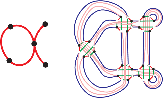
However, the contrary, given a gem to find by a polynomial algorithm a blackboard framed link inducing the same 3D-space is, as far as we know, an untouched problem in the literature. Figure 1.67 shows this computational gap as a red arrow. The reason why it is desirable to have this arrow in black stems from the fact that the quantum invariants are not computable from a triangulation or gem based presentation of 3D-spaces. The two languages, triangulations and blackboard framed links have at present only a one way translation.

Trying to get this converse algorithm took a long a time of our research for this thesis. Only recently we got confident that we have succeeded. A first step in this direction was given in the paper [Lin07], where a linear algorithm to prove the Lickorish-Wallace Theorem is provided. The second part, which actually presents the blink from the gem is a joint work with S. Lins [LL07] and awaits a proper computer implementation. The first test of this implementation will be to get a blink for .
The Blink computer program
A computer program to manipulate spaces through its many possible presentations was one of our goals in this work. Indeed, a great effort was made to bring Blink to life: a program written in Java that, at this moment, has more than 800 hundred classes and more than 70000 lines of code. Today, Blink supports blinks, g-blink, BFLs and 3-gems. The idea is, in the future, to bring other possible space presentations, like special spines, into it.
To make Blink a flexible program we decided that its interface would be a Command Line Interface. It displays a prompt and the user enters a command or a script written in a language that we also name Blink. Once a command or script has been entered, the program calculates the script result and shows it to the user. The flexibility we get in this type of design is good; for example we can combine functions and easily express more complex functions.
Besides the calculation of invariants, the identification of certain structures into 3-gems (e.g. disconnecting quartets, dipoles) or into g-blinks (e.g. simplification points) one of the main characteristics of Blink is its capability of presenting drawings or diagrams for blinks, g-blink, BFLs and 3-gems. Almost all drawings on this thesis came from Blink. To get good looking and correct drawings for blinks, g-blinks and BFLs took us a long time once we didn’t know a good way of doing it. But finally we found a great solution: Tamassia’s Algorithm [Tam87].
We have implemented the following four algorithms to deal with the drawing issue. Except for the first algorithm, the other three are further fine-tuned with Bézier curves and splines techniques ([FvDFH90]) to produce rounded-drawings with curved edges.
- 1.
Coin-drawing Algorithm: this was our own first original algorithm which we implemented to correctly draw in a visible scale the whole of any plane graph. The drawing is in the interior of a disk named a coin. The coin-drawing algorithm chooses and draw a spanning tree of the graph with appropriate lengths and angles. These ensure that the remaining edges can be displayed as a path which is a line segment, an arc of circle and another line segment. This is the simplest algorithm producing the less pleasing aesthetical effect. Nevertheless, these coin-drawings are important because they were, for a long time in our work, the only general method with total visibility. Figure 1.68 presents an example of our coin drawing algorithm.

Figure 1.68: Coin drawing of - 2.
Tutte’s Barycentric Algorithm [Tut67]: we have implemented this well known algorithm that draws a -connected plane graph by choosing the external face and extending the drawing so that every interior vertex is in the barycenter of its neighbors. Frequently, it produces pleasant drawings. However it does not treat the less connected graphs which are central for our work: loops, pendant vertices and cut-vertices are of fundamental importance in blink theory. Another problem that occurs with Tutte’s based algorithm is the one of discrepant scales: some parts of the drawing are exponentially smaller that others, and simply disappear from the drawings. Despite of these disadvantages, Tutte’s algorithm works well for the majority of blinks in the set .
- 3.
Koebe, Andreev and Thurston’s Theorem on circle packing in the hyperbolic plane: beautiful drawings of plane graphs are possible to obtain from the geometry of the hyperbolic plane. Given a -connected plane graph, there exist circles centered at the vertices of the graph so that the edges are defined by the contact points of two circles. See the articles of Smith [Smi94], Stephenson [Ste03] of Collins and Stephenson [CS03] where algorithms are outlined for the case of triangulations. The Theorem yielding the circle packing was proved independently by Koebe [Koe36], Andreev [And70] and by Thurston [Thu82]. We have implemented our own version of the algorithm which works in the case of -connected graphs. However, it suffers the same disadvantages as Tutte’s Algorithm. Nevertheless, when it works it produces the nicest results. Figure 1.69 presents a blink, its BFL, the circle packing that defined the first two drawings, and the first three drawings together.

Figure 1.69: Circle packing of a 3-connected blink - 4.
Tamassia’s Algorithm [Tam87]: to embed an arbitrary plane graph with valency at most 4 in the rectilinear grid so as to minimize the number of bends. This algorithm came to our attention only at latter phase of our research. Fine-tunings of it has all the properties we needed: it correctly draws any plane graph and it does not suffer from the undesirable phenomenon of discrepant scales: all the vertices and the edges are entirely well visible. The objective of the method is to minimize (in a precisely defined mathematical way) the number of bends. The algorithm depends three times on the algorithm to compute a minimum cost-flow in a network. The essence of this algorithm is in the design of the first network. Each feasible flow in this network encodes valid “shapes” for the edges of the graph. This encoding tells, for example, that an edge has no bends or that it has one bend to the right then one bend to the left. When a minimum flow is found in this network the minimum number of bends for a valid rectilinear embedding of the given graph is found. The other two networks are used to find the lengths of the horizontal end vertical segments of the edges. In order to have Tamassia’s algorithm available, we had first to implement the minimum cost flow algorithm in its full generality via the network simplex method. We have based our implementation on the lucid exposition Chapter 19 of [Chv83] and in the (editor’s categorization) “Exceptional Paper” [GHBG77], which is the original source of the network simplex method. Tamassia’s algorithm is an unexpected application of network flow theory in its full strength. Since its publication in 1987, it has become a theoretically beautiful at the same time a practical device used on dozens of applications. Having implemented it from scratch, we had the opportunity of tailoring it to fulfill our expectations on drawing of general plane graphs. In particular, the restriction about the maximum degree 4 is easy to overcome. Finally, the use of Bézier curves and splines ([FvDFH90]) makes the drawings more pleasing aesthetically, with smaller perceptual complexity. All drawings in the Appendices are based in this algorithm.
We want to make Blink an open source project on the internet but this wasn’t done yet.
An example of Blink usage
We finish this section with an example of the usage of Blink. Here is the code:
// associates B to the g-blink with 4 parallel green edges: U[5]
B = gblink(5)
// all possible toroidal sums with B up to 24 edges
C = combineGBlinks({B},24)
// calculate representative
C = rep(C)
// remove duplicates
C = set(C)
// homology groups on all g-blink of C
HGs = hg(C)
// calculate quantum invariant on all g-blink of C up to level 4
QIs = qi(C,4)
// produces the blink drawings
db(C,cols=10,rows=4,eps="blinks.eps")
// produces the link drawings
dl(C,cols=10,rows=4,eps="links.eps")
The BFL presentation of is the first in to have two components. It is a blink with four parallel green edges. By merging with itself in all possible ways we obtain 38 representative blinks with 24 edges. These 38 blinks and their associated BFLs are shown in Figure 1.70. We calculated homology group and the quantum invariant up to level 4 of these 38 blinks. We could distinguish 24 spaces. The blinks we cannot distinguish with this experiment are: , , , , , , , .
| # | HG | r=3 | r=4 |
|---|---|---|---|
| 01 | |||
| 02 | |||
| 03 | |||
| 04 | |||
| 05 | |||
| 06 | |||
| 07 | |||
| 08 | |||
| 09 | |||
| 10 | |||
| 11 | |||
| 12 | |||
| 13 | |||
| 14 | |||
| 15 | |||
| 16 | |||
| 17 | |||
| 18 | |||
| 19 |
| # | HG | r=3 | r=4 |
|---|---|---|---|
| 20 | |||
| 21 | |||
| 22 | |||
| 23 | |||
| 24 | |||
| 25 | |||
| 26 | |||
| 27 | |||
| 28 | |||
| 29 | |||
| 30 | |||
| 31 | |||
| 32 | |||
| 33 | |||
| 34 | |||
| 35 | |||
| 36 | |||
| 37 | |||
| 38 |
Observe the curious fact that, except for the first blink, the quantum invariants at level are Gauss integers (i.e. with integers). This type of experiment is very easy to do with Blink.

Two final remarks
First. Recently we have extended the set to blinks with up to 10 edges. The number of blinks was increased from 3437 to 17948. The number of potentially prime classes increased from 487 to 1025. The number of composite classes increased from 14 to 40. We did not attempt the topological classification of the classes 10.__ using 3-gems.
Second. We have a contract with World Scientific Publisher to write a book to be co-authored by S. Lins based on the material of this thesis. The tentative title of this book: All Shapes of Spaces: a Genealogy of Closed Oriented 3-Manifolds and it should be finished by the year 2008.
The 487 potentially prime spaces in
We here present the 487 spaces that are “potentially prime” once we could not prove them composite in our tests. One thing is certain, as stated in Theorem Topological classification of g-blinks in : any prime space that can be presented as a blink with 9 edges induces the same space (modulo orientation) as one and only one of these 487 spaces. Actually there are two points where this last statement may fail: space 9.126 and space 9.199 (although they have the same HGnQI we could not find a proof of homeomorphism between g-blink and the other g-blinks in 9.126 and g-blink and the others in 9.199). All 3437 g-blinks in appears in this Appendix or in Appendix The 14 composite spaces in .

The elements of this catalogue are: (1) the space name: is a synonym for ; (2) the primality test outcome; (3) the homology group; (4) the number of g-blinks in that induces this space; (5) number of 3-gems identified in the same ts-class of the minimum 3-gem found for this space: full means that all ts-class was identified, partial means that we do not know if all ts-class was identified; (6) the minimum blink presentation for this space in set and also a minimal presentation for this space (this is always true, except for class that should be ); (7) the name of the g-blink in ; (8) its number of edges; (9) its number of blocks in the blink presentation (2-connected components); (10) its orientation compared to the orientation of the QI shown: + sign means the same and - sign means different; (11) the corresponding BFL presentation; (12) other g-blinks in the same space; (13) the code of the minimal 3-gem found for this space the code convention is defined in [Lin95]; (14) the number of handles (composition with and the number of vertices of this 3-gem); (15) the quantum invariant of this space in polar form where the angle is divided by ; (16) the name of this minimal 3-gem in the catalogue of [Lin95] when it is present in this catalogue.
The spaces that have integral quantum invariants up to level 12 are: 6.5 , 6.8, 6.18 and 8.32. The spaces that have real but not integral quantum invariant up to level 12 are 1.1, 2.1, 4.4, 6.14, 6.19, 8.58, 8.70, 8.75, 8.76, 8.81, 8.86, 8.87, 8.89, 8.100, 8.102, 8.103, 8.117, 9.23, 9.183. The remaining classes have entries with non-zero imaginary part (i.e. ).
![[Uncaptioned image]](0702057v1/catalog001.png)
![[Uncaptioned image]](0702057v1/catalog002.png)
![[Uncaptioned image]](0702057v1/catalog003.png)
![[Uncaptioned image]](0702057v1/catalog004.png)
![[Uncaptioned image]](0702057v1/catalog005.png)
![[Uncaptioned image]](0702057v1/catalog006.png)
![[Uncaptioned image]](0702057v1/catalog007.png)
![[Uncaptioned image]](0702057v1/catalog008.png)
![[Uncaptioned image]](0702057v1/catalog009.png)
![[Uncaptioned image]](0702057v1/catalog010.png)
![[Uncaptioned image]](0702057v1/catalog011.png)
![[Uncaptioned image]](0702057v1/catalog012.png)
![[Uncaptioned image]](0702057v1/catalog013.png)
![[Uncaptioned image]](0702057v1/catalog014.png)
![[Uncaptioned image]](0702057v1/catalog015.png)
![[Uncaptioned image]](0702057v1/catalog016.png)
![[Uncaptioned image]](0702057v1/catalog017.png)
![[Uncaptioned image]](0702057v1/catalog018.png)
![[Uncaptioned image]](0702057v1/catalog019.png)
![[Uncaptioned image]](0702057v1/catalog020.png)
![[Uncaptioned image]](0702057v1/catalog021.png)
![[Uncaptioned image]](0702057v1/catalog022.png)
![[Uncaptioned image]](0702057v1/catalog023.png)
![[Uncaptioned image]](0702057v1/catalog024.png)
![[Uncaptioned image]](0702057v1/catalog025.png)
![[Uncaptioned image]](0702057v1/catalog026.png)
![[Uncaptioned image]](0702057v1/catalog027.png)
![[Uncaptioned image]](0702057v1/catalog028.png)
![[Uncaptioned image]](0702057v1/catalog029.png)
![[Uncaptioned image]](0702057v1/catalog030.png)
![[Uncaptioned image]](0702057v1/catalog031.png)
![[Uncaptioned image]](0702057v1/catalog032.png)
![[Uncaptioned image]](0702057v1/catalog033.png)
![[Uncaptioned image]](0702057v1/catalog034.png)
![[Uncaptioned image]](0702057v1/catalog035.png)
![[Uncaptioned image]](0702057v1/catalog036.png)
![[Uncaptioned image]](0702057v1/catalog037.png)
![[Uncaptioned image]](0702057v1/catalog038.png)
![[Uncaptioned image]](0702057v1/catalog039.png)
![[Uncaptioned image]](0702057v1/catalog040.png)
![[Uncaptioned image]](0702057v1/catalog041.png)
![[Uncaptioned image]](0702057v1/catalog042.png)
![[Uncaptioned image]](0702057v1/catalog043.png)
![[Uncaptioned image]](0702057v1/catalog044.png)
![[Uncaptioned image]](0702057v1/catalog045.png)
![[Uncaptioned image]](0702057v1/catalog046.png)
![[Uncaptioned image]](0702057v1/catalog047.png)
![[Uncaptioned image]](0702057v1/catalog048.png)
![[Uncaptioned image]](0702057v1/catalog049.png)
![[Uncaptioned image]](0702057v1/catalog050.png)
![[Uncaptioned image]](0702057v1/catalog051.png)
![[Uncaptioned image]](0702057v1/catalog052.png)
![[Uncaptioned image]](0702057v1/catalog053.png)
![[Uncaptioned image]](0702057v1/catalog054.png)
![[Uncaptioned image]](0702057v1/catalog055.png)
![[Uncaptioned image]](0702057v1/catalog056.png)
![[Uncaptioned image]](0702057v1/catalog057.png)
![[Uncaptioned image]](0702057v1/catalog058.png)
![[Uncaptioned image]](0702057v1/catalog059.png)
![[Uncaptioned image]](0702057v1/catalog060.png)
![[Uncaptioned image]](0702057v1/catalog061.png)
![[Uncaptioned image]](0702057v1/catalog062.png)
![[Uncaptioned image]](0702057v1/catalog063.png)
![[Uncaptioned image]](0702057v1/catalog064.png)
![[Uncaptioned image]](0702057v1/catalog065.png)
![[Uncaptioned image]](0702057v1/catalog066.png)
![[Uncaptioned image]](0702057v1/catalog067.png)
![[Uncaptioned image]](0702057v1/catalog068.png)
![[Uncaptioned image]](0702057v1/catalog069.png)
![[Uncaptioned image]](0702057v1/catalog070.png)
![[Uncaptioned image]](0702057v1/catalog071.png)
![[Uncaptioned image]](0702057v1/catalog072.png)
![[Uncaptioned image]](0702057v1/catalog073.png)
![[Uncaptioned image]](0702057v1/catalog074.png)
![[Uncaptioned image]](0702057v1/catalog075.png)
![[Uncaptioned image]](0702057v1/catalog076.png)
![[Uncaptioned image]](0702057v1/catalog077.png)
![[Uncaptioned image]](0702057v1/catalog078.png)
![[Uncaptioned image]](0702057v1/catalog079.png)
![[Uncaptioned image]](0702057v1/catalog080.png)
![[Uncaptioned image]](0702057v1/catalog081.png)
![[Uncaptioned image]](0702057v1/catalog082.png)
![[Uncaptioned image]](0702057v1/catalog083.png)
![[Uncaptioned image]](0702057v1/catalog084.png)
![[Uncaptioned image]](0702057v1/catalog085.png)
![[Uncaptioned image]](0702057v1/catalog086.png)
![[Uncaptioned image]](0702057v1/catalog087.png)
![[Uncaptioned image]](0702057v1/catalog088.png)
![[Uncaptioned image]](0702057v1/catalog089.png)
![[Uncaptioned image]](0702057v1/catalog090.png)
![[Uncaptioned image]](0702057v1/catalog091.png)
![[Uncaptioned image]](0702057v1/catalog092.png)
![[Uncaptioned image]](0702057v1/catalog093.png)
![[Uncaptioned image]](0702057v1/catalog094.png)
![[Uncaptioned image]](0702057v1/catalog095.png)
![[Uncaptioned image]](0702057v1/catalog096.png)
![[Uncaptioned image]](0702057v1/catalog097.png)
![[Uncaptioned image]](0702057v1/catalog098.png)
![[Uncaptioned image]](0702057v1/catalog099.png)
![[Uncaptioned image]](0702057v1/catalog100.png)
![[Uncaptioned image]](0702057v1/catalog101.png)
The 14 composite spaces in
We here present the 14 spaces induced from g-blinks in . Their “connected sum” details: what prime spaces compose to them are shown in Chapter Computational experiments and results. The elements of this presentation are the same as the explained in Appendix The 487 potentially prime spaces in .
![[Uncaptioned image]](0702057v1/compcatalog001.png)
![[Uncaptioned image]](0702057v1/compcatalog002.png)
![[Uncaptioned image]](0702057v1/compcatalog003.png)
Simple 3-connected monochromatic blinks up to 16 edges
We here present all simple 3-connected green blinks with edges divided in 381 HGnQI classes. The quantum invariant was calculated up to level for each of these blinks. There are left 11 uncertainties: 14.24t, 15.16t, 15.19t, 15.22t, 16.42t, 16.56t, 16.141t, 16.142t, 16.149t, 16.233t. Except for these classes the other 370 consisted of only one blink (or the two orientations of the same space). This fact suggests that if and are two different simple 3-connected monochromatic blinks, that do not form a trivial pair (trivially induce the same space), then they probably induce different spaces. Are the 11 uncertainties examples of non-trivial pairs?
![[Uncaptioned image]](0702057v1/con3catalog001.png)
![[Uncaptioned image]](0702057v1/con3catalog002.png)
![[Uncaptioned image]](0702057v1/con3catalog003.png)
![[Uncaptioned image]](0702057v1/con3catalog004.png)
![[Uncaptioned image]](0702057v1/con3catalog005.png)
![[Uncaptioned image]](0702057v1/con3catalog006.png)
![[Uncaptioned image]](0702057v1/con3catalog007.png)
![[Uncaptioned image]](0702057v1/con3catalog008.png)
![[Uncaptioned image]](0702057v1/con3catalog009.png)
![[Uncaptioned image]](0702057v1/con3catalog010.png)
![[Uncaptioned image]](0702057v1/con3catalog011.png)
![[Uncaptioned image]](0702057v1/con3catalog012.png)
![[Uncaptioned image]](0702057v1/con3catalog013.png)
![[Uncaptioned image]](0702057v1/con3catalog014.png)
![[Uncaptioned image]](0702057v1/con3catalog015.png)
![[Uncaptioned image]](0702057v1/con3catalog016.png)
![[Uncaptioned image]](0702057v1/con3catalog017.png)
![[Uncaptioned image]](0702057v1/con3catalog018.png)
![[Uncaptioned image]](0702057v1/con3catalog019.png)
![[Uncaptioned image]](0702057v1/con3catalog020.png)
![[Uncaptioned image]](0702057v1/con3catalog021.png)
![[Uncaptioned image]](0702057v1/con3catalog022.png)
![[Uncaptioned image]](0702057v1/con3catalog023.png)
![[Uncaptioned image]](0702057v1/con3catalog024.png)
![[Uncaptioned image]](0702057v1/con3catalog025.png)
![[Uncaptioned image]](0702057v1/con3catalog026.png)
![[Uncaptioned image]](0702057v1/con3catalog027.png)
![[Uncaptioned image]](0702057v1/con3catalog028.png)
![[Uncaptioned image]](0702057v1/con3catalog029.png)
![[Uncaptioned image]](0702057v1/con3catalog030.png)
![[Uncaptioned image]](0702057v1/con3catalog031.png)
![[Uncaptioned image]](0702057v1/con3catalog032.png)
![[Uncaptioned image]](0702057v1/con3catalog033.png)
![[Uncaptioned image]](0702057v1/con3catalog034.png)
![[Uncaptioned image]](0702057v1/con3catalog035.png)
![[Uncaptioned image]](0702057v1/con3catalog036.png)
![[Uncaptioned image]](0702057v1/con3catalog037.png)
![[Uncaptioned image]](0702057v1/con3catalog038.png)
![[Uncaptioned image]](0702057v1/con3catalog039.png)
References
- [And70] E. M. Andreev. Convex polyhedra in Lobatchevski space. Math. USSR Sbornik, 10:413–440, 1970.
- [BM76] J. A. Bondy and U. S. R. Murty. Graph Theory with Applications. American Elsevier Publishing Co., Inc., 1976.
- [CC06] M. R. Casali and P. Cristofori. A catalogue of orientable 3-manifolds triangulated by 30 coloured tetrahedra. arXiv:math.GT/0606359 v1, 2006.
- [Chv83] Vasek Chvátal. Linear programming. Freeman and Company, 1983.
- [CS03] Charles R. Collins and Keneth Stepheson. A circle packing algorithm. Comp. Geom., 25:233–256, 2003.
- [Dra98] Interactive Topological Drawing. Robert Glenn Scharein. PhD thesis, The University of Bristish Columbia, 1998.
- [FR79] R. A. Fenn and C. P. Rourke. On kirby’s calculus of links. Topology, 18:1–15, 1979.
- [FvDFH90] J. D. Foley, A. van Dam, S. K. Feiner, and J.F. Hughes. Computer grpahics: principles and practice. Addison-Wesley, 1990.
- [GHBG77] G. G. Brown G. H. Bradley and G. W. Graves. Design and implementation of large scale primal transshipment algorithms. Management Science, 24:1–34, 1977.
- [Hem76] J. Hempel. 3-Manifolds. Princeton University Press, 1976.
- [Kau87] Louis H. Kauffman. On knots. Number 115 in Annals of Mathematics Studies Number. Princeton University Press, 1987.
- [Kau91] L. H. Kauffman. Knots and physics. World Scientific, 1991.
- [Kir78] Robion Kirby. A calculus of framed links in . Invent. Math., 45:35–56, 1978.
- [KL94] Louis H. Kauffman and Sóstenes Lins. Temperley-Lieb Recoupling Theory and Invariants of 3-Manifolds (AM-134). Princeton University Press, 1994.
- [Koe36] Paul Koebe. Kontactprobleme der Konformen Abilldung. Ber. Sächs. Akad. Wiss. Leipzig, Math.-Phiys KL, 88:141–164, 1936.
- [Lic62] W. B. R. Lickorish. A representation of orientable, combinatorial 3-manifolds. Annals of Mathematics, 76:531–540, 1962.
- [Lin82] Sóstenes Lins. Graph-encoded maps. J. Comb. Theory, Ser. B, 32(2):171–181, 1982.
- [Lin95] Sóstenes Lins. Gems, Computers and Attractors for 3-Manifolds, volume 5 of Series on Knots and Everything. World Scientific Publishing Company, 1995.
- [Lin07] Sóstenes Lins. Combinatorial dehn-lickorish twists and framed link presentations of 3-manifolds revisited. submitted to the Journal of Knot Theory and its Ramifications, 2007.
- [LL07] Lauro Lins and Sóstenes Lins. From triangulations to framed link presentations of 3d-spaces: a polynomial algorithm. under preparation, 2007.
- [Mat03] S. Matveev. Algorithmic topology and classification of 3-manifolds, volume 9 of Series Algorithms and Computation in Mathematics. Springer, 2003.
- [Moi52] E. E. Moise. Affine structures in 3-manifolds. Ann. Math., 56:96–114, 1952.
- [Rei48] K. Reidemeister. Knotentheorie. Chelsea, New York (1948).
- [Rol76] Dale Rolfsen. Knots and Links. AMS Chelsea Pub., 1976.
- [RT91] N. Y. Reshetikhin and V. Turaev. Invariants of threee manifolds via link polynomials and quantum groups. Invent. Math., 103:547–597, 1991.
- [Smi94] Warren D. Smith. Accurate circle configurations and numerical conformal mapping in polynomial time. Preprint tyset on June 14, 1994, available in the Internet, 50:1376–1388, 1994.
- [Ste03] Keneth Stepheson. Circle packing: a mathematical tale. Notices of the AMS, 50:1376–13886, 2003.
- [Sti80] John Stillwell. Classical Topology and Combinatorial Group Theory. Springer, 1 edition, 1980.
- [Sti97] John Stillwell. Numbers and Geometry. Springer, 1997.
- [Tam87] Roberto Tamassia. On embedding a graph in the grid with the minimum number of bends. Siam J. Comp., 16:421–444, 1987.
- [Thu82] William Thurston. The geometry and topology of 3-manifolds. Princeton University Notes, 1982.
- [Tut67] William. T. Tutte. How to draw a graph. Proc. London Math. Soc., 13:743–768, 1967.
- [VINK] O. Y. Viro, O. A. Ivanov, N. Y. Netsvetaev, and V. M. Kharlamov. Elementary Topology A First Course Textbook in Problems. in preparation.
- [Wal60] A. H. Wallace. Modifications and cobounding manifolds. Canad. J. Math, 12:503–528, 1960.
- [Wik06a] Wikipedia. Seven bridges of königsberg — wikipedia, the free encyclopedia, 2006. [Online; accessed 9-October-2006].
- [Wik06b] Wikipedia. Topology — wikipedia, the free encyclopedia, 2006. [Online; accessed 9-October-2006].
- [Wit89] Edward Witten. Quantum field theory and the jones polynomial. Commun. Math. Phys., 121:351, 1989.
- [WN99] Laurence A. Wolsey and George L. Nemhauser. Integer and Combinatorial Optimization. Wiley-Interscience, 1999.
*