A Presentation for $Aut(F_{n})$

We will apply Theorem  2 to a certain subcomplex of the spine of Auter space. The spine of Auter space is a contractible simplicial complex on which $Aut(F_{n})$ acts with finite stabilizers and finite quotient. For full details on the construction of Auter space, we refer to [4].

A vertex in the spine of Auter space is a connected, basepointed graph $\Gamma$ together with an isomorphism $g\colon\pi_{1}(\Gamma)\to F_{n}$, called a marking. (Note: often in the literature the marking goes in the other direction). We require all vertices of $\Gamma$ to have valence at least three, and we also assume that $\Gamma$ has no separating edges. One can describe the marking $g$ by labeling certain edges of $\Gamma$ as follows. Choose a maximal tree in $\Gamma$. The edges not in this maximal tree form a natural basis for the fundamental group $\pi_{1}(\Gamma)$. Orient each of these, and label them by their images in $F_{n}$. This description depends on the choice of maximal tree; for instance the labeled graphs in Figure 1 represent the same vertex.

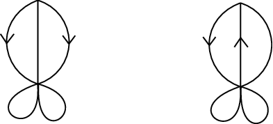
Two marked graphs span an edge in the spine if one can be obtained from the other by collapsing a set of edges (this is called a forest collapse). A set of $k+1$ vertices spans a $k$-simplex if each pair of vertices spans an edge.

The group $Aut(F_{n})$ acts on Auter space on the left by $\alpha\cdot(g,\Gamma)=(\alpha\circ g,\Gamma)$. This is represented on a labeled graph by applying $\alpha$ to the edge-labels. Figure 2 shows the results of applying $\eta$ to the graph from Figure 1. Note that this is the same marked graph, so that $\eta$ fixes this vertex of the spine.

The degree of a graph is defined to be $2n$ minus the valence of the basepoint. The only graph of degree 0 is a rose, and the only graph of degree 1 is the graph underlying the marked graph in Figure 1. There are five different graphs of degree 2.

A forest collapse cannot increase degree, so the vertices of degree at most $i$ span a subcomplex $K_{i}$ of the spine. Hatcher and Vogtmann proved that the subcomplexes $K_{i}$ act like “skeleta” for the spine of Auter space:

In particular, the subcomplex $K_{2}$ spanned by graphs of degree at most 2 is a simply-connected 2-complex.

The quotient of $K_{2}$ by the action of $Aut(F_{n})$ was computed in [4]. For $n\geq 4$, this quotient has seven vertices, thirteen edges and seven triangles. Figure 3 shows a lift of these simplices to $K_{2}$ for $n=4.$ For $n>4$, the picture is the same except one must add $n-4$ loops at the basepoint. The darkest edges represent a choice of tree $\mathcal{T}$ lifting a maximal tree in the 1-skeleton of $K_{2}/Aut(F_{n})$, and the lighter solid edges represent the additional edges in $\mathcal{E}$. For $n=3$, the picture is the same except that the backmost triangle is missing and every remaining graph has one fewer loop at the basepoint. For $n=2$, there are only the three leftmost triangles and every remaining graph has two fewer loops at the basepoint.

We will use the labels in Figure 3 to refer to the vertices of $\mathcal{T}$, and we will denote by $W_{n-i}$ the subgroup of $W_{n}$ which permutes and inverts the last $n-i$ generators.

The stabilizer of a vertex in the spine of Auter space can be identified with the automorphism group of the marked combinatorial graph associated to that vertex [8]. We compute:

$G_{0}=stab(v_{0})=W_{n}$.

$G_{1}=stab(v_{1})=\Sigma_{3}\times W_{n-2}$, where $\Sigma_{3}$ is the symmetric group on the three vertical edges, which is generated by $\sigma_{12}$ and $\eta$.

$G_{4}=stab(v_{4})=(\mathbb{Z}_{2}\times\mathbb{Z}_{2})\times W_{n-2}$. Here one $\mathbb{Z}_{2}$ is generated by $\sigma_{12}$ and the other $\mathbb{Z}_{2}$ is generated by $\tau_{1}\tau_{2}$.

Since $v_{3}=\eta v_{4}$, $G_{3}=stab(v_{3})=\eta G_{4}\eta$, which is generated by $\eta\tau_{1}\tau_{2}\eta$ and $\eta\sigma_{12}\eta$.

$G_{2}=stab(v_{2})=(\mathbb{Z}_{2}\times\mathbb{Z}_{2})\times W_{n-2}$. The first $\mathbb{Z}_{2}$ is generated by $\eta\tau_{1}\tau_{2}\eta$ and the second by $\tau_{1}$.

$G_{7}=stab(v_{7})=D_{8}\times W_{n-3}$, where $D_{8}$ is the dihedral group generated by $\eta\sigma_{12}\eta$ and $\tau_{2}\sigma_{13}$.

$G_{6}=stab(v_{6})=D_{8}\times W_{n-3}$. Here $D_{8}$ is the dihedral group generated by $\sigma_{12}$ and $\eta\sigma_{13}\tau_{2}\eta$. Note that $G_{7}=\eta G_{6}\eta$, since $v_{7}=\eta v_{6}$.

$G_{5}=stab(v_{5})=\Sigma_{4}\times W_{n-3}$. The symmetric group $\Sigma_{4}$ corresponds to permuting the edges which are not loops and is generated by the involutions $\sigma_{12},\eta\sigma_{13}\tau_{2}\eta$ and $\sigma_{23}.$ Note that $G_{6}$ is a subgroup of $G_{5}$.

$G_{8}=stab(v_{8})=((\Sigma_{3}\times\Sigma_{3})\rtimes\mathbb{Z}_{2})\times W_{n-4}$. The factor $\mathbb{Z}_{2}$ is generated by $\omega=\sigma_{13}\sigma_{24}$, the first $\Sigma_{3}$ is equal to $G_{1}$ and the second $\Sigma_{3}$ is $\omega G_{1}\omega$ .

By Brown’s theorem, $Aut(F_{n})$ is generated by the vertex stabilizers $G_{i}$ corresponding to vertices of $\mathcal{T}$, i.e. $G_{0},G_{1},G_{2},G_{3},G_{5},G_{6}$ and $G_{8}$, together with a generator $t_{e}$ for each of the 13 edges of $\mathcal{E}$. We denote the oriented edge from $v_{i}$ to $v_{j}$ by $e_{ij}$.

If $e\in\mathcal{T}$ (i.e. $e=e_{0k}$ for $k\in\{3,6,8\}$ or $e_{k0}$ for $k\in\{1,2,5\}$), then the tree relations set $t_{e}=1$.

If all edges of a triangle $\Delta$ are in $\mathcal{E}$ and two of the edges lie in $\mathcal{T}$, then $h=1$ and $g_{e}=1$ for all edges in the boundary of $\Delta$, so the face relation associated to $\Delta$ reduces to $t_{e}=1$ for the third edge $e$. We now have $t_{e}=1$ for all edges except $e_{04}$ and $e_{07}$.

The only faces which do not have two edges in $\mathcal{T}$ are the shaded faces labeled $\Delta_{104}$ and $\Delta_{107}$ in Figure 3. The boundary of $\Delta_{107}$ is given by the edge-path loop $e_{10}e_{07}e_{71}$. The first edge $e_{10}$ is in $\mathcal{T}$, giving $h_{10}=1$ and $g_{e_{10}}=1$, so $g_{10}=1$. The second edge $e_{07}$ is in $\mathcal{E}$, so $h_{07}=1$; this edge has $t(e_{07})=v_{7}=\eta v_{6}$, so $w(e_{07})=v_{6}$ and $g_{e_{07}}=\eta$, giving $g_{07}=\eta$. The last edge $e_{71}$ is equal to $\eta e_{61}$, and $e_{61}\in\mathcal{E}$. Thus $h_{71}=1$, and $g_{e_{71}}=1$, giving $g_{71}=1$. We have $g_{10}g_{07}g_{71}=\eta$, and the relation associated to ${\Delta_{107}}$ is now

which reduces to $t_{e_{07}}=\eta$. An identical calculation for $\Delta_{104}$ gives $t_{e_{04}}=\eta$, since $\eta v_{4}=v_{3}$.

The edge relations identify generators of the vertex groups with the appropriate products of the $\tau_{i}$, $\sigma_{ij}$ and $\eta$. If $e\in\mathcal{T}$, the edge relations identify all of the generators written as products of $\tau_{i}$ and $\sigma_{ij}$ in our descriptions of the $G_{i}$ with the corresponding elements of $G_{0}=W_{n}$; in particular, the subgroups $W_{n-k}$ of the stabilizers are all identified with the corresponding subgroup of $G_{0}$. The edge relation associated to $e_{04}$ identifies the generators of $G_{3}$ with $\eta\tau_{1}\tau_{2}\eta$ and $\eta\sigma_{12}\eta$, since $\eta v_{4}=v_{3}$. The edge relation associated to $e_{23}$ then identifies the first generator of $G_{2}$ with $\eta\tau_{1}\tau_{2}\eta$.

The edge relation associated to $e_{07}$ identifies the second generator of $G_{6}$ with $\eta\tau_{2}\sigma_{13}\eta$, since $\eta v_{7}=v_{6}$. The edge relation associated to $e_{56}$ identifies $G_{6}$ with the subgroup of $G_{5}$ generated by $\eta\tau_{2}\sigma_{13}\eta$ and $\sigma_{12}$.

The edge relation associated to $e_{18}$ identifies the first $\Sigma_{3}$ with the corresponding $\Sigma_{3}$ subgroup of $G_{1}$.

We will not list the relations in $G_{0}=W_{n}$. The relations in $G_{1}$ which do not come from $G_{0}$ are those involving $\eta$, i.e.

Since $G_{3}=\eta G_{4}\eta$, and $G_{4}$ is a subgroup of $W_{n}$, $G_{3}$ does not contribute any new relations. The fact that the generators of $\mathbb{Z}_{2}\times\mathbb{Z}_{2}\leq G_{2}$ commute contributes the relation $(\eta\tau_{1}\tau_{2}\eta\tau_{1})^{2}=1$, which looks a little nicer if we conjugate by $\eta\tau_{1}$:

In the dihedral group $D_{8}\leq G_{6}$, the fact that the product of our generators has order 4 contributes a new relation

The symmetric group $\Sigma_{4}\leq G_{5}$ is generated by the involutions $\sigma_{12},\sigma_{23}$ and $\phi=\eta\sigma_{13}\tau_{2}\eta$, with relations $(\sigma_{12}\sigma_{13})^{3}=1,(\sigma_{12}\phi)^{4}=1$ and finally $\sigma_{12}\phi\sigma_{12}(\sigma_{23}\phi)^{2}=1$. The first relation comes from $G_{0}$ and the second from $G_{6}$, so $G_{5}$ adds only the third relation, i.e.

The fact that the two copies of $\Sigma_{3}$ which are contained in $G_{8}$ commute produces the relation $(\sigma_{14}\sigma_{23}\eta\sigma_{23}\sigma_{14}\eta)^{2}=1$, i.e.

All other relations in $G_{8}$ are consequences of this and relations in $G_{0}$ and $G_{1}$; for example the fact that $\eta\sigma_{12}\eta=\sigma_{34}$ commutes with $\eta$ is a consequence of relations already accounted for in $G_{1}$.

This completes the proof of Theorem 1 and its corollaries.

References

- [1] M. R. Bridson and A. Haefliger, Metric spaces of non-positive curvature, Grundlehren der Mathematischen Wissenschaften [Fundamental Principles of Mathematical Sciences], vol. 319, Springer-Verlag, Berlin, 1999.
- [2] K. S. Brown, Presentation for Groups Acting on Simply-Connected Complexes, Journal of Pure and Applied Algebra 32 (1984), 1–10.
- [3] S. M. Gersten, A presentation for the special automorphism group of a free group, J. Pure Appl. Algebra 33(3) (1984), 269–279.
- [4] A. Hatcher and K. Vogtmann, Cerf theory for graphs, J. London Math. Soc. (2) 58(3) (1998), 633–655.
- [5] J. McCool, A presentation for the automorphism group of a free group of finite rank, J. London Math. Soc. (2) 8 (1974), 259–266.
- [6] J. Nielsen, Die isomorphismengruppe der freien Gruppen, Math. Ann. 91 (1924), 169–209.
- [7] B.H. Neumann, Die Automorphismengruppe der freien Gruppen, Math. Ann. 107 (1932), 367–386.
- [8] K. Vogtmann, Automorphisms of Free Groups and Outer Space, Geometriae Dedicata 94 (2002), 1–31.
- [9] P. Zucca, On the -generation of the automorphism groups of free groups, Istit. Lombardo Accad. Sci. Lett. Rend. A 131 (1997),179–188.