Inverse Boundary Spectral Problem for Riemannian Polyhedra
We consider an admissible Riemannian polyhedron with piece-wise smooth boundary. The associated Laplace defines the boundary spectral data as the set of eigenvalues and restrictions to the boundary of the corresponding eigenfunctions. In this paper we prove that the boundary spectral data prescribed on an open subset of the polyhedron boundary determine the admissible Riemannian polyhedron uniquely.
1 Introduction
Recent years have seen some very significant achievements in the study of inverse boundary-value problems in a single component body. Mathematically such body is described by a PDE or a system of PDE’s with relatively smooth coefficients. Starting from the pioneering works [8] and [43], inverse boundary-value problems were solved, at least on the level of uniqueness and sometimes conditional stability, for a wide range of scalar inverse problems, both isotropic and anisotropic, see e.g. [5], [9], [10], [21], [24], [30], [31], [32], [33], [36], [39], [42] for a far from complete list of references, with further references in monographs [18] or [22]. Moreover, for such media there appeared a number of important results in the study of the inverse boundary-value problems for systems of PDE’s corresponding to physically important models of electromagnetism, elasticity and Dirac equations, see e.g. [19], [28], [29], [34], [35], [37], [38].
Much less is known, however, about the inverse boundary-value problems for a multicomponent medium. Mathematically, such medium is described by PDE or system of PDE’s with piece-wise smooth coefficients with different subdomains of the regularity of coefficients corresponding to different components of the medium. Clearly, the study of inverse problems for the multicomponent media is of substantial importance for practical applications. Imagine, for example, a human body with bones, muscle tissue, lungs, etc. each of those having distinctive values of material parameters, or an upper crust of the Earth which is a composition of clay, sand, rock, oil, water, etc. A complete answer to the inverse boundary problems in a multicomponent medium, at least when the data are measured on the whole boundary, is obtained only for the two-dimensional case. Namely, it was shown in [3], [4] that the Calderon inverse boundary problem in the 2D case has a unique solution in the class of coefficients. Clearly, these results cover also the case of a multicomponent medium. In higher dimensions, the results are restricted mainly to the inverse obstacle problem. In these problems the goal is to find a shape of an inclusion inside a given medium which parameters are known a priori. In the case when parameters of a medium and/or inclusion are unknown they are assumed to be homogeneous throughout each component, see e.g. [2], [15], [16], [17], [27]. Having said so, we should note that there exist powerful methods to find singularities for coefficients of lower order, see e.g. [12].
This paper is devoted to the study of the inverse boundary spectral problem for the Laplace operator in a multicomponent medium. To be more precise, we assume that the domain occupied by the medium consists of a finite number of subdomains with piece-wise smooth boundaries between them. The metric tensor in each subdomain is smooth but does have jump singularity across the interfaces, i.e. the boundaries between adjacent subdomains. Adding proper transmission conditions across the interfaces and boundary conditions on the domain’s boundary, defines a Laplace operator which, from the spectral point of view, has effectively the same properties as the Laplace operator in a single component medium. Mathematically, the considered medium may be described as a Riemannian polyhedron. Leaving exact definitions of an appropriate Riemannian polyhedron to the next section, imagine an dimensional simplicial complex where simpleces can be glued together, pairwise, along their dimensional faces which we continue to call interfaces (sometimes interfaces). Imagine now that each simplex has its own smooth metric which, in principle, may have jumps across interfaces between adjacent simpleces. This, together with some additional geometric/combinatoric conditions described in section 2, defines a Riemannian polyhedron . Starting from the corresponding Dirichlet form on functions and using standard methods of spectral theory, the Laplace operator with Neumann boundary conditions, , is then well-defined in . Denote by the set of all eigenvalues, counting multiplicity, and corresponding orthonormal eigenfunctions of . Let be open.
Definition 1.1
The collection is called the (local) boundary spectral data (LBSD) of the Riemannian polyhedron .
Let now and be two Riemannian polyhedra with LBSD and , correspondingly.
Definition 1.2
LBSD for and are equivalent if
- 1.
and are homeomorphic, ;
- 2.
- 3.
If has multiplicity , i.e. , then there is an unitary matrix such that
We can now formulate the main result of the paper:
Theorem 1.3
Let and be two admissible Riemannian polyhedra. Let, in addition, the metric tensors and do have jumps across all interfaces in and , correspondingly. Assume that LBSD and are equivalent. Then and are isometric.
Let us make some comments on this theorem:
- 1.
If is an dimensional simplex of with a smooth metric , then determines an inner metric on any dimensional, , simplex of which lies in (here and later we assume each simplex to be close). In particular, any interface of belongs to two adjacent simpleces, which we often denote in such case and , and therefore, has two different metric tensors and . By a metric tensor having a jump singularity across we mean that, for any ,
This assumption is of a technical nature and, in section 6 we will significantly weaken it.
- 2.
As shown in section 2, any Riemannian polyhedron has a natural structure of a metric space. The isometry of and is understood with respect to these metric structures.
- 3.
The boundary of a Riemannian polyhedron is itself a dimensional Riemannian polyhedron, probably disconnected. As are open subsets of , by reducing them if necessary we assume that and are open subsets of some dimensional simplex of , correspondingly. In the future, we will always assume this condition to be true.
The plan of the paper is as follows: In section 2 we provide some preliminary material on geometry of Riemannian polyhedra and properties of the Laplace operator on them. Section 3 is devoted to the description and some properties of the non-stationary Gaussian beams on a Riemannian polyhedron. We prove Theorem 1.3 in sections 4 and 5. The last section 6 is devoted to some generalizations and open questions.
2 Preliminary constructions
2.1 Admissible Riemannian polyhedron
In this section we will introduce, following mainly [11] and [7], an admissible Riemannian polyhedron which is the main object of the paper. We start with a closed dimensional finite simplicial complex
where are closed dimensional simpleces of , with standing for the interior of which is an open subset of . We assume that is dimensionally homogeneous, i.e. any simplex, , of is contained in at least one . We assume also that any dimensional simplex belongs either to two different simpleces, and , which in this case we will often denote by and , or to only one simplex . In the former case we call an interface (sometimes dimensional interface) between and , in the latter case we call a boundary simplex with simpleces having this property forming the boundary . We denote by the skeleton of which consists of all simpleces of . Clearly, . We use notations
Following [11], we assume that is chainable, i.e. is path connected, see Fig. 1.

Assume now that each simplex is equipped with a smooth (up to ) Riemannian metric , i.e. is a smooth Riemannian manifold with a piecewise smooth boundary. This makes it possible to introduce the arclength for admissible paths . We call a path admissible if is a (relatively) open subset of of full measure and, if is in some simplex , then is piecewise smooth. Naturally, the arclength of the path between and is taken as
| (1) |
where are, for example, baricentric coordinates in . As consists of at most a countable number of open intervals we define
| (2) |
Next we introduce, for any , the distance, ,
where infenum is taken over all admissible paths connecting and . This makes into a metric space with its metric topology being the same as the topology of a simplicial complex, see [11].
Definition 2.1
is an admissible Riemannian polyhedron if, for any ,
where run over the subset of admissible paths between and such that
As is finite, the above condition is independent of a particular choice of metric .
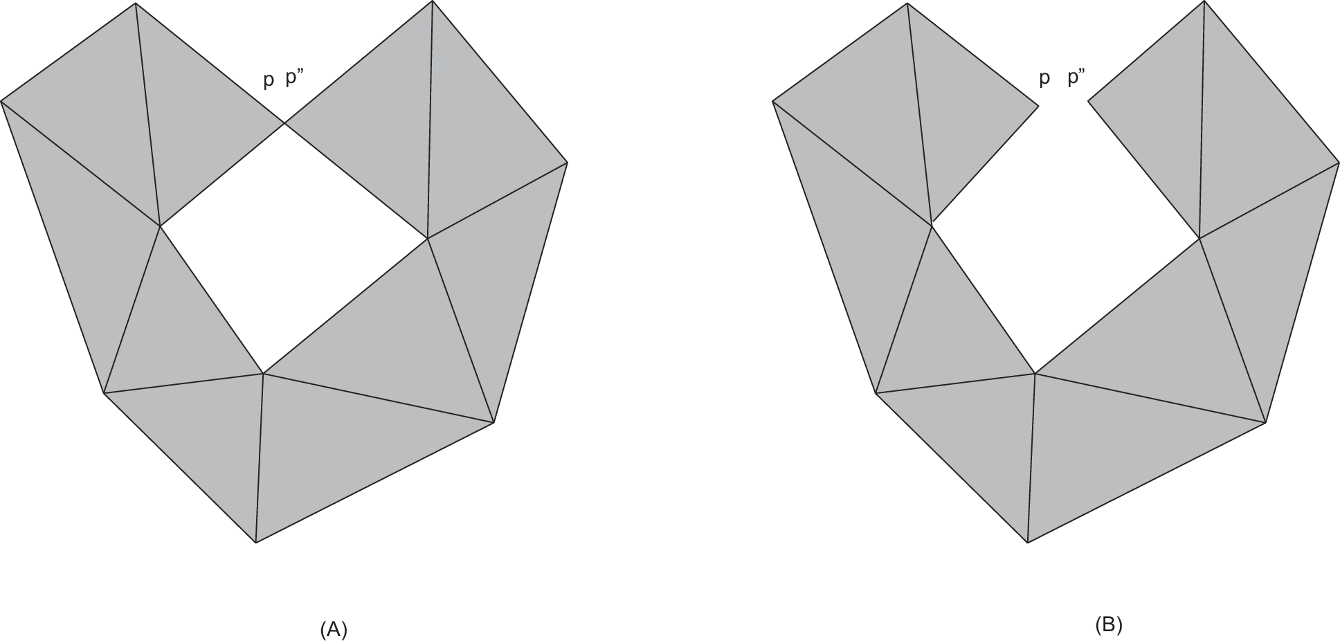
2.2 Boundary normal and interface coordinates
In addition to the baricentric coordinates in any , we will often use boundary normal or interface coordinates associated with subsimpleces of .
Let first be a boundary dimensional simplex with its dimensional interior denoted by . We introduce boundary normal coordinates in an relatively open subset as
Here , and we assume that there is a unique with , such that lies on the normal geodesic to , and . If are some (local) coordinates on , e.g. baricentric coordinates, then .
Let now be an interface between simpleces and . Let be relatively open subsets of with the nearest point on lying on such that . Denote by the boundary normal coordinates in , where are some local coordinates on , e.g. baricentric coordinates with respect to or . We introduce the interface coordinates on :
Then the metric element in these coordinates takes the form,
| (3) |
Throughout the paper we assume that the following condition takes place:
Condition 2.2
For any interface and any point on , the metric tensor has a jump singularity at .
2.3 Laplace operator
Let be the Sobolev space of functions such that and, for any interface between and ,
The inner product on determines the closed non-negative Dirichlet form,
By the standard technique of the theory of quadratic forms, the form determines a self-adjoint operator in , namely, the Laplace operator with Neumann boundary condition, . The domain is defined by
| (4) |
where is arbitrary. Analysing condition (4), we see that if and, on any interface ,
| (5) |
where .
As, due to the finiteness of , the embedding of into is compact, the spectrum of is pure discrete,
with the corresponding basis of orthonormal eigenfunctions to be denoted by . Standard considerations, see e.g. [10] or [44] show that distinguish points in , i.e. for , there is with . Moreover,
Proposition 2.3
Let be an orthonormal basis of eigenfunctions of the Laplace operator Then form local coordinates near any , i.e. there are such that form local coordinates near .
3 Gaussian Beams near interfaces
3.1 Gaussian beams on smooth manifolds
In this section we briefly recall some results on the non-stationary Gaussian beams on smooth manifolds. Their theory goes back to the pioneering works [6], [20], [41]. In our exposition we follow mainly section 2.4 of [22]. Non-stationary Gaussian beams are some (formal) solutions of the wave equation
| (6) |
which are concentrated, at each moment of time , near a point . The point moves with a unit speed along a geodesic on a smooth Riemannian manifold with being the Laplacian corresponding to Introducing a moving frame
a formal Gaussian beam has a form as a formal series
| (7) |
Here and are formal series in powers of . They are usually represented as sums of homogeneous polynomials in with coefficients depending on ,
and being homogeneous polynomials on The polynomials and are chosen so that, considered as formal series with respect to and
| (8) |
Note that exactly means that the formal series (7) satisfies formally equation (8).
The most important properties of the non-stationary Gaussian beams are:
- (a)
-
, where is the unit covector corresponding to the geodesic
- (b)
-
, where is a symmetric matrix, satisfying , for
Remark 3.1
From now on throughout this paper we use the following notations (or, ) is a generic constant, , independent of ; is defined for sufficiently large positive integers such that when .
Conditions (a) and (b) imply that decays exponentially outside an - neighborhood of . It is important to note that, starting from a formal Gaussian beam we can construct a family of solutions to the wave equation (6), which ”looks like” . To this end, we start with a finite series
| (9) |
where is a smooth cut-off function equal to near Then
By standard hyperbolic estimates there exists a solution to (6) such that
| (10) |
Moreover, if we generate a wave inside by a boundary source
| (11) |
Let be given by a formal expansion
where
| (12) |
with being homogeneous polynomials of degree with respect to . Assume that Then there is a unique formal Gaussian beam satisfying (8), and the boundary condition (11) for with some depending only on geometry of . Moreover, the corresponding geodesic starts, at from the point into the (co)diversion with geodesic starting at . We will refer to this result saying that we can guarantee a non-stationary Gaussian beam propagating transversally to by a proper choice of a boundary source (for these and other results on non-stationary Gaussian beams see e.g. [21], [22]).
3.2 Gaussian beams at interfaces
In this section we consider reflection and transmission of the non-stationary Gaussian beams from and through an dimensional interface between two -simpleces and . As our constructions will be of a local nature we can, without loss of generality, restrict them to the reflection/transmission of the Gaussian beams from a smooth interface inside a smooth manifold. These questions, for the incidence angle less then critical, were considered in detail in [26] and [40], in the latter restricted to the isotropic media. Assuming that and introducing the interface normal coordinates with corresponding to we have, for the incident Gaussian beam,
| (13) |
Here are sums of homogeneous polynomials with respect to with
with being the (co)direction of the Gaussian beam at . When it is possible to construct two formal non-stationary Gaussian beams and in and correspondingly such that
| (14) |
satisfies the wave equation (8) and transmission conditions (5). To this end we use the technique briefly described in section 3.1, which reduces the problem to finding boundary conditions of form (11), (12) for and at In turn, this is possible utilizing transmission condition (5) if Summarizing considerations of [26], we obtain the following result
Lemma 3.2
Let be a formal non-stationary Gaussian beam which hits the interface at with its (co)direction satisfying Then there are two formal Gaussian beams in and in such that the total wave satisfies the transmission condition (5). The (co)directions and of the geodesics, corresponding to and satisfy at the equation (Snell’s Law):
The main amplitude coefficients and of and are related to at by
| (15) |
where
We note that transmission condition (5) for and is understood in the formal sense. Namely, and may be expressed in the form (7) with having decomposition of form (13). Then (5) means that
and
as polynomial with respect to .
Observe that the condition implies that for almost all
When dealing with an incoming non-formal Gaussian beam (9), (10), which we will denote by , similar to the above we find and by formulae (9) with and instead of , correspondingly. Clearly, they give use to approximate transmission conditions
| (16) | |||
| (17) |
Add to a function
where are chosen so that
satisfies
| (18) | |||||
| (19) |
for . Clearly, (16), (17) imply that
Together with (18), (19), it follows from the wave equation (8) that we can modify and
with
so for . Therefore,
satisfies the wave equation (8) and coincide with for negative , more precisely, for Here is given by for and for
Remark 3.3
When is simplex in we can modify the previous construction to find the Gaussian beam reflected from The part of Lemma 3.2 related to remains valid with formula for the main term taking the form
| (20) |
Thus, by the considerations similar to the above it is possible to find solutions to the wave equation (8) which satisfy the Dirichlet boundary condition and look like a Gaussian beam.
4 First simplex
4.1
In this section we start proving the uniqueness Theorem 1.3. Recall that we are given diffeomorphic open subsets where and are boundary simpleces of simpleces We assume, after proper unitary transformations in finite-dimensional spaces corresponding to eigenvalues of higher multiplicity, that
| (21) |
where is a diffeomorphism. Our goal in this section is to prove the following result
Lemma 4.1
Let be a diffeomorphism satisfying conditions of Definition 1.2. Then there is an isometry such that
| (22) |
To prove this lemma, observe first that if and satisfy:
are regular, i.e. map into and correspondingly and provide an diffeomorphism between and and and and, in addition,
then the diffeomorphism
satisfies
Moreover, is actually an isometry between and considered as domains in and correspondingly. The proof of this fact is identical to the smooth case and is given in Section 4.4 of [22].
Assume now that and are open subsets with being isometries satisfying
| (23) |
By Proposition 1, which makes it possible to extend into an isometry which also satisfies (23).
Consider the family of all pairs of open subsets and which are isometric to each other and satisfy (23). Clearly, this family is partially ordered by induction, by the above we can consider its maximal element which we denote by with the corresponding isometry denoted by We want to show that
To proceed, recall the following result from [22], which is proven for smooth manifolds but remains valid for Riemannian polyhedra under the conditions formulated below.
Theorem 4.2
- 1.
Let (or ) be a smooth subdomain such that (or ) are known for (or for ). Assume that for
are regular. If, in addition, then these data determine uniquely where
- 2.
Let be solutions of the initial boundary value problem,
(24) Then these data determine on correspondingly. In particular, if and are isometric, with isometry satisfying (23), there is an extended isometry
with
(25) when .
4.2
Based on Theorem 4.2, we will finish the proof of Lemma 4.1. Assume, that a maximal element where without loss of generality we can take Therefore, there is a point Observe, that as is an isometry, it may be extended to the mapping Consider the following possible scenarios:
- 1.
. Denote by and by where stands for the injectivity radius of the normal coordinates of Riemannian manifold Let and satisfy Let satisfies where is a closed ball of radius centered at Taking in Theorem 4.2 to be , we see that conditions of this Theorem are satisfied for with . Therefore, can be extended to containing , which contradicts the definition of
- 2.
where is some subsimplex of Let now , where is another simplex adjacent to (if we take rather than ). As earlier, let where is the radius of injectivity of the interface normal coordinates related to (or to the boundary normal coordinates of ). Introduce as in the case 1 and take balls similar to the case 1. Consider now the non-stationary Gaussian beams on which start at at in direction close to the normal direction from to i.e. with the initial co-vector close to These Gaussian beams reflect from and return to approximately at the time Thus, for close to the total Gaussian beam in satisfies
(26) when .
On the other hand, the corresponding Gaussian beam in moves from and has no reflected part for , so that
(27) When is sufficiently small and is sufficiently large, (26), (27) contradict the second equation (25), of Theorem 4.2. As and are known we can evaluate the Fourier coefficients of and and, next,
for .
- 3.
Let now Using e.g. baricentric coordinates in we see that there are and such that if then there is a curve such that:
- (i)
-
;
- (ii)
-
, where is the arclength of between and ;
- (iii)
-
. However, we can assume that there is a unique nearest point to and, in addition,
- (iv)
-
where is an interface between and some (or );
- (v)
-
Interface (boundary) normal coordinates centered at are regular in -vicinity of .
Returning to the consideration of the case let satisfy where is defined as in the case 1. With let be a curve in described earlier. Then the diffeomorphism can be extended onto some open neighborhood of . Indeed, by the construction of the step 1, we can move recurrently along using the balls of radius By the maximality of , with satisfying
(28) Inequality (28) makes it possible to use the same considerations as in the case 2, proving that the case is possible.
We finish the section by the following
Corollary 4.3
Let where are -simpleces of and satisfy (22). If are simpleces of and correspondingly. Then is an interface if and only if is an interface.
5 Global Isometry
5.1
In this section we show that isometry on which satisfies (22) can be extended to a global isometry satisfying
| (29) | |||
We start with the following result which is a partial generalization of Theorem 4.2.
Lemma 5.1
Proof Let be smooth subdomains in and with the ”upper” part of the boundary parallel to i.e. the parts of are given by Assume, without loss of generality that , where are the injectivity radii of interface coordinates related to correspondingly. We want to show that equation (22) implies that
| (30) |
We have the following rather straightforward generalization of Tataru’s approximate controllability:
| (31) |
with a similar identity for Here is a neighborhood of in and is a solution to the initial boundary value problem
As usual this result follows immediately from observability, see e.g. Section 2.5 of [22]. To formulate the desired observability, let
where . Then in double cone
To use this we first observe that for any with and any there is a piece-wise smooth curve with and Moreover, may be chosen to cross transversally. Then we can continue by along this curve so that for
where is a small vicinity of . Indeed, this is obvious for pieces of the path lying inside either or To cross we just observe that, if on when approaching from , then by (8),
when approaching from and, therefore, can be continued by further along into and vice versa from into . Clearly, to use (5) we should assume to be sufficiently regular, however, by smoothing with respect to time we can extend it to non-smooth solutions, see e.g. [23].
This implies that for . As is arbitrary, we obtain that in .
Identity (31) makes it possible, starting from , and from , such that and , for to construct and for , see [21], Chapter 4.4 of [22]. In particular, the construction in [21], [22] imply that . Observe now that from a relatively open subdomains in respectively with being a diffeomorphism satisfying (23).
5.2 Identification of -simpleces
We have proven that, for any chain of simpleces in which are pairwise adjoint, i.e. there is an -interface between and there is a chain of -simpleces in such that and are diffeomorphic with diffeomorphism satisfying (22) (strictly speaking may depend on a chain from to ), see Fig 3.

Let us show that
- (a)
-
For any simplex there is an simplex which is diffeomorphic to with diffeomorphism satisfying (22) and, likewise, for any there is with described properties;
- (b)
-
If and are diffeomorphic with diffeomorphisms and satisfying (22) then
- (c)
-
If is diffeomorphic to and by and satisfying (22), then .
Let now be are the simpleces with used in Lemma 4.1 being their boundary subsimpleces. Then, by Lemma 4.1, there is satisfying (22). Denote by the interface between and . By Corollary 4.3, there is adjacent to with the interface such that . By Lemma 5.1, there is an isometry with . Continuing this process, we obtain an isometry , which satisfies (22).
To prove (b), let , and , . As satisfy (22), By Proposition 2.3, . As is arbitrary, on . Using the fact that distinguish points in , see Proposition 2.3, we prove property (c).
Based on properties (a)-(c) we show the following result.
Lemma 5.2
Let LBSD for the Riemannian polyhedron and be equivalent. Then
- 1.
For any in there is a unique diffeomorphism , which satisfies (22).
- 2.
is an interface between and if and only if the corresponding is an interface between and . In this case
where is the closures of the described above diffeomorphisms on ,
- 3.
The diffeomorphisms can be uniquely extended to an isometry
Here is an isometry of and considered as metric space with the distance function given in Definition 2.1.
Proof By (a)-(c) it remains to prove the part of this lemma dealing with simpleces. Let be an interface between and with and being the corresponding simpleces in Crossing we move from to in so that, by the previous constructions, is a diffeomorphic to with diffeomorphism satisfying (22). But also and are diffeomorphic with diffeomorphism satisfying (22). Thus and the diffeomorphisms are uniquely extendable to an isometry where . As the distance functions in employ only curves being in , the above results concerning the local isometries yield the desired global isometry.
6 Further generalizations and estimates
6.1
Condition 2.2 that the metric tensor does have a jump singularity at every point of any dimensional interface, i.e. Condition 2.2 may be too restrictive. In this section we relax it a bit. namely, we assume that it
- •
either the metric tensor does have a jump singularity at any point for an interface between and
- •
or is smooth across at any
The latter condition means, that in the interface coordinates related to see section 1.2, the metric tensor is smooth at In this case we call an artificial interface and would like to treat together, introducing Further removing artificial interfaces and taking into account that Riemannian polyhedron consists of a finite number of simpleces, it is natural to introduce the following object.
Definition 6.1
A chamber of a Riemannian polyhedron is the maximal union of open simpleces together with open artificial interfaces adjacent to them.
It is natural to treat each chamber as an open Riemannian submanifold of with a piece-wise smooth boundary. However, due to [25], there may be topological obstruction to that. Namely, it may happen that, for there is no open neighborhood of (in ) which is homeomorphic to In this connection we introduce
Definition 6.2
An admissible Riemannian polyhedron is called weakly admissible if any of its open chamber is an open dimensional Riemannian manifold with piece-wise smooth boundary and, if subsimplex of is not artificial, they either or the metric has a jump singularity across
Then, similar to Theorem 1.3 we can prove
Theorem 6.3
Let and be weakly admissible Riemannian polyhedra. Let local boundary spectral data corresponding to and are equivalent. Then there is an isometry such that for any open chamber is a diffeomorphism onto an open chamber which satisfy equation (22).
Local boundary spectral data in this case consist of a ”smooth” open subset such that there is an open neighborhood of which is diffeomorphic to a half-ball with being an open subset of and eigenpairs
6.2
Similar to the smooth case, the uniqueness Theorem 1.3 remains valid when, instead of the boundary spectral data, we have a local non-stationary Dirichlet-to-Neumann maps,
where consists of smooth functions which are qual to near is then defined as
where is the solution to the inverse boundary value problem
Condition 2.2 may be replaced by a condition that the metric tensor is not smooth across any interface at any point This condition means that, for any and any interface conditions with corresponding to the metric tensor or some its derivatives has a jump at Then Theorem (1.3) remains valid as, for regions of where is continuous across together with its first derivatives with respect to but does have a jump across the reflected Gaussian beam is of order Namely, in representation (3) for the first non-zero is . This, however, does not alter considerations of section 3-5 with the only difference that in section 5.1 the estimate for the reflected Gaussian beam in (26) is changed to
6.3 Open problems
- (i)
-
This paper deals with uniqueness in the inverse boundary spectral problem for Riemannian polyhedron. It does not provide an algorithm to its reconstruction. In particular, trying to apply the technique of Section 4 [22], when approaching the size of a step of the reconstruction procedure tends to zero. Therefore, it is impossible to reconstruct by a finite number of steps.
- (ii)
-
Even with generalization described in sections 5.1, 5.2, the class of Riemannian Polyhedron considered in this paper does not cover an important case when the metric is smooth across some part of the interface but is not smooth across other part of i.e. we have ”holes” in interfaces. We intend to study such cases in the forthcoming paper.
- (iii)
-
Another important open question is the one of stability which could relate observation error with , in addition to curvature, injectivity radii, etc., [5], size of simpleces, value of jumps, etc.
7 Acknowledgements
The authors would like to express their gratitude to Prof. M. Lassas for numerous stimulating discussions regarding the various aspects of the problem, Prof. Yu. Burago and Dr. N. Kossovski for consultations on the geometric issues and Prof. A. Kachalov for the useful discussions on the asymptotical aspects of non-stationary Gaussian beams.
The research of the first author was financially supported EPSRC grant Ep/D065771/1.
References
- [1]
- [2] Alessandrini, G., Morassi, A., Rosset, E. Detecting cavities by electrostatic boundary measurements, Inv. Probl., 18 (2002), 1333–1353.
- [3] K. Astala, M. Lassas, L. Päivärinta, Calderon’s inverse problem for anisotropic conductivity in the plane, Communications in Partial Differential Equations 30(2005), no. 1-3, 207-224.
- [4] Astala, K., Päivärinta, L., Lassas, M. Caldern’s inverse problem for anisotropic conductivity in the plane, Comm. Part. Diff. Eq., 30 (2005), 207–224.
- [5] M. Anderson, A.Katsuda, Ya. Kurylev, M. Lassas, M. Taylor, Boundary Regularity for the Riccati equation, Geometry Convergence and Gelfand’s Inverse Boundary Problem, Inventiones Mathematicae 158(2004), 261-321.
- [6] V. Babich, V. Ulin, The complex space-time ray method and ”quasiphotons”, (Russian) Zap. Nauchn. Sem. LOMI, 117(1981), 5-12.
- [7] W. Ballman, A volume estimate for piecewise smooth metrics on simplicial complexes, Rendiconti Sem. Mat. Fis. Milano 66(1996), 323-331.
- [8] M. Belishev, An approach to multidimensional inverse problems for the wave equation, (Russian) Dokl. Akad. Nauk SSSR 297(1987), no.3, 524-527; translated in Soviet Math. Dokl. 36(1988),no.3 481-484.
- [9] M. Belishev, Wave basis in multidimensional inverse problems, (Russian) Mat.Sb. 180(1989), 584-602.
- [10] M. Belishev, Ya. Kurylev, To the construction of a Riemannian manifold via its spectral data (BC-method), Communications in Partial Differential Equations 17(1992), no.5-6, 591-594.
- [11] J. Eells, B. Fuglede, Harmonic maps between Riemannian polyhedra. With a preface of Gromov M., Cambridge Tracts in Mathematics, 142, Cambridge University Press, Cambridge, 2001.
- [12] Greenleaf, A., Uhlmann, G. Recovering singularities of a potential from singularities of scattering data, Comm. Math. Phys., 157 (1993), 549–572.
- [13] H. Federer, Geometric Measure Theory, Springer-Verlag, Berlin, Heidelberg, New York, 1996.
- [14] B. Fuglede, Finite energy maps from Riemannian polyhedra to metric spaces, Ann.Acad.Sci.Fenn.Math., 28(2003), no.2, 433-458.
- [15] Ikehata, M. Reconstruction of inclusion from boundary measurements, J. Inverse Ill-Posed Probl., 10 (2002), 37–65.
- [16] Ikehata, M., Siltanen, S. Electrical impedance tomography and Mittag-Leffler’s function, Inv. Prob., 20 (2004), 1325–1348.
- [17] Isakov V., On uniqueness of recovery of a discontinuous conductivity coefficient, Comm.Pure Appl.Math., 41(1988), no.7, 865-877.
- [18] Isakov V. Inverse Problems for Partial Differential Equations. Springer, New York, 2006, 344 pp.
- [19] Isozaki, H. Inverse scattering theory for Dirac operators. Ann. Inst. H. Poincare Phys. Theor., 66 (1997), 237-270.
- [20] A. Kachalov, Gaussian beams, Hamilton-Jacobi equations and Finsler geometry, Zapiski Nauchn. Semin.POMI, 297(2003), 66-92.
- [21] Kachalov, A., Kurylev, Y. Multidimensional inverse problem with incomplete boundary spectral data. Comm. PDE, 23 (1998), 55-95.
- [22] A. Kachalov, Ya. Kurylev, M. Lassas, Inverse Boundary Spectral Problems, Chapman Hall / CRC 123, 2001.
- [23] A. Katchalov, Y. Kurylev, M. Lassas, Energy measurements and equivalence of boundary data for inverse problems on non-compact manifolds. IMA volumes in Mathematics and Applications (Springer Verlag) “Geometric Methods in Inverse Problems and PDE Control” Ed. C. Croke, I. Lasiecka, G. Uhlmann, M. Vogelius, (2004), 183-214.
- [24] Kenig C., Sjoestrand J., Uhlmann G. The Calderón problem with partial data, preprint arXiv math.AP/0405486.
- [25] M. Kervaire, A manifold which does not admit any differentiable structure, New York (USA), Commentarii mathematici Helvetici, 34(1960), 257-270.
- [26] A. Kirpichnikova, Propagation of a Gaussian beam near an interface in an anisotropic medium, Zapiski Nauchn. Sem. POMI, 324(34)(2005), 77-109.
- [27] A. Kirsch, L. Päivärinta, On recovering obstacles inside inhomogeneities, Math.Meth.Appl.Sci., 21(1998), 619-651.
- [28] Kurylev y., Lassas M., Somersalo E. Maxwell’s equations with a polarization independent wave velocity: Direct and inverse problems, J. Mathem. Pures Appl. 86 (2006), 237-270.
- [29] Kurylev Y., Lassas M. Inverse problem for a Dirac-type equation on a vector bundle, arXiv math.AP/0501049.
- [30] Lassas, M. Taylor, M., Uhlmann, G. The Dirichlet-to-Neumann map for complete Riemannian manifolds with boundary, Comm. Anal. Geom. 11 (2003), 207-22.
- [31] Lee, J., Uhlmann, G. Determining anisotropic real-analytic conductivities by boundary measurements. Comm. Pure Appl. Math. 42 (1989), no. 8, 1097–1112.
- [32] Nachman, A. Reconstructions from boundary measurements. Ann. of Math. (2) 128 (1988), no. 3, 531–576.
- [33] Nachman, A. Global uniqueness for a two-dimensional inverse boundary value problem. Ann. of Math. (2) 143 (1996), no. 1, 71–96.
- [34] Nakamura, G., Uhlmann, G. Global uniqueness for an inverse boundary value problem arising in elasticity, Invent. Math. 118 (1994), 457–474, 152 (2003), 205–207.
- [35] Nakamura, G., Tsuchida, T. Uniqueness for an inverse boundary value problem for Dirac operators. Comm. Part. Diff. Eq. 25 (2000), 1327–1369.
- [36] Novikov R. A multidimensional inverse spectral problem for the equation: , Funkt. Anal. i ego Priloz. (in Russian), 22 (1988), 11-22.
- [37] Ola, P., Päivärinta, L., Somersalo, E. An inverse boundary value problem in electrodynamics, Duke Math. J., 70 (1993), 617–653.
- [38] Ola, P., Somersalo, E. Electromagnetic inverse problems and generalized Sommerfeld potentials, SIAM J. Appl. Math., 56 (1996), 1129–1145.
- [39] Pestov, L., Uhlmann, G. Two dimensional compact simple Riemannian manifolds are boundary distance rigid. Ann. of Math., 161 (2005), 1093-1110.
- [40] M. Popov, Ray Theory and Gaussian Beam Method for Geophysicists, Edufba, Salvator-Bahia, 2002.
- [41] J. Ralston, Gaussian beams and propagation of singularities, Studies in PDE, MAA Studies in Mathematics, 23, Walter Littman ed, 1983.
- [42] Sylvester, J. An anisotropic inverse boundary value problem. Comm. Pure Appl. Math. 43 (1990), no. 2, 201–232
- [43] Sylvester J., Uhlmann G. A global uniqueness theorem for an inverse boundary value problem. Ann. of Math., 125 (1987), 153-169.
- [44] M. Taylor, Tools for PDE, AMS, Providence, R.I., 2000.