Une méthode d’identification
pour un système linéaire à retards
A method of identification for a linear delays system.
Abstract
We provide a class of methods for the identification of a linear system with delay of the shape . They allow the simultaneous identification of the parameters and delay, the observation of and its derivatives, knowing only generic input and output . They are robust to the noise. Used in continuous time, they may follow the evolution of slowly varying parameters and noise. The method may be generalized to systems with two or more delays, e.g. .
Résumé On introduit une classe de méthodes d’identification et d’observation pour un système linéaire à retard de la forme . Celles-ci permettent l’identification simultanée du retard et des paramètres, l’observation de et de ses dérivées et ne supposent que la connaissance de la sortie et de l’entrée , sans autre hypothèse que leur généricité. Elles se révèlent assez robustes au bruit. Utilisées en temps continu, elles permettent de suivre l’évolution de paramètres ou de retards lentement variables. La méthode peut être généralisée à des systèmes avec plusieurs retards, e.g. .
Abridged English version
Time delay systems are known to take an important place in many fields of application. We refer to [9] and the references therein for more details on the subject. We propose a method for parameters and delay identification, related to the method introduced by Fliess and Sira-Ramìrez [4, 5] (see also [1]).
We write the system , with . The output is where stands for the noise which is such that goes to when goes to infinity. The main idea is to use a family of functions such that for . Let . Integrating by parts, we get . So we may estimate the values of the coefficients and by solving the system for , by the mean squares method. We can estimate and its derivatives in the same way, using functions such that for and for , with .
In practice we have used , the integration being done between and the current time. A good approximation of the integrals is obtained by integrating the system and if , with initial conditions : tends quickly to for great enough. Numerical simulations are given with example 1.
In section 3, we consider a delay system , with . We use the notation , where is such that , for with . Let denote the equation
where the term is neglected. Solving it by the mean squares method for generic and and a generic set of couples , we get approximations of the coefficients and an approximation of delay equal to . We can then replace by in in order to get the improved approximation and iterate the process. Better precision could be achieved if is such that , for example with .
In example 2, we use on and investigate the precision of the evaluation depending on the size of the noise. See Table 0 and Table 1, which shows how our method may be improved by using a nonlinear least quare method, initialized with our data.
In example 3 the method is generalized to the two delays system . The standard deviation of our computed values are given in table 2 for different noise level, stared values being improved by using a nonlinear least square method initialized with our results.
In section 4, we adapt the method of section 1 to the delay situation, solving the system
where for . The delay evaluation is then . For , when does not vanish any more and the evaluation is assumed to be close enough, we take , so that will converge to .
Example 3 shows a simulation with . Greater delays could be considered by changing the time scale. Example 4 considers the case of a slowly varying delay. Scilab simulation files are available at url [13].
1 Introduction
Les systèmes à retard sont l’objet de recherches actives, en raison de leur importance dans de nombreux champs d’applications. Nous renvoyons à l’article de synthèse [9] et aux références incluses pour plus de détails. L’identification simultanée du retard et des paramètres demeure un problème difficile, mais crucial pour la mise en œuvre de méthodes de contrôle appropriées.
Nous proposons une méthode qui peut s’interpréter comme une variante de la méthode d’identification et d’observation due à Michel Fliess et Hebertt Sira-Ramìrez [4, 5], et qui est susceptible de s’adapter à des systèmes à retard. L’article [1] fournit une application plus directe de cette approche. On pourra consulter, par exemple, [11, 12, 10, 7, 6, 2, 8] pour un aperçu d’autres approches.
L’introduction d’un facteur d’oubli permet l’identification et l’observation en continu, ce qui est décrit dans la section 2 pour des systèmes sans retard et dans la section 4 pour des systèmes à retard.
La section 3 décrit une méthode d’identification a posteriori. Une simulation permet d’évaluer sa précision en fonction du niveau de bruit. Nous avons utilisé à titre d’exemple des systèmes d’ordre , qui correspondent à une classe de modèles très répandus (voir [3]). Les calculs numériques ont été effectués sur Dell Latitute D400 avec Scilab 3.0, à partir de formules littérales calculées en Maple 9.5.
2 Identification d’un système sans retard
Pour alléger les formules, nous écrirons le système sous la forme : , avec . La sortie est , où désigne le bruit, que nous supposons tel que tend vers quand tend vers l’infini. L’idée de base est d’utiliser une famille de fonctions , telles que pour .
On pose . En intégrant par parties, on aura , si , et donc . On peut donc calculer la valeur des coefficients et en résolvant le système
pour , si . Pour , ce système sera résolu par la méthode des moindres carrés.
Si l’on se donne une famille , telle que pour et pour , avec , on obtient alors . On estime en résolvant le système
pour . Ces équations se déduisent immédiatement de .
Par exemple, on peut prendre , et . Ces fonctions satisfont les hypothèses pour . Si l’on pose et si , avec les conditions initiales , tend vers pour et vers pour , quand tend vers l’infini. La convergence est rapide pour suffisament grand. On a et une relation similaire pour les . On a donc , où les matrices satisfont des relations de récurrence simples, ce qui facilite les calculs. On obtient en un temps générique et suffisament grand une bonne approximation des paramètres et en résolvant le système
que nous noterons , où . Comme il se peut que pour certaines valeurs le rang du système ne s’annule, il est préférable de ne pas le résoudre directement mais d’en chercher la solution par une méthode de gradient, en se donnant de nouvelles variables et , et en intégrant le système . Ce choix permet de conserver des valeurs précises lorsque devient mal conditionnée et de réduire encore l’influence du bruit. Les valeurs de et de résultent d’un compromis entre la vitesse de convergence souhaitée et la précision recherchée.
Exemple 1
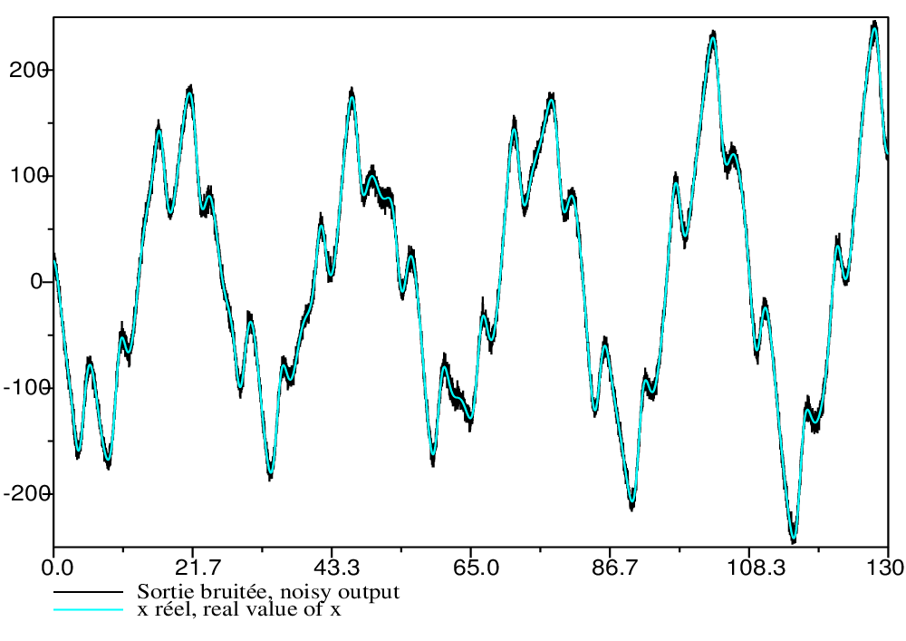
On a pris solution de l’équation , où , avec les conditions initiales et . On a choisi un bruit gaussien avec un écart type de . La sortie est échantillonnée à Hz. On a pris , , si et sinon. Les courbes de la figure 1 résument les résultats obtenus pour et .


On voit qu’après une phase de convergence, l’approximation obtenue est excellente. La précision de l’évaluation des coefficients est naturellement moins bonne quand commence à varier. Toutefois, les évaluations de et demeurent assez précises.
3 Identification avec retards
On considère maintenant un système à retard écrit sous la forme , avec . Soit une fonction telle que , pour avec . On pose . En intégrant par parties, on déduit de l’équation du système
On désignera par cette équation, où le terme a été négligé et chaque puissance remplacée par afin de se ramener à une équation linéaire. Pour et génériques, on résoud par moindres carrés le système , en les inconnues et , où est un ensemble générique d’intervalles d’un cardinal suffisant. On obtient des approximations et des coefficients et et une approximation du retard égale à . La précision du résultat sera d’autant meilleure que le rapport est petit pour chaque couple de .
Une fois obtenue une approximation du retard, on améliore la précision du résultat en résolvant le système , , où , ce qui donnera la nouvelle approximation . On itère le processus.
Pour de meilleurs résultats, on peut également choisir une fonction telle que , par exemple ou .
Exemple 2
Nous avons fait des simulations numériques avec sur l’intervalle pour un système d’ordre . L’équation s’écrit alors et l’on obtient une approximation de égale à à partir d’un système , , où est une estimation préalable du retard.
Les valeurs des coefficients sont les mêmes que celles de l’exemple . On a choisi la commande et un retard . Le bruit est un bruit gaussien et la fréquence d’échantillonnage est de Hz. On a pris pour les couples , . On part de et l’on itère les calculs une cinquantaine de fois (en un temps de l’ordre de quelques secondes sur un Dell Latitude D400), ce qui est suffisant pour atteindre un point fixe à la précision numérique près.
Le tableau ci-dessous, qui donne la moyenne (M.) et l’écart type (É.) de séries de cent estimations des coefficients et du retard réalisées pour des bruits gaussiens d’écarts types croissant, montre que l’on obtient des estimations crédibles, même pour un niveau de bruit notable.
É. bruit M. É. M. É. M. É. M. É. 1 -1,20 0,020 -0,35 0,007 2,00 0,04 4,00 0,015 2 -1,20 0,028 -0,35 0,010 2,00 0,05 4,00 0,023 5 -1,17 0,084 -0.34 0,029 1,94 0,17 3,97 0,065 10 -1,12 0,15 -0,32 0,055 1,84 0,33 3,91 0,132 Tableau 0. Moyenne et écart type des valeurs calculéesTable 0. Mean and standard deviations (É.) of computed values
Nous avons comparé nos résultats avec une méthode souvent utilisée en pratique qui consiste à évaluer les coefficients par une méthode de moindres carrés non linéaire, pour différentes valeurs du retard régulièrement espacées, et à choisir celle pour lesquelles on approche le mieux la sortie. Cette méthode est inapplicable pour l’exemple avec la méthode de moindre carré non linéaire disponible dans scilab, car celle-ci ne converge vers les paramètres que si elle est initialisée avec des valeurs voisines. Toutefois, les moindres carrés non-linéaires permettent d’améliorer la précision de l’évaluation des paramètres et du retard, une fois initialisés avec les résultats fournis par notre méthode. Le tableau ci-dessous fournit les valeurs approchées des écarts types obtenus par notre méthode et après utilisation des moindres carrés (∗), évaluées sur essais, la durée moyenne d’un calcul étant de s.
É. bruit É. É. ∗ É. É. ∗ É. É. ∗ É. É. ∗ É. É. ∗ É. É. ∗ 5 0,1 0,002 0,03 0,0005 0,2 0,002 1 0,4 6 0,5 0,07 0,001 10 0,15 0,005 0,06 0,001 0,35 0,005 1,7 0,6 10 0,9 0,1 0,0015
Tableau 1. Écart type des valeurs calculées
Table 1. Standard deviations of computed values, stared values improved with mean-square
Ce type de calcul suppose, naturellement l’identifiabilité du système. Si la commande est nulle, la sortie constante etc. celui-ci ne sera pas identifiable et il ne le sera que localement pour un comportement périodique. Notons que, nos calculs reposant uniquement sur des résolutions au sens des moindres carrés, il n’y a jamais d’erreurs numériques du type division par . Pour des retard grands, les itérations peuvent diverger et produire une erreur du type invalid index si les intervales d’intégration sortent de la période d’observation du système.
Exemple 3
Cette méthode se généralise au cas de plusieurs retards. Considérons le système . En utilisant sur , on a . En choisissant un nombre suffisant d’intervalles , on peut évaluer par moindres carrés linéaires des approximations de , , et . On en déduit des valeurs de et que l’on peut réinjecter dans les équations pour améliorer la précision.
Les simulations ont été faites avec , , , . L’echantillonage est effectué à avec des bruits gaussiens d’écart-types différents. On a pris et intervalles avec variant par pas de à partir de . Le tableau suivant donne la moyenne et l’écart-type des valeurs calculées (sur 100 essais, chaque calcul durant environ 1,5 s. avec 10 itérations) pour différents niveaux de bruit. Les valeurs de et ne sont naturellement définies que modulo la période de la sortie. La précision du calcul se dégrade si les intervalles n’ont pas une longueur suffisament grande devant et , mais aussi pour un signal périodique si n’est pas assez petit devant la période.
É. du bruit M. É. M. É. M. É. M. É. 0,025 2,69 0,012 1,50 0,006 1,99 0,005 3,99 0,0051 0,05 2,69 0,018 1,49 0,010 1,99 0,010 3,99 0,011 0,1 2,70 0,043 1,50 0,025 1,99 0,01 3,99 0,017 0,2 2,68 0,095 1,48 0,054 1,99 0,039 4,00 0,043
Tableau 2. Moyenne et écart type des valeurs calculées
Table 2. Mean and standard deviations (É.) of computed values
4 Identification en temps réel avec retard lentement variable
On peut également adapter aux systèmes à retard les méthodes d’identification et d’observation en temps réel introduites dans la section 1. On utilise les équations
avec et . Ceci suppose que . On peut s’y ramener quel que soit le retard par un changement d’échelle de temps. L’évaluation du retard est alors . On résoud le système par intégration au moyen d’une méthode de gradient comme décrit section 2. Lorsque , on suppose que les valeurs des estimations sont devenues assez stables (il faut au moins que ne s’annule plus). On pose alors si et sinon. Pour plus de précision, on calcule en posant .
Exemple 4
On utilise les mêmes commande, coefficients, type de bruit et fréquence que pour l’exemple 1. On prend , , et .


Exemple 5
On utilise les mêmes commande, coefficients, type de bruit et fréquence que pour les exemples 1 et 3. On prend , , et . Le retard est initialisé à sa valeur à , afin d’accélérer la convergence.


5 Conclusion
Les méthodes que nous avons introduites permettent un large choix dans leur mise en œuvre. Les quelques essais réalisés montrent qu’elles sont applicables dans des situations réalistes, en particulier avec un niveau de bruit conséquent. Elles peuvent se généraliser aisément, au moins en théorie à des situations plus complexes : retards multiples ou n’intervenant pas uniquemement au niveau de la commande, comme l’illustre l’un de nos exemples.
Leur utilisation suppose la connaissance a priori d’une borne supérieure pour le retard, ce qui est essentiel pour un choix approprié des différents paramètres , , et . En revanche, leur capacité à s’adapter à des coefficients ou à un retard lentement variable nous semble un atout intéressant. Les fichiers utilisés pour les simulations sont disponibles via l’url [13].
Références
- [1] Belkoura (L.), Richard (J.-P.), Fliess (M.) On-line identification of systems with delayed inputs , MTNS’06, 16th Conf. Mathematical Theory of Networks & Systems, 2006.
- [2] Diop (S.), Kolmanovsky (I.), Moraal (P.) et van Nieuwstadt (M.) Preserving stability/performance when facing an unknown time delay , Control Engineering Practice, 9 1319-1325, 2001.
- [3] Fliess (M.), Mounier (H.), On a class of delay systems often arising in practice , Kybernetika, 27, 295-308, 2000.
- [4] Fliess (M.) et Sira-Ramìrez (H.), An algebbraic framework for linear identification , ESAIM Contr. Optim. Cal. Variat., vol. 9, 151–168, 2003.
- [5] Fliess (M.) et Sira-Ramìrez (H.), Reconstructeurs d’état , C.R. Acad. Sci. Paris, 338 (2004), no. 1, 91–96.
- [6] Kolmanovskii (V. B.) et Myshkis (A.), Introduction to the theory and application of functionnal differential equations, Dorctecht, Kluwer Academy, 1999.
- [7] Mahji (S.) Atherton (D. P.), A novel identification method for time delay processes , ECC’99 (Fifth European Control Conference), Karlsruhe, Allemangne, 1999.
- [8] Orlov (Y.) Belkoura (L.) Richard (J. P.) et Dambrine (M.) On-line parameter identification of linear time-delay systems , Proceedings of the 41st IEEE Conference on Decision and Control, Las vegas, Nevada, USA, décembre 2002.
- [9] Richard (J.P.) Time-delay systems : an overview of some recent advances and open problems Automatica, 39, 10, 1667–1694, Octobre 2003.
- [10] Tan (K. K.) Wang (Q. K.) et Lee (T. II.), Finite spectrum assignment control of unstable time delay processes with relay tuning , Industrial Engineering and Chemical Research, 37 (4), 1351–1357, 1998.
- [11] Tuch (J.) Feuer (A.) et Palmor (Z.J.), Time delay estimation in continuous linear time-invariant systems , IEEE Transactions on Automatic Control 39, 823–827.
- [12] Verduyn-Lunel (S. M.), Identification problems in functional differential equations , 36th IEEE CDC’99 (Conference on Decision and Control), San Diego CA, décembre 1997, 4409–4413.
- [13] http://www.lix.polytechnique.fr/~ ollivier/