M/M/$\infty$ queues in semi-Markovian random environmentThanks: Part of this research took place while the author was still post-doc at EURANDOM, Eindhoven, The Netherlands.

The M/M/$\infty$ queue is one of the simplest model in queueing theory. This is due to the joint situation to have a memory-less arrival process and an infinite set of servers that allows customers to behave independently from each other. This suddenly stops to be true after introducing some correlation between customers. In this paper we achieve that by introducing an independent random environment that modulates the system parameters, i.e. the arrival rate and the server speeds. Queues with variable service and arrival speeds arise naturally in practice and therefore many classical works can be found. Most of the results deal with the single server queue, see for example Takine 2005, Ozawa 2004, Sengupta 1990 and references therein. Neuts 1981 analyzed the M/M/1 queue as well as the M/M/C queue in random environment by using the matrix-geometric approach while Takine and Sengupta 1997 looked at the infinite server queue when only the arrival process was subject to a Markovian modulation. The infinite server queue in random environment has then been studied by Keilson and Servi 1993, Baykal-Gursoy and Xiao 2004 and D’Auria 2007 in the special case when the random environment is Markovian and has only two states.

In O’Cinneide and Purdue 1986 the authors looked at the case when the environment is given by a finite state Markov process and for this case they showed how to compute the factorial moments for the number of customers in the system in steady state. Here we extend their analysis to the case of a semi-Markovian random environment.

This extension is interesting as it makes the model more attractive for application purposes. Indeed, despite its simplicity, the M/M/$\infty$ system is often used to model pure delay systems, such as highways, satellite links or long communication cables, or to approximate the behavior of multi server systems. When these kinds of systems are subject to external influences, such as day time changing rates, it is then helpful to look at extended models, such as the one proposed in this work, in order to analyze or predict their behaviors.

The methodology we use follows the technique developed in D’Auria 2007. It consists on representing the stationary and isolate M/G/$\infty$ system as a Poisson process on $\mathbb{R}^{2}$ and by computing the number of customers in the system by measuring a deterministic set according to the point process measure (see also Resnick 1987 and D’Auria and Resnick 2006). In this context the random environment can be expressed as a random modulation of the set and in the special case of exponential distributed service times its measure can be derived by solving a system of stochastic equations, see relation (4.5) below. We use this relation to compute the factorial moments for the number of customers in the system at steady state.

To start, we define the random environment $\{\Gamma(u),u\in\mathbb{R}\}$ as a semi-Markov chain with values in the finite state space $E=\{1,\ldots,{K}\}$. We assume that the sojourn time in the state $k\in E$, denoted as $T_{k}$, is an independent positive random variable whose distribution function has Laplace transform denoted by $\tau_{k}(s):=\mathbb{E}[e^{-sT_{k}}]$. In the following we show that the Laplace transform is the only information we need to compute the moments. When the sojourn time in state $k\in E$ expires, the environment jumps to state $j\in E$ with probability $p_{kj}$. Denoting by ${\bf P}:=\{p_{kj}\}_{k,j\in E}$ the routing matrix that we assume irreducible and with no loss of generality with $p_{kk}=0$, we can define the reverse routing matrix

where ${\bf P}^{\dagger}$ denotes the transpose of the matrix ${\bf P}$, ${\bf\Pi}:=\text{\bf diag}(\vec{\pi})$ and $\vec{\pi}$ is the stationary distribution of the Markov chain generated by ${\bf P}$ (see Brémaud 1999, §6.1).

We assume that when the environment is in state $k\in E$ customers arrive according to a Poisson rate $\lambda_{k}\geq 0$. Each of them brings an independent request of service, $\sigma$, that is exponentially distributed with rate $\mu$. All servers work at constant speed $\beta_{k}=\mu_{k}/\mu\leq 1$. To avoid trivial cases we assume that $\mu,\beta,\lambda>0$ where $\lambda:=\max_{k\in E}\lambda_{k}$ and $\beta:=\max_{k\in E}\beta_{k}$.

By the results in D’Auria 2007 the system is stable and we are allowed to study its stationary regime.

We then look at the system at time $0$ and we count the number of customers still in the system. We order them according to their arrival times $\{u_{h}\}_{h\in\mathbb{Z}}$ with $u_{h}<u_{h+1}$ and $u_{-1}<0\leq u_{0}$, and we denote by $G(\sigma):=1-e^{-\mu\sigma}$, $\sigma>0$, the common exponential distribution function of the $\{\sigma_{h}\}_{h\in\mathbb{Z}}$.

The $h$-th customer, $h<0$, will be in the system at time $0$ iff its service time, $\sigma_{h}$, is bigger than the work done by the server it has occupied during the time interval $[u_{h},0)$. We denote this quantity by $F_{\Gamma}(u_{h})$ and, as the subscript shows, it is a random quantity that depends on the random environment $\Gamma$. Its value can be computed in the following way,

Denoting by $N$ the number of customers in stationary regime we have that it is given by

where $1\{\cdot\}$ is the indicator function of the set $\{\cdot\}$. It is helpful to rewrite the numerable collection of indicator functions appearing in expression (2.3) in the following equivalent way

where $\delta_{(u,\sigma)}$ denotes a Dirac delta measure with center $(u,\sigma)\in\mathbb{R}\times\mathbb{R}^{+}$ and the set $A_{\Gamma}\subset\mathbb{R}^{-}\times\mathbb{R}^{+}$ is given by

This alternative formulation allows the decoupling of the sequence $\{(u_{h},\sigma_{h})\}_{h\in\mathbb{Z}}$ and the function $F_{\Gamma}(u)$ both depending on the realization of the environment $\Gamma$ in the computation of the quantity $N$. Indeed we can express the stationary number of customers in the system in the following way

where

is a point process which locates one Dirac delta measure at each arrival point $\{(u_{h},\sigma_{h})\}_{h\in\mathbb{Z}}$. For the theoretical background and definition of point processes see Daley and Vere-Jones 1988 or Resnick 1987. The subscript $\Gamma$ stays to denote that ${\mathcal{N}_{\Gamma}}$ depends on the random environment by the sequence of arrival times $\{u_{h}\}_{h\in\mathbb{Z}}$. Indeed given a realization $\gamma$ of the process $\Gamma$, the sequence $(\{u_{h}\}_{h\in\mathbb{Z}}|\Gamma=\gamma)$ belongs to an inhomogeneous Poisson process with intensity rate $\lambda_{\gamma(u)}$, $u\in\mathbb{R}$. By Proposition 3.8 in Resnick 1987 it follows that ${\mathcal{N}_{\Gamma}}|\Gamma=\gamma$ is still a Poisson process, now on $\mathbb{R}\times\mathbb{R}^{+}$, with intensity measure

Finally ${\mathcal{N}_{\Gamma}}$ is a doubly stochastic Poisson process or, more briefly, a Cox process (see Daley and Vere-Jones 1988, §8.5), i.e. a Poisson process whose intensity measure is itself random and given by

It is well know that the fidi distributions of a Cox process are of mixed Poisson type (see Daley and Vere-Jones 1988, Corollary 8.5.II), or equivalently that for any set $A\subset\mathbb{R}\times\mathbb{R}^{+}$

is a Poisson random variable whose parameter is itself random with value $|A|_{\Gamma}=\mathbb{E}[{\mathcal{N}_{\Gamma}}(A)|\Gamma]$. $|A|_{\Gamma}$ can be geometrically interpreted as the measure of the set $A$ according to the measure $\lambda_{\Gamma}(\cdot)$, i.e. $|A|_{\Gamma}=\lambda_{\Gamma}(A)$.

From relations (2.5) and (2.8) we finally get that

a mixed Poisson random variable with random parameter $|A_{\Gamma}|_{\Gamma}=\lambda_{\Gamma}(A_{\Gamma})$.

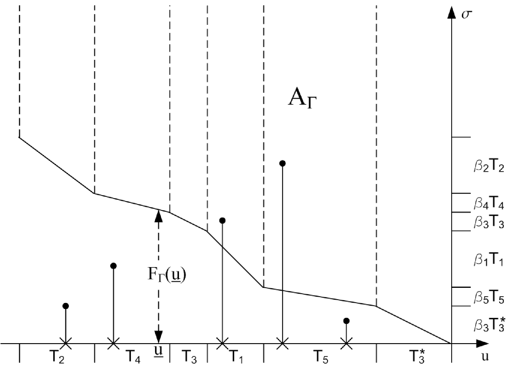
Figure 1 shows an example of realization where the random environment has $K=5$ states: the dots are the centers of the Dirac deltas of the point process ${\mathcal{N}_{\Gamma}}$, while the piecewise linear function $F_{\Gamma}(u)$ denotes the lower bound of the set of integration $A_{\Gamma}$. The customers present in the system at time $0$ are then the ones whose dots fall in the set $A_{\Gamma}$; in the shown example $N=2$.

Before beginning to compute the factorial moments of the random variable $N$, it is worthwhile to review some basic results about the different kinds of moments and their relations with the various generating functions. A good reference about the following relations especially in connection with point processes is Daley and Vere-Jones 1988, Chapter 5.

Given a random variable $X$, we denote by $\psi_{X}(s):=\mathbb{E}[e^{sX}]$ its moment generating function and by $\phi_{X}(z):=\mathbb{E}[z^{X}]$ its probability generating function.

The factorial moment of order $i$ of $X$, $f_{X}^{(i)}$ is defined as

where $p_{n}=\Pr\{X=n\}$ and $n^{\underline{i}}:=n(n-1)\cdots(n-i+1)$ is the falling factorial. It can be directly computed by the $i$-th derivative of the probability generating function, i.e. $f_{X}^{(i)}=\lim_{z\to 1}\phi_{X}^{(i)}(z)$. Knowing the factorial moments of $X$ it is then easy to compute its moments, in the sequel called raw moments to distinguish them from the factorial ones. Indeed, by taking the expectations on both sides of the following known equivalence (Abramowitz and Stegun 1964)

where $\mathfrak{S}_{n}^{(i)}$ is a Stirling Number of the Second Kind, we obtain the following relation between the $n$-th moment of $X$, $m_{X}^{(n)}:=\mathbb{E}\left[X^{n}\right]$ with $m_{X}^{(0)}:=1$, and the factorial moments of order $i\leq n$,

The reverse relation is obtained by using the Stirling Numbers of the First Kind, $\mathfrak{s}_{i}^{(n)}$ (Abramowitz and Stegun 1964, see), that satisfy the following known relation

so that, taking the expectations of both sides, finally we get

It is interesting to notice that relation (3.1) comes directly from using the fact that $\psi_{X}(s)=\phi_{X}(e^{s})$ and that $m_{X}^{(n)}=\lim_{s\to 0}\psi_{X}^{(n)}(s)$. Indeed,

where in the last equation we used Faá di Bruno’s formula for the expansion of derivatives of order $n$ for composition of functions (Abramowitz and Stegun 1964, see) and the fact that $\lim_{s\to 0}\frac{d^{n}}{ds^{n}}e^{s}=1$.

A random variable $X$ is called mixed Poisson when there exists anon-negative random variable $Y$ such that $X\stackrel{{\scriptstyle\rm d}}{{=}}\text{Po}(Y)$, or equivalently $\left(X|Y=y\right)\stackrel{{\scriptstyle\rm d}}{{=}}\text{Po}(y)$, where the operator $\stackrel{{\scriptstyle\rm d}}{{=}}$ denotes equality in distribution. In the case $X$ were a mixed Poisson random variable we would have that

so that taking the derivatives of order $n$, we get

or, in other words, that the factorial moments of $X$ are directly the raw moments of $Y$,

and the latter often are easier to compute.

This is exactly what happens in our case where, as shown by relation (2.9), $N$ is a mixed Poisson and that is why we are interested into its factorial moments rather then directly its raw moments. Indeed we have that the following relation holds

and our task reduces to the computation of the raw moments of the measure of the random set $A_{\Gamma}$.

In this section we compute the raw moments of the measure of the set $A_{\Gamma}$, defined in (2.4), when measured by the random intensity measure $\lambda_{\Gamma}$, defined in (2.7). We use a fixed point technique and to this aim we look at a modified environment process, $\Gamma_{0}$, that is the Palm version of the process $\Gamma$, i.e. we assume that at time $0$ it has a transition. We denote by $k\in E$ the last state it has assumed before $0$, i.e. $k:=\Gamma_{0}(0^{-})$, and by $T_{k}$ its corresponding sojourn time. While, as depicted in Figure 1, for the process $\Gamma$ the sojourn time in the last state before $0$ would be given by a residual sojourn time, for the process $\Gamma_{0}$ it is distributed as any other sojourn time corresponding to the same state. We define by $A_{0k}:=(A_{\Gamma_{0}}|\Gamma_{0}(0^{-})=k)$, $k\in E$, the set $A_{\Gamma_{0}}$ conditioned to the event that the last state occupied by the environment before $0$ is the state $k$, and we call ${|A_{0k}|}$ its measure, i.e. ${|A_{0k}|}:=(\lambda_{\Gamma_{0}}(A_{\Gamma_{0}})|\Gamma_{0}(0^{-})=k)$.

Figure 2 shows an example of the set $A_{0k}$ when $k=3$, together with its decomposition in the set $C_{0k}$ and the set $\mathcal{T}_{T_{3},\beta_{3}T_{3}}A_{05}$. To this we have defined by $C_{0k}$ the restriction of the set $A_{0k}$ up the last transition of the process $\Gamma_{0}$ before time $0$, i.e.

and by $\mathcal{T}_{s,t}A$ the $(-s,t)$-translated version of the set $A$, i.e.

We denote by $j\in E$ the state of the environment before the last transition before time $0$, i.e. $j:=\Gamma_{0}(-T_{k}^{-})$, so that, $-T_{k}$ being a regeneration point for the process $\Gamma_{0}$, we have the independence of the sets $C_{0k}$ and $\mathcal{T}_{T_{k},\beta_{k}T_{k}}A_{0j}$ conditioned to the values of the states before and after the transitions, i.e. $j$ and $k$. $\beta_{k}T_{k}=F_{\Gamma_{0}}(-T_{k})$ is the exact amount of work the non-empty servers have done during the time interval $[-T_{k},0)$ being in state $k$.

By noticing that the set $\mathcal{T}_{T_{k},\beta_{k}T_{k}}A_{0j}$ has measure equal in distribution to ${|\mathcal{T}_{0,\beta_{k}T_{k}}A_{0j}|}:=(\lambda_{\Gamma_{0}}(\mathcal{T}_{0,\beta_{k}T_{k}}A_{0j})|\Gamma_{0}(0^{-})=j)$, we can write down the following set of stochastic equations

where the indicator function $1\{k\leftarrow j\}$ selects the backward state transition of the environment from the state $k$ to the state $j$; this would happen, according to definition (2.1), with probability $q_{kj}$.

Thanks to the fact that along the vertical axis the measure function is given by $G$ that is exponential we have that the following result holds:

By using Lemma 4.1, equation (4.3) simplifies in the following

that is the starting point to prove the following main result:

It is remarkable that it is possible to express equation (4.6) in terms of the forward transition chain ${\bf P}$. The result is contained in the following corollary whose proof comes from simple matrix computations.

Given the raw moments of the ${|A_{\Gamma_{0}}|}$, we can successively compute the moments of the measures of the sets $A_{k}:=(A_{\Gamma}|\Gamma(0)=k)$, $k\in E$. Following previous definitions we define $m^{(n)}_{k}:=m^{(n)}_{{|A_{k}|}}$. Similarly to equation (4.3) we have the following equation

with ${|C^{*}_{k}|}=\rho_{k}(1-e^{-\mu_{k}T^{*}_{k}})$. $T^{*}_{k}$ refers to a residual sojourn time of the environment in state $k\in E$. We define by $\tau^{*}_{k}(s)$ the Laplace transform of the distribution function of $T^{*}_{k}$ and it is related to the one of $T_{k}$, $\tau_{k}(s)$, by the relation $\tau^{*}_{k}(s)=\bar{\tau}_{k}(1-\tau_{k}(s))/s$, with $\bar{\tau}_{k}:=\mathbb{E}[T_{k}]^{-1}$. For the vector of raw moments $\vec{m}^{(n)}$ the following theorem holds.

In order to check our results we compare equation (4.15) for the exponential case with results in O’Cinneide and Purdue 1986 here repeated in formula (4.22). For this case since $T^{*}_{k}\stackrel{{\scriptstyle\rm d}}{{=}}T_{k}$, we have that $\vec{m}^{(n)}=\vec{m}_{0}^{(n)}$.

Formulas (4.7) and (4.18) show that generally to find the $n$-th moment of the random number of users in the system involves in a complex way the knowledge of all previous moments. Reversely the exponential case, that was already solved in O’Cinneide and Purdue 1986, is easier as the $n$-th vector of moments is related only by a factor to the $(n-1)$-th one. That was anyway hidden in a non-trivial way in formula (4.7) so that there could be some other special cases where an easier expression holds.

In this section we have a look to the case when the environment has only two stages, i.e. ${K}=2$.

This is a very special case and when the sojourn times are all assumed exponentially distributed, it is known how to compute the complete distribution of the number of customers in the system at steady state (see Keilson and Servi 1993, Baykal-Gursoy and Xiao 2004 and D’Auria 2007).

We give for this case an explicit formula to calculate the factorial moments in terms of the Laplace transform of the sojourn time in state $1$, when the sojourn time in state $2$ is exponentially distributed.

By rewriting in more explicit form equation (4.9) for the case ${K}=2$ we get

We define $\tilde{m}_{0k}^{(n)}:=\mathbb{E}[({|A_{0k}|}-\rho_{1})^{n}]$ and take the mean of the $n$-powers of expression (5.1) so getting

By adding and subtracting $\rho_{1}$ to both sides of equation (5.2) we get

with $\rho_{*}=\rho_{2}-\rho_{1}$. Then using equation (5.1) we obtain a recursive equation involving only ${|A_{02}|}-\rho_{1}$,

Taking the $n$-th power and then the expectation of both sides we get

that, taking into account equation (5.3), can be rearranged to get the following

References

- Abramowitz and Stegun (1964) M. Abramowitz and I. A. Stegun (1964): Handbook of Mathematical Functions with Formulas, Graphs, and Mathematical Tables. Dover, New York.
- Baykal-Gursoy and Xiao (2004) M. Baykal-Gursoy and W. Xiao (2004): Stochastic Decomposition in Queues with Markov-Modulated Service Rates. Queueing Syst. 48:75–88.
- Brémaud (1999) P. Brémaud (1999): Markov Chains. Springer, New York.
- Daley and Vere-Jones (1988) D. J. Daley and D. Vere-Jones (1988): An Introduction to the Theory of Point Processes. Springer Series in Statistics. Springer-Verlag, New York, 1st edition.
- D’Auria (2007) B. D’Auria (2007): Stochastic decomposition of the queue in a random environment. Oper. Res. Lett. 35:805–812.
- D’Auria and Resnick (2006) B. D’Auria and S. Resnick (2006): Data Network Models of Burstiness. Adv. in Appl. Probab. 38:373–404.
- Keilson and Servi (1993) J. Keilson and L. Servi (1993): The matrix system: Retrials models and Markov modulated sources. Adv. in Appl. Probab. 25:453–471.
- Neuts (1981) M. Neuts (1981): Matrix–Geometric Solutions in Stochastic Models: An Algorithmic Approach.. Johns Hopkins University Press.
- O’Cinneide and Purdue (1986) C. O’Cinneide and P. Purdue (1986): The queue in a random environment. J. Appl. Probab. 23:175–184.
- Ozawa (2004) T. Ozawa (2004): Analysis of Queues with Markovian Service Processes. Stochastic Models 20:391–413.
- Resnick (1987) S. Resnick (1987): Extreme Values, Regular Variation and Point Processes. Springer-Verlag, New York.
- Seneta (1981) E. Seneta (1981): Non-Negative Matrices and Markov Chains. Springer Series in Statistics. Springer Verlag, New York, 2nd edition.
- Sengupta (1990) B. Sengupta (1990): A Queue with Service Interruptions in an Alternating Random Environment. Operations Research 38:308–318.
- Takine (2005) T. Takine (2005): Single-Server Queues with Markov-Modulated Arrivals and Service Speed. Queueing Syst. Theory Appl. 49:7–22.
- Takine and Sengupta (1997) T. Takine and B. Sengupta (1997): A Single Server Queue with Service Interruptions. Queueing Syst. 26:285–300.