A Recipe for Symbolic Geometric Computing: Long Geometric Product, BREEFS and Clifford Factorization

Using geometric invariants in symbolic geometric computing has been an active research subject in symbolic and algebraic computation. Apart from the benefit of better geometric interpretability when compared with coordinates [13], geometric invariants have a salient feature of reducing the size of symbolic manipulation. This is particularly valuable because a major difficulty in symbolic computing is middle expression swell.

In projective incidence geometry, the proofs of many theorems by the method of biquadratic final polynomials [3] can be so elegant that only bracket binomials occur in the whole procedure. The area method [2] also shares this feature in its ratio-formed proofs of many theorems, i.e., the numerators and denominators are monomials of areas. The advantages of both methods are assimilated into the Cayley expansion theory developed in [11], by which this feature of projective incidence geometry is extended to projective conic geometry.

In Euclidean geometry, with the introduction of inner products, syzygies among basic invariants become much more complicated. Using distances for geometric theorem proving was proposed in [4], and further developed in [12] by including the inner products of extensors. In [8] the covariant algebra of Euclidean geometry, the so-called conformal geometric algebra (CGA), and its invariant subalgebra, the so-called null bracket algebra, was shown to provide a nice algebraic setting for Euclidean geometric theorem proving. Unfortunately, except for some sporadic special cases, none of these methods has ever shown any binomial feature. As a benchmark problem, Miquel’s 5-circle theorem [2], whose analytic proof is straightforward but very difficult symbolic computing, was found a proof of 14 terms in 2001 [9]. The proof was full of pairwise term reductions based on complicated syzygies of advanced invariants.

Under such background it comes as appalling as can be an observation that symbolic computing and theorem proving in Euclidean geometry have a “monomial” feature, or more generally, a term preservation feature in the language of NBA, if the recipe in this paper is used.

By the time this paper is being written, $70+$ Euclidean geometric theorems in [1] have been tested, and $40+$ have the term preservation feature. In particular, $30+$ theorems have their conclusions represented by monomials in NBA, and are kept as monomials till the end of the proof. Concrete examples include all the examples published in [8]. Using the method in that paper only one example preserves its number of terms in the proof. Using our recipe in this paper ALL examples preserve their number of terms, thus it is impossible to find any analytic proof that is more elegant.

By preserving the number of terms the computing burden is transmitted from addition to noncommutative multiplication. One may shake head as to any possible simplification by algebraic manipulation of multiplication in place of addition. Well, in an invariant symbolic system there are syzygies among basic elements. In manipulating such elements, multiplication preserves geometry while addition breaks it up. Symmetries in multiplication provide the most economical way of avoiding or employing syzygies. It is easy to change multiplication to addition: just recall how coordinates are introduced. Generally it is very difficult to change addition to multiplication: just recall Cayley factorization [14] in projective geometry.

Our recipe for symbolic computing in Euclidean geometry is: (1) employ multiplication, or more accurately, the geometric product in Geometric Algebra, from the representation of geometric objects on, (2) preserve the multiplication through subsequent algebraic manipulation using the principle “BREEFS” [11], and (3) replace addition by multiplication using Clifford factorization – the Euclidean version of Cayley factorization. In (1) we need to invent two new devices for the representation by multiplication, called nullifying operator and reduced meet product. In (2) we need to adapt the previous global invariant bracket-oriented principle to a shift invariant neighborhood principle. In (3) we need a device to explore rational Clifford expansions systematically – pseudodivision in NBA. These novelties will be introduced in Sections 4 and 5, with various illustrations.

Geometric Algebra [5] is a version of Clifford algebra favoring the universal usage of its multiplication, the geometric product, instead of addition. Hestenes’ vision of Geometric Algebra in place of the more commonly used Clifford algebra in matrix or hypercomplex numbers form, is fully justified by our theorem proving practice: replacing addition by multiplication and prolonging the multiplication (“long geometric product”), are the simplest means of avoiding syzygies because the geometric product already incorporates various syzygies of inner products and determinants into its structural symmetry.

The Geometric Algebras developed for the conformal model of Euclidean geometry, CGA [6] and NBA [7], will be introduced in Section 2 from the implementation point of view. The geometry of long geometric product in NBA will be explained in Section 3. In the end of this paper, a 3-termed analytic proof will be provided for the benchmark problem, Miquel’s 5-circle theorem.

In [6], [7], [8] there have been detailed introductions of CGA and NBA. In this paper we concentrate on the case of 2D geometry only. We always use a boldfaced number or letter to denote a vector.

In 4D Minkowski space we fix a null vector ${\bf e}$. A null vector is a nonzero vector whose inner product with itself is zero. We call ${\bf e}$ the point at infinity of the Euclidean plane. Any null vector linear independent of ${\bf e}$ is a point in the plane. Two null vectors represent the same point if and only if they differ only by scale. This representation of the Euclidean plane is conformal but not isometric. To obtain an isometric model we only need to fix the inner product of any point with the point at infinity, e.g. to $-1$, as any two linear independent null vectors have nonzero inner product.

To describe and analyze Euclidean geometry with the conformal model we need a suitable algebraic language. The symbolic version of Clifford algebra in [5] is an ideal tool in that it prefers the usage of multiplication to addition. The multiplication, called geometric product, conglomerates all geometric relations within itself and is geometrically meaningful. The other two versions, the matrix version and the hypercomplex numbers version, emphasize the linear nature of the algebra, i.e., care more for addition than for multiplication. In symbolic form, more addition leads to more algebra, and more multiplication preserves more geometry. This justifies the gist “geometric” in Hestenes’ Geometric Algebra.

Geometric Algebra is the unique algebra generated from an $n$D inner product space by an associative product, called geometric product, satisfying the generating relation that the geometric product of any vector with itself is the inner product. The geometric product is always denoted by juxtaposition.

Geometric Algebra is graded, the grade ranges from 0 to $n$. For an element $A$ in this algebra, the $i$-graded part is denoted by $\langle A\rangle_{i}$. When $i=0$ and 1 it is the scalar and vector part respectively. Elements of grade $i$ form a subspace of dimension $C_{n}^{i}$. In particular when $i=n$, the $n$-graded subspace is 1D. Fix a nonzero element $I_{n}$ in this space, then for any other $n$-graded element $A_{n}$, the coordinate of $A_{n}$ with respect to the basis $I_{n}$ is the bracket of $A_{n}$:

The geometric product of an element $A$ with $I_{n}^{-1}$ is called the dual of $A$: $A^{\sim}=AI_{n}^{-1}$. In particular $A_{n}^{\sim}=[A_{n}]$.

The geometric product of two vectors is composed of two parts, the 0-graded part and the 2-graded part. They are respectively the inner product and outer product, denoted by dot and wedge. The outer product is just the exterior product in Grassmann’s exterior algebra.

For three vectors,

Conformal geometric algebra (CGA) [6] is the Geometric Algebra established upon the conformal model. In CGA for 2D geometry, we can pick out two scalar-valued functions generated by a sequence of $2k$ null vectors ${\bf 1},{\bf 2},\cdots$, ${\bf 2k}$: the 0-graded part

called the angular bracket, and the bracket of the 4-graded part for $k>1$:

called the square bracket. The two kinds of brackets generate a ring called null bracket algebra (NBA) [7], [8].

NBA should be implemented by realizing the following basic properties:

(1) Multilinearity of geometric product, multilinearity and (anti-)symmetry of inner product and outer product, (2.2) and (2.3) from left to right.

(2) Null symmetry: for null vector ${\bf 1}$,

(3) Shift and reversion symmetry: for vectors $\bf 1,2,\cdots,k$,

(4) Dual symmetry: for element $A$ and $r$-graded element $B_{r}$,

(5) Points ${\bf 1},{\bf 2},{\bf 3}$ are collinear: $[{\bf e}{\bf 1}{\bf 2}{\bf 3}]=0;$ points ${\bf 1},{\bf 2},{\bf 3},{\bf 4}$ are cocircular: $[{\bf 1}{\bf 2}{\bf 3}{\bf 4}]=0.$ Lines ${\bf 1}{\bf 2},{\bf 1}^{\prime}{\bf 2}^{\prime}$ are parallel:
$[{\bf e}{\bf 1}{\bf 2}{\bf e}{\bf 1}^{\prime}{\bf 2}^{\prime}]=0$; they are perpendicular: $\langle{\bf e}{\bf 1}{\bf 2}{\bf e}{\bf 1}^{\prime}{\bf 2}^{\prime}\rangle=0$.

(6) Contraction by Grassmann-Plücker syzygy: for vectors ${\bf 1},{\bf 2},{\bf 3},{\bf 4},{\bf 5},{\bf 1}^{\prime},{\bf 2}^{\prime},{\bf 3}^{\prime}$,

(7) Contraction by inner-product bracket syzygy: for vectors ${\bf 1},{\bf 2}$, ${\bf 3},{\bf 4},{\bf 5},{\bf 1}^{\prime}$,

(8) Null expansion: for null vector ${\bf 1}$,

(9) Trigonometric quartet expansion: for null vector ${\bf 1}$,

(10) Trigonometric sextet expansion: for null vector ${\bf 1}$,

(11) Rational sextet expansion: for null vectors ${\bf 2},{\bf 3},{\bf 5},{\bf 6}$,

(12) Rational octet expansion: for null vectors ${\bf 1},{\bf 2},{\bf 3},{\bf 5}$,

(13) Reverse of the expansions from (2.12) to (2.15): from right to left. They are basic Clifford factorizations.

The derivation of the properties is easy. In Section 3, (2.12) and (2.13) are discussed, in Section 5, (2.14) and (2.15) are analyzed.

Prolonging the length of elements in inner products and brackets (i.e., determinants) is not only a device of simplifying symbolic computing, but an indispensable means of representing basic geometric relations. We take a look at a planar angle and its algebraic representation.

An oriented angle is just a 2D rotation. $\angle{\bf 1}{\bf 2}{\bf 3}$ can be represented by three points: the vertex ${\bf 2}$, a point ${\bf 1}$ on the initial ray, and a point ${\bf 3}$ on the terminal ray without requiring that ${\bf 1},{\bf 3}$ be equidistant from ${\bf 2}$. Without resorting to inequalities, any rational description of angle $\angle{\bf 1}{\bf 2}{\bf 3}$ by points ${\bf 1},{\bf 2},{\bf 3}$ is accurate only up to $k\pi$. The equivalent classes of oriented planar angles modulo $\pi$ are called full angles [2].

Let $\angle{\bf 1}{\bf 2}{\bf 3},\angle{\bf 1}^{\prime}{\bf 2}^{\prime}{\bf 3}^{\prime}$ be two full angles. They are equal if and only if $\tan\angle{\bf 1}{\bf 2}{\bf 3}=\tan\angle{\bf 1}^{\prime}{\bf 2}^{\prime}{\bf 3}^{\prime}$. In the conformal model, the ratio of $[{\bf e}{\bf 1}{\bf 2}{\bf 3}]$ to $\langle{\bf e}{\bf 1}{\bf 2}{\bf 3}\rangle$ is exactly $\tan\angle{\bf 1}{\bf 2}{\bf 3}$. So $\angle{\bf 1}{\bf 2}{\bf 3}=\angle{\bf 1}^{\prime}{\bf 2}^{\prime}{\bf 3}^{\prime}$ if and only if

i.e.,

Essentially, geometric product ${\bf e}{\bf 1}{\bf 2}{\bf 3}$ represents full angle $\angle{\bf 1}{\bf 2}{\bf 3}$, its sine and cosine are respectively the square and angular brackets, its reverse angle is ${\bf e}{\bf 3}{\bf 2}{\bf 1}$. ${\bf e}{\bf 1}{\bf 2}{\bf e}{\bf 3}{\bf 4}$ represents full angle $\angle(\overrightarrow{\bf 12},\overrightarrow{\bf 34})$. The sum of full angles ${\bf e}{\bf 1}{\bf 2}{\bf 3},{\bf e}{\bf 1}^{\prime}{\bf 2}^{\prime}{\bf 3}^{\prime}$ is their concatenation ${\bf e}{\bf 1}{\bf 2}{\bf 3}{\bf e}{\bf 1}^{\prime}{\bf 2}^{\prime}{\bf 3}^{\prime}$. These explain (2.12) and (2.13) as expansions of the sines and cosines of angle sums.

Using null expansion (2.11) and trigonometric expansions (2.12) and (2.13), we easily obtain trigonometric explanations of all square and angular brackets. For example if ${\bf e}$ does not occur in the following vectors, then

and for the general case,

Here $d_{{\bf 1}{\bf 2}}$ is the Euclidean distance between points ${\bf 1},{\bf 2}$; $\overrightarrow{{\bf 1}{\bf 2}{\bf 3}}$ denotes the oriented circle through ${\bf 1},{\bf 2},{\bf 3}$ sequentially, and $\angle(\overrightarrow{{\bf 1}{\bf 2}{\bf 3}},\overrightarrow{{\bf 1}{\bf 3}{\bf 4}})$ is the full angle from the tangent direction of $\overrightarrow{{\bf 1}{\bf 2}{\bf 3}}$ to that of $\overrightarrow{{\bf 1}{\bf 3}{\bf 4}}$ at any point of their intersection.

If ${\bf e}$ occurs then the explanation is only slightly changed. For example,

and the general case follows similarly. The power of long geometric product comes from its intrinsic geometric nature.

Below we present two novel devices in NBA, the nullifying operator and the reduced meet product. They function as the bridge between Grassmann-Cayley algebra and NBA, thus allowing to employ the full power of Cayley expansion theory [11] within Euclidean geometry.

Let ${\bf 1}$ be a null vector in 4D Minkowski space. For vector ${\bf 2}$,

is the nullification of ${\bf 2}$ with respect to ${\bf 1}$. When ${\bf 2}$ is null then $N_{\bf 1}({\bf 2})=({\bf 1}\cdot{\bf 2}){\bf 2}$ represents the same point ${\bf 2}$. When ${\bf 2}$ is not null, then $N_{\bf 1}({\bf 2})$ represents the null vector other than ${\bf 1}$ in the plane spanned by ${\bf 1},{\bf 2}$ if the metric of the plane is Minkowski, or just ${\bf 1}$ if the metric is degenerate.

The reduced meet product of two elements ${\bf 2}\wedge{\bf 3}$ and ${\bf 2}^{\prime}\wedge{\bf 3}^{\prime}$ modulo vector ${\bf 1}$ is

The second equality is modulo ${\bf 1}$, i.e., the two sides differ by $\lambda\,{\bf 1}$ for a scale $\lambda$. This product is a reduced form of the classical meet product of elements ${\bf 1}\wedge{\bf 2}\wedge{\bf 3}$ and ${\bf 1}\wedge{\bf 2}^{\prime}\wedge{\bf 3}^{\prime}$:

Proposition 1. [Null duality] Let ${\bf 1}^{\prime}$ be a null vector, then

Proof. In Geometric Algebra we have the duality relation

so

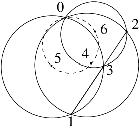
Example 1. [See [8], Example 5] If three circles having a point in common intersect pairwise at three collinear points, their common point are cocircular with their centers.

This is the most difficult example in [8]. We use the same geometric scenario: remove the collinearity constraint from the hypotheses, compute the conclusion expression to see if the removed constraint comes out as a factor.

Same as in [8], during the computing all intermediate factors are saved in a set for later analysis. They are marked with under braces and are removed from subsequent steps.

Free points: $\bf 0,1,2$.
Centers: ${\bf 4}={\rm center}({\bf 0}{\bf 1}{\bf 2}),\ {\bf 5}={\rm center}({\bf 0}{\bf 1}{\bf 3})$, ${\bf 6}={\rm center}({\bf 0}{\bf 2}{\bf 3})$.
Removed hypothesis: $[{\bf e}{\bf 1}{\bf 2}{\bf 3}]=0$.
Conclusion expression: $[{\bf 0456}]$.

The center of circle ${\bf 1}{\bf 2}{\bf 3}$ is

Substitute the expressions of the three circle centers ${\bf 4},{\bf 5},{\bf 6}$ into the conclusion, we get

Explanation of the computing:

Line 1: substitution.
Line 2: change of order by symmetries (2.8) and (2.7).
Line 3: apply (4.22) to the first two pairs of meet products.
Line 4: expand meet products, make null expansion (2.11).
Line 5: apply (2.3). Only one term is generated.
Line 6: change of order between neighboring ${\bf 0}$’s by (2.6).
Line 7: null expansion.

Now consider the most typical geometric construction: the intersection of two circles. Let ${\bf 1}{\bf 2}{\bf 3}$ and ${\bf 1}{\bf 2}^{\prime}{\bf 3}^{\prime}$ be two circles represented by circumpoints. Their point of intersection, denoted by ${\bf 1}{\bf 2}{\bf 3}\cap{\bf 1}{\bf 2}^{\prime}{\bf 3}^{\prime}$, refers to the point of intersection other than ${\bf 1}$, or in the tangent case, tangent point ${\bf 1}$ itself. When ${\bf 1}={\bf e}$ it is the intersection of lines ${\bf 2}{\bf 3},{\bf 2}^{\prime}{\bf 3}^{\prime}$; when ${\bf 2}={\bf e}$ it is the intersection of line ${\bf 1}{\bf 3}$ and circle ${\bf 1}{\bf 2}^{\prime}{\bf 3}^{\prime}$.

In [7] the intersection was expressed as a linear combination of three vectors: either ${\bf 1},{\bf 2},{\bf 3}$, or ${\bf 1},{\bf 2}^{\prime},{\bf 3}^{\prime}$. In this paper we propose the following representation:

It is easily verified that (4.25) equals the expressions in [7].

In (4.25) the reduced meet product has two ways of expansion, either by separating ${\bf 2},{\bf 3}$ as in the first line of (4.20), or by separating ${\bf 2}^{\prime},{\bf 3}^{\prime}$. If we compute the geometric product

then previously we simply expanded the meet products in the same way and multiplied them with ${\bf 1}$. Since the geometric product is associative, not only can we expand the meet products in different ways, but we can freely change the order of the four pairwise geometric products in (4.26). Furthermore, if the intersection has more than one construction, e.g. it is where three lines meet, we can even change the representations by different pairs of lines for each meet product. By prolonging the length of the geometric product, we gain a lot of freedom for the realization of “BREEFS”.

BREEFS – “Bracket-oriented Representation, Elimination and Expansion for Factored and Shortest result”, was first proposed in [11] to control the expression size in bracket algebra. In [8] it was extended to null inner-product bracket algebra, the subalgebra of NBA generated by angular brackets of length 2 and square brackets of length 4. In this section we extend it to long geometric products. The best way to explain this principle is through some working examples.

Example 2. In the plane two circles intersect at points ${\bf 1},{\bf 1}^{\prime}$. Two secant lines through them intersect the circles at points ${\bf 2},{\bf 3}$ and ${\bf 2}^{\prime},{\bf 3}^{\prime}$ respectively. Then ${\bf 2}{\bf 2}^{\prime}//{\bf 3}{\bf 3}^{\prime}$.

In [8] one hypothesis of the theorem was removed and a geometric factorization of the conclusion was obtained. In [10] two hypotheses were removed and a geometric completion was discovered. The computing was 3-termed in [8] and 2-termed in [10]. Both required Clifford factorization, [8] further used circular transform. Below we present a 1-termed computing without Clifford factorization nor transform.

The configuration in Figure 2b is constructed as follows:

Free points: ${\bf 1},{\bf 2},{\bf 3},{\bf 1}^{\prime},{\bf 2}^{\prime}$.
Intersection: ${\bf 3}^{\prime}={\bf 1}^{\prime}{\bf 2}^{\prime}\cap{\bf 1}{\bf 3}{\bf 1}^{\prime}$.
Conclusion expression: $[{\bf e}{\bf 2}{\bf 2}^{\prime}{\bf e}{\bf 3}{\bf 3}^{\prime}]$.

BREEFS in (5.27):

(1) The first meet product has two neighbors in the long geometric product: ${\bf 3}$ and ${\bf 1}^{\prime}$. Expansion by separating ${\bf 1},{\bf 3}$ would simply replace the meet product by ${\bf 1}$. Separating ${\bf e},{\bf 2}^{\prime}$ would produce two terms and a Clifford factorization (2.14) must be used to get a monomial result.

(2) Similarly, the expansion of the second meet product has to separate ${\bf e},{\bf 2}^{\prime}$, as ${\bf e}$ is a neighbor by shift symmetry. The last step uses null symmetry (2.6) and null expansion (2.11):

The result is not what we expected. The two brackets $[{\bf e}{\bf 1}{\bf 2}{\bf 3}]$ and $[{\bf 1}{\bf 2}{\bf 1}^{\prime}{\bf 2}^{\prime}]$ representing the two removed hypotheses are not in the final result. They can be produced by rational expansion (2.14):

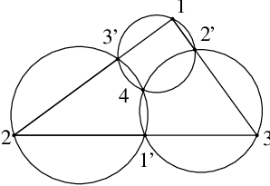
Example 3. [See [8], Example 3] Let $\bf 1^{\prime},2^{\prime},3^{\prime}$ be points on sides $\bf 23,13,12$ of triangle $\bf 123$ respectively. Then circles $\bf 12^{\prime}3^{\prime}$, $\bf 1^{\prime}23^{\prime}$ and $\bf 1^{\prime}2^{\prime}3$ meet at a common point ${\bf 4}$.

In [8] a collinearity constraint was removed in order to explore the dependency of the conclusion upon the constraint. Below we remove all the hypotheses (the three collinearity constraints) to explore the equivalence of the conclusion with the hypotheses.

Conclusion: three circles ${\bf 1}{\bf 2}^{\prime}{\bf 3}^{\prime}$, ${\bf 1}^{\prime}{\bf 2}{\bf 3}^{\prime}$, ${\bf 1}^{\prime}{\bf 2}^{\prime}{\bf 3}$ concur, i.e., the intersection ${\bf 4}={\bf 1}{\bf 2}^{\prime}{\bf 3}^{\prime}\cap{\bf 1}^{\prime}{\bf 2}{\bf 3}^{\prime}$ is on circle ${\bf 1}^{\prime}{\bf 2}^{\prime}{\bf 3}$:

In conclusion expression $[{\bf 1}^{\prime}{\bf 2}^{\prime}{\bf 3}{\bf 4}]$, ${\bf 1}^{\prime},{\bf 2}^{\prime},{\bf 3}$ are antisymmetric. Because ${\bf 3}$ is irrelevant to ${\bf 4}={\bf 1}{\bf 2}^{\prime}{\bf 3}^{\prime}\cap{\bf 1}^{\prime}{\bf 2}{\bf 3}^{\prime}$, only when ${\bf 4}$ is between ${\bf 1}^{\prime},{\bf 2}^{\prime}$ can the BREEFS principle take effect. Then similar to Example 2, neighborhood consideration leads to unique monomial expansions of the meet products.

Discarded hypotheses: three “circles” ${\bf 1}^{\prime}{\bf 2}{\bf 3}$, ${\bf 1}{\bf 2}^{\prime}{\bf 3}$, ${\bf 1}{\bf 2}{\bf 3}^{\prime}$ concur (at “point” ${\bf e}$). This can be represented by the incidence of the intersection ${\bf 1}^{\prime}{\bf 2}{\bf 3}\cap{\bf 1}{\bf 2}^{\prime}{\bf 3}$ and circle ${\bf 1}{\bf 2}{\bf 3}^{\prime}$. Simply by interchanging the primes over the same letters, we get from (5.28) the same effective part of the discarded hypotheses:

(5.29) discloses the intrinsic equivalence between the conclusion and the hypotheses.

Example 4. [Miquel’s 4-circle Theorem] Four circles intersect sequentially at pairs of points $({\bf 1},{\bf 5})$, $({\bf 2},{\bf 7})$, $({\bf 3},{\bf 6})$ and $({\bf 4},{\bf 8})$. If ${\bf 1},{\bf 2},{\bf 3},{\bf 4}$ are cocircular then so are ${\bf 5},{\bf 6},{\bf 7},{\bf 8}$.

This is a typical theorem whose analytic proof using coordinates is difficult although straightforward. In [7] a 5-termed NBA proof was found. Below we present a 1-termed proof.

Free points: $\bf 1,2,3,4,5,6$.
Intersections: ${\bf 7}={\bf 1}{\bf 2}{\bf 5}\cap{\bf 2}{\bf 3}{\bf 6},\ \ \ {\bf 8}={\bf 1}{\bf 4}{\bf 5}\cap{\bf 3}{\bf 4}{\bf 6}.$

Similar to Example 3, neighbors of ${\bf 7},{\bf 8}$ in bracket $[{\bf 5}{\bf 6}{\bf 7}{\bf 8}]$ should be changed to ${\bf 5},{\bf 6}$ to make the best of the BREEFS principle. The rest are two simple null expansions leading to the conclusion $[{\bf 1}{\bf 2}{\bf 3}{\bf 4}]$. If using the original $[{\bf 5}{\bf 6}{\bf 7}{\bf 8}]$, then the two meet products

are neighbors in the long geometric product. They share two pairs of points: $({\bf 1},{\bf 5})$ and $({\bf 3},{\bf 6})$, and should be expanded by separating the same pair. The result is 2-termed, and Clifford factorization (2.14) must be used to return to one term.

Summary of “BREEFS” in NBA:

(1) To get factored and shortest result, choose suitable algebraic representations, do eliminations and expansions in long geometric products according to neighborhood consideration. Immediate neighbors have topmost priority, then next immediate neighbors, and so on. (2) If neighbors of a meet product can be altered, then rearrange neighbors by relevance to the meet product. (3) If an outer product is common to neighboring meet products, expand the meet products by splitting common outer product.

Below we discuss Clifford factorizations (2.14) to (2.15) which are inverse of rational Clifford expansions. They are the most important devices to reduce the number of terms of bracket polynomials. In particular, the first formula of (2.14) is the MOST frequently used Clifford factorization. Its proof is straightforward substitution of the Cramer’s rule of ${\bf 4}$ (or ${\bf 1}$) with respect to basis ${\bf 2},{\bf 3},{\bf 5},{\bf 6}$:

into bracket $[{\bf 1}{\bf 2}{\bf 3}{\bf 4}{\bf 5}{\bf 6}]$ and then null expansion (2.11). All other rational Clifford expansion formulas are easily proved in this way. However, the proof does not provide any explanation as to why from the left to right of (2.14) one should add the factor $[{\bf 2}{\bf 3}{\bf 5}{\bf 6}]$, and why the right side should contain any of the factors on the left.

(2.14) from left to right can be understood from the aspect of pseudodivision. In Example 2, $[{\bf 1}{\bf 2}{\bf 3}{\bf 4}{\bf 5}{\bf 6}]$ in (2.14) needs to be pseudodivided by $[{\bf 3}{\bf 4}{\bf 5}{\bf 6}]$ and $[{\bf 1}{\bf 2}{\bf 3}{\bf 6}]$ to get the quotients. If ${\bf 4}$ is the leading vector variable, then since divisor $[{\bf 3}{\bf 4}{\bf 5}{\bf 6}]$ is linear with respect to ${\bf 4}$, we can substitute the expression of ${\bf 4}$ by ${\bf 3},{\bf 5},{\bf 6}$ into the dividend to get a remainder. Similarly, if ${\bf 1}$ is the leading vector variable and $[{\bf 1}{\bf 2}{\bf 3}{\bf 6}]$ is the divisor, we can substitute the expression of ${\bf 1}$ by ${\bf 2},{\bf 3},{\bf 6}$ into the dividend to get another remainder. The unique common pseudocoefficient for both pseudodivisions is $[{\bf 2}{\bf 3}{\bf 5}{\bf 6}]$. Thus the quotients can be obtained by substituting (5.31) into the dividend.

To understand (2.14) from right to left is much more difficult. However, once a factor say $[{\bf 2}{\bf 3}{\bf 5}{\bf 6}]$ is discovered from the right, e.g., by polynomial factorization in homogeneous coordinates, then the other factor $f$ can be easily fixed. Since $f$ is a multilinear function of its vector variables, a procedure similar to multilinear Cayley factorization [14] leads to the result that $f$ equals $[{\bf 1}{\bf 2}{\bf 3}{\bf 4}{\bf 5}{\bf 6}]$ up to a constant factor.

Example 5. [Miquel’s 5-circle Theorem] Let there be a five star with vertices $\bf 1^{\prime},2^{\prime},3^{\prime},{\bf 4}^{\prime},{\bf 5}^{\prime}$, and armpit points $\bf 1,2,3,4$, ${\bf 5}$. The circumcircles of the five triangular wedges meet sequentially at shoulder points $\bf 1^{\prime\prime},2^{\prime\prime},3^{\prime\prime},4^{\prime\prime},5^{\prime\prime}$ respectively. Then the shoulder points are cocircular.

There is another saying is that this theorem is due to W. K. Clifford, the inventor of Clifford algebra. Its analytic proof is straightforward but complicated symbolic computing. In this section we present a 3-termed beautiful proof with no short of elegance than traditional synthetic one.

We use the same construction of the configuration as in [9]: first the armpit points ${\bf 1},{\bf 2},{\bf 3},{\bf 4},{\bf 5}$ as free points; then the vertices as intersections of lines:

finally the shoulder points as intersections of circles:

By symmetry we only need to prove $[{\bf 1}^{\prime\prime}{\bf 2}^{\prime\prime}{\bf 3}^{\prime\prime}{\bf 4}^{\prime\prime}]=0$.

Consider the expansion of the first meet product. Its immediate neighbors provide no hint. A next immediate neighbor is ${\bf 2}$, suggesting the separation of ${\bf 1}^{\prime},{\bf 2}$. Similarly, for the second meet product, its next immediate neighbor ${\bf 1}$ suggests the expansion by separating ${\bf 1},{\bf 1}^{\prime}$. The two expansions result in three terms from the first two meet products:

Suddenly it appears that the first two meet products are simply removed from (6.32):

Although irrelevant to the proof, It is interesting to note that after eliminating ${\bf 1}^{\prime},{\bf 2}^{\prime},{\bf 5}^{\prime}$ from its expression, the intermediate factor $g_{12}$ equals

where

is twice the signed area of pentagon ${\bf 1}{\bf 3}{\bf 5}{\bf 2}{\bf 4}$.

Because of the symmetry in the geometric constructions, in (6.33) the expansion of the two meet products between ${\bf 2},{\bf 3}$ results in an intermediate factor $g_{23}$, and the expansion of the two meet products between ${\bf 3},{\bf 4}$ results in an intermediate factor $g_{34}$. Of course by direct computing we obtain the same result. Now (6.33) is changed into

In (6.34), immediate neighbors of the meet products suggest two ways of expanding them simultaneously, each resulting in three terms: either separate ${\bf 4}^{\prime},{\bf 5}$ and ${\bf 5},{\bf 5}^{\prime}$, or separate ${\bf 3},{\bf 3}^{\prime}$ and ${\bf 1}^{\prime},{\bf 2}$. The latter expansion has three terms because

References

• [1] S. C. Chou. Mechanical Geometry Theorem Proving. D. Reidel, Dordrecht, 1988.
• [2] S. C. Chou, X. S. Gao, J. Z. Zhang. Machine Proofs in Geometry. World Scientific, Singapore, 1994.
• [3] H. Crapo, J. Richter-Gebert. Automatic Proving of Geometric Theorems. In: Invariant Methods in Discrete and Computational Geometry, N. White (ed.), pp. 107-139, Kluwer, Dordrecht, 1994.
• [4] T. Havel. Some Examples of the Use of Distances as Coordinates for Euclidean Geometry. J. of Symbolic Computation 11: 579-593, 1991.
• [5] D. Hestenes, G. Sobczyk. Clifford Algebra to Geometric Calculus, Kluwer, Dordrecht, 1984.
• [6] H. Li, D. Hestenes, A. Rockwood. Generalized Homogeneous Coordinates for Computational Geometry. In: Geometric Computing with Clifford Algebras, G. Sommer (ed.), pp. 27-60, Springer, Heidelberg, 2001.
• [7] H. Li. Automated Theorem Proving in the Homogeneous Model with Clifford Bracket Algebra. In: Applications of Geometric Algebra in Computer Science and Engineering, L. Dorst et al. (eds.), pp. 69-78, Birkhauser, Boston, 2002.
• [8] H. Li. Symbolic Computation in the Homogeneous Geometric Model with Clifford Algebra. In: Proc. ISSAC 2004, J. Gutierrez (ed.), ACM Press, New York, pp. 221-228, 2004.
• [9] H. Li. On Miquel’s Five-Circle Theorem. Computer Algebra and Geometric Algebra with Applications, H. Li et al. (eds), LNCS 3519, pp. 217-228, Springer Berlin Heidelberg, 2005.
• [10] H. Li. Conformal Geometric Algebra and Algebraic Manipulations of Geometric Invariants. Journal of Computer-Aided Design and Computer Graphics 18(7): 902-911, 2006. (in Chinese)
• [11] H. Li, Y. Wu. Automated Short Proof Generation in Projective Geometry with Cayley and Bracket Algebras I. Incidence Geometry. J. of Symbolic Computation 36(5): 717-762, 2003.
• [12] B. Mourrain and N. Stolfi, Computational Symbolic Geometry, in Invariant Methods in Discrete and Computational Geometry, N. L. White (ed), pp. 107-139, D. Reidel, Dordrecht, 1995.
• [13] D. Wang. Geometric Reasoning with Geometric Algebra. In: Geometric Algebra with Applications in Science and Engineering, E. Bayro-Corrochano et al. (eds.), pp. 89-109, Birkhauser, Boston, 2001.
• [14] N. White. Multilinear Cayley Factorization. J. of Symbolic Computation 11: 421-438, 1991.