Osculating Paths and Oscillating Tableaux

The enumeration of nonintersecting lattice paths and of semistandard Young tableaux are two basic problems in combinatorics. These problems are also closely related since there exist straightforward bijections between certain tableaux and certain tuples of nonintersecting paths. Furthermore, the problems are now well-understood, one reason being that a fundamental theorem, often called the Lindström-Gessel-Viennot theorem (see for example [24, Theorem 1], [25, Corollary 2] or [53, Theorem 2.7.1]), enables the cardinality of a set of tuples of such nonintersecting paths to be expressed as the determinant of a matrix of binomial coefficients, thereby significantly elucidating and facilitating the enumeration.

More specifically, the paths in this context have fixed start and end points in the lattice ${Z}^{2}$, each path can take only unit steps rightwards or upwards, and different paths cannot share any lattice point. A (non-skew) semistandard Young tableaux (see for example [22], [51], [52] or [54, Ch. 7]) is an array of positive integers which increase weakly from left to right along each row and increase strictly from top to bottom down each column, and where the overall shape of the array corresponds to the Young diagram of a partition. Apart from their intrinsic combinatorial interest, such tableaux are important in several other areas of mathematics, including the representation theory of symmetric and general linear groups. Each row of a tableau read from right to left itself constitutes a partition, and the usual bijections between tableaux and nonintersecting paths (see for example [24, Sec. 6], [25, Sec. 3] or [54, Sec. 7.16]) essentially involve associating each row of a tableau with the path formed by the lower and right boundary edges of the Young diagram of that row, and translated to a certain position in the lattice. The condition that different paths cannot intersect then effectively corresponds to the condition that the entries of a tableau increase strictly down columns.

It is also relevant here to consider standard Young tableaux and oscillating tableaux. A standard Young tableau is a semistandard Young tableau with distinct entries which simply comprise $1,2,\ldots,n$ for some $n$, while an oscillating tableau of length $l$ (see for example [6, 51, 57, 58]) is a sequence of $l\!+\!1$ partitions which starts with the empty partition, and in which the Young diagrams of successive partitions differ by a single square. It can be seen that a standard Young tableau $\sigma$ corresponds naturally to an oscillating tableau $\eta$ in which each Young diagram is obtained from its predecessor by the addition of a square. More precisely, if $\sigma_{ij}=k$, then the Young diagram of the $(k\!+\!1)$th partition of $\eta$ is obtained from that of the $k$th partition by the addition of a square in row $i$ and column $j$. It can also be shown (as will be done for example in Section 18 of this paper) that a semistandard Young tableau $\tau$ corresponds naturally to a pair $(t,\eta)$ in which $t$ consists of the entries of $\tau$ arranged as a weakly increasing sequence, and $\eta$ is an oscillating tableau in which each Young diagram is obtained from its predecessor by the addition of a square (i.e., $\eta$ corresponds to a standard Young tableau).

The primary aim of this paper is to show that these results can essentially be generalized from nonintersecting paths to osculating paths, and from pairs $(t,\eta)$ in which the oscillating tableau $\eta$ corresponds to a standard Young tableau to more general pairs $(t,\eta)$ in which each Young diagram of $\eta$ can be obtained from its predecessor by either the addition or deletion of a square.

More specifically, osculating paths are those in which each path can still take only unit steps rightwards or upwards in ${Z}^{2}$, but for which two different paths are now permitted to share lattice points, although not to cross or share lattice edges. Such paths correspond to configurations of the six-vertex model of statistical mechanics (see for example [5, Ch. 8]). The particular case being considered in this paper is that in which the paths have fixed start and end points on respectively the lower and right boundaries of a rectangle in ${Z}^{2}$. Referring to points of the rectangle through which no or two paths pass as vacancies or osculations respectively, the case of primary interest will be path tuples with a fixed number $l$ of vacancies and osculations. It will then be found that there exist natural bijections which, using data associated with the positions of the vacancies and osculations, map any tuple $P$ of such osculating paths to a pair $(t,\eta)$, referred to as a generalized oscillating tableau, in which $\eta$ is an oscillating tableau of length $l$, and $t$ is a certain, compatible sequence of $l$ weakly increasing positive integers. A feature of these bijections is that each vacancy or osculation of $P$ corresponds to a partition in $\eta$ whose Young diagram is obtained from that of its predecessor by respectively the addition or deletion of a square. If $P$ is a tuple of nonintersecting paths, then there is such a bijection for which the associated generalized oscillating tableau $(t,\eta)$ corresponds to a semistandard Young tableau, but the overall correspondence is in fact somewhat different from the usual ones known between nonintersecting paths and semistandard Young tableaux.

A summary of the bijections between tuples of osculating paths and generalized oscillating tableaux is given in Section 15. A particular path tuple, which is shown in Figure 2, is used as a running example throughout the paper, while a further example involving sets of path tuples is given in Section 17. An example of a tuple of nonintersecting paths is given in Section 18. The bijections lead to enumeration formulae for osculating paths involving sums over oscillating tableaux, these appearing in Corollaries 14 and 17.

Much of the motivation for the work reported in this paper was derived from studies of alternating sign matrices. An alternating sign matrix, as first defined in [38, 39], is a square matrix in which each entry is $0$, $1$ or $-1$, each row and column contains at least one nonzero entry, and along each row and column the nonzero entries alternate in sign, starting and finishing with a 1. For reviews of alternating sign matrices and related subjects, see for example [10, 11, 44, 45]. Of particular relevance here is that there exist straightforward bijections between alternating sign matrices, or certain subclasses thereof, and certain tuples of osculating paths in a rectangle (see for example Section 4 of this paper and references therein). Relatively simple enumeration formulae are known for such cases, but all currently-known derivations of these formulae, as given in [15, 21, 35, 36, 41, 62, 63], are essentially non-combinatorial in nature. Furthermore, it is known that the numbers of $n\!\times\!n$ alternating sign matrices, descending plane partitions with no part larger than $n$ (see for example [1, 33, 37, 38, 39]), and totally symmetric self-complementary plane partitions in a $2n\!\times\!2n\!\times\!2n$ box (see for example [2, 29, 30, 40, 56]) are all equal, and further equalities between the cardinalities of certain subsets of these three objects have been conjectured or in a few cases proved, but no combinatorial proofs of these equalities are known. It is therefore hoped that the bijections between osculating paths and generalized oscillating tableaux described in this paper may eventually lead to an improved combinatorial understanding of some of these matters.

Osculating paths have also appeared in a number of recent studies as a special case of friendly walkers (see for example [7, 20, 28, 34] and references therein). However, all of these cases use a different external configuration from the rectangle being used here. In particular, the paths start and end on two parallel lines rotated by $45^{\circ}$ with respect to the rows or columns of the square lattice. A general enumeration formula for such osculating paths has been conjectured in [9].

Notation. Throughout this paper, ${P}$ denotes the set of positive integers, ${N}$ denotes the set of nonnegative integers, $[m,n]$ denotes the set $\{m,m\!+\!1,\ldots,n\}$ for any $m,n\in{Z}$, with $[m,n]=\emptyset$ for $n<m$, and $[n]$ denotes the set $[1,n]$ for any $n\in{Z}$. For a finite set $T$, $|T|$ denotes the cardinality of $T$. For a condition $C$, $\delta_{C}$ denotes a function which is $1$ if $C$ is satisfied and $0$ if not, and for numbers $i$ and $j$, $\delta_{ij}$ denotes the usual Kronecker delta, $\delta_{ij}=\delta_{i=j}$. For a positive odd integer $n$, the double factorial is $n!!=n(n\!-\!2)(n\!-\!4)\ldots 3.1$, while (-1)!! is taken to be 1.

In this section, the set of tuples of osculating lattice paths in a fixed $a$ by $b$ rectangle, with the paths starting at points (specified by a subset $\{\beta_{1},\ldots,\beta_{r}\}$ of $[b]$) along the lower boundary, ending at points (specified by a subset $\{\alpha_{1},\ldots,\alpha_{r}\}$ of $[a]$) along the right boundary, and taking only unit steps rightwards or upwards, will be defined precisely.

For any $a,b\in{P}$, the subset $[a]\!\times\![b]$ of ${Z}^{2}$ will be regarded diagrammatically as a rectangle of lattice points with rows labeled $1$ to $a$ from top to bottom, columns labeled $1$ to $b$ from left to right, and $(i,j)$ being the point in row $i$ and column $j$. The motivation for using this labeling is that it will provide consistency with the standard labeling of rows and columns of matrices and Young diagrams, both of which will later be associated with path tuples.

The general labeling of the lattice, together with the start and end points of paths, is shown diagrammatically in Figure 1.

For $\alpha\in[a]$ and $\beta\in[b]$, let $\Pi(a,b,\alpha,\beta)$ be the set of all paths from $(a,\beta)$ to $(\alpha,b)$, in which each step of any path is $(0,1)$ or $(-1,0)$,

where necessarily $L=a\!-\!\alpha\!+\!b\!-\!\beta$. It follows that $|\Pi(a,b,\alpha,\beta)|=\biggl(\begin{array}[]{@{}c@{}}a\!-\!\alpha\!+\!b\!-\!\beta\\ a\!-\!\alpha\end{array}\biggr)$.

For $\alpha,\alpha^{\prime}\in[a]$ and $\beta,\beta^{\prime}\in[b]$, with $\alpha<\alpha^{\prime}$ and $\beta<\beta^{\prime}$, paths $P\in\Pi(a,b,\alpha,\beta)$ and $P^{\prime}\in\Pi(a,b,\alpha^{\prime},\beta^{\prime})$ are said to be osculating if they do not cross or share lattice edges, but possibly share lattice points. More precisely, this means that if $P_{l}=P^{\prime}_{l^{\prime}}=(i,j)$ for some $l$ and $l^{\prime}$ (which implies that $l=a\!-\!i\!+\!j\!-\!\beta$, $l^{\prime}=a\!-\!i\!+\!j\!-\!\beta^{\prime}$), then $P_{l\!-\!1}=(i,j\!-\!1)$, $P_{l\!+\!1}=(i\!-\!1,j)$, $P^{\prime}_{l^{\prime}\!-\!1}=(i\!+\!1,j)$ (if $l^{\prime}\neq 0$) and $P^{\prime}_{l^{\prime}\!+\!1}=(i,j\!+\!1)$ (if $l^{\prime}\neq a\!-\!\alpha^{\prime}\!+\!b\!-\!\beta^{\prime}$). Any such common point $(i,j)$ will be referred to as an osculation of $P$.

For $r\in[0,\min(a,b)]$, $\alpha=\{\alpha_{1},\ldots,\alpha_{r}\}\subset[a]$ and $\beta=\{\beta_{1},\ldots,\beta_{r}\}\subset[b]$, with $\alpha_{1}\!<\!\ldots\!<\!\alpha_{r}$ and $\beta_{1}\!<\!\ldots\!<\!\beta_{r}$, let $\mathrm{OP}(a,b,\alpha,\beta)$ be the set of $r$-tuples of pairwise osculating paths in which the $k$-th path is in $\Pi(a,b,\alpha_{k},\beta_{k})$,

Also, for any $a,b\in{P}$, let $\mathrm{BP}(a,b)$ be the set of all pairs $(\alpha,\beta)$ of boundary points,

It follows that $|\mathrm{BP}(a,b)|=\!\displaystyle\sum_{r=0}^{\min(a,b)}\!\biggl(\begin{array}[]{@{}c@{}}a\\ r\end{array}\biggr)\biggl(\begin{array}[]{@{}c@{}}b\\ r\end{array}\biggr)=\biggl(\begin{array}[]{@{}c@{}}a\!+\!b\\ a\end{array}\biggr)$.

Throughout the remainder of this paper, $a$ and $b$ will be used to denote positive integers, corresponding to the dimensions of a rectangle of lattice points, and $(\alpha,\beta)$ will denote an element of $\mathrm{BP}(a,b)$.

Now let $\mathrm{OP}(a,b)$ be the set of all tuples of osculating paths in $[a]\!\times\![b]$ with any boundary points,

For $P\in\mathrm{OP}(a,b)$, any point $(i,j)\in[a]\!\times\![b]$ through which no path of $P$ passes will be referred to as a vacancy of $P$. Define $N(P)$ to be the set of all vacancies of $P$, $X(P)$ to be the set of all osculations of $P$ and $\chi(P)$ to be the number of osculations of $P$,

A tuple of nonintersecting paths is any $P$ for which $X(P)=\emptyset$. Nonintersecting paths will be considered in more detail in Section 18.

Define also a vacancy-osculation of $P\in\mathrm{OP}(a,b)$ as either a vacancy or osculation of $P$, and the vacancy-osculation set $Z(P)$ as the set of all vacancy-osculations of $P$,

In other words, $Z(P)$ is the set of points of $[a]\!\times\![b]$ through which either zero or two paths of $P$ pass. It will be of particular interest to consider sets of path tuples with $l$ vacancy-osculations, for fixed $l\in{N}$,

a primary aim of this paper being to study the properties and cardinality of $\mathrm{OP}(a,b,$ $\alpha,\beta,l)$.

Finally, note that there are trivial bijections, involving reflection or translation, between certain sets of path tuples. More precisely, using $\approx$ to denote the existence of a bijection between sets,

for any $a,b\in{P}$, $\bar{a},\bar{b}\in{N}$ and $(\alpha,\beta)=(\{\alpha_{1},\ldots,\alpha_{r}\},\{\beta_{1},\ldots,\beta_{r}\})\in\mathrm{BP}(a,b)$. For the first bijection of (8) each path is reflected in the main diagonal of the lattice, while for the second bijection of (8) each path is translated by $(\bar{a},\bar{b})$.

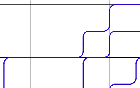
An example of an element of $\mathrm{OP}(4,6,\{1,2,3\},\{1,4,5\},11)$ is $P=\Bigl(\Bigl((4,1)$, $(3,1)$, $(3,2)$, $(3,3)$, $(3,4)$, $(2,4)$, $(2,5)$, $(1,5)$, $(1,6)\Bigr)$, $\Bigl((4,4)$, $(3,4)$, $(3,5)$, $(2,5)$, $(2,6)\Bigr),$ $\Bigl((4,5)$, $(4,6)$, $(3,6)\Bigr)\Bigr)$, which is shown diagrammatically in Figure 2.

For this case, $N(P)=\{(1,1)$, $(1,2)$, $(1,3)$, $(1,4)$, $(2,1)$, $(2,2)$, $(2,3)$, $(4,2)$, $(4,3)\}$, $X(P)=\{(2,5),$ $(3,4)\}$ and $\chi(P)=2$. This will serve as a running example throughout this paper.

In this section, it will be seen that each tuple of osculating paths corresponds naturally to a pair $(H,V)$ of $\{0,1\}$ matrices, which will be referred to as horizontal and vertical edge matrices.

For $P\in\mathrm{OP}(a,b,\alpha,\beta)$, the correspondence is given simply by the rule that $H_{ij}$ is $0$ or $1$ according to whether or not $P$ contains a path which passes from $(i,j)$ to $(i,j\!+\!1)$, and that $V_{ij}$ is $0$ to $1$ according to whether or not $P$ contains a path which passes from $(i\!+\!1,j)$ to $(i,j)$. Thus $H_{ij}$ is associated with the horizontal lattice edge between $(i,j)$ and $(i,j\!+\!1)$, and $V_{ij}$ is associated with the vertical lattice edge between $(i,j)$ and $(i\!+\!1,j)$. It is also convenient to consider boundary edges horizontally between $(i,0)$ and $(i,1)$, and between $(i,b)$ and $(i,b\!+\!1)$, for each $i\in[a]$, and vertically between $(0,j)$ and $(1,j)$, and between $(a,j)$ and $(a\!+\!1,j)$, for each $j\in[b]$, and to include in each path $P_{k}$ the additional points $(a\!+\!1,\beta_{k})$ at the start and $(\alpha_{k},b\!+\!1)$ at the end. Each point $(i,j)\in[a]\!\times\![b]$ can then be associated with a vertex configuration which involves the four values $H_{i,j\!-\!1}$, $V_{ij}$, $H_{ij}$ and $V_{i\!-\!1,j}$, this being depicted diagrammatically as

It can be seen that for any tuple of osculating paths there are only six possible path configurations surrounding any lattice point, given diagrammatically as:

(10)

Correspondingly, there are six possible vertex configurations:

The numbers below each vertex configuration will be used to label the six possible types. Thus, type 1 corresponds to an osculation, and type 2 to a vacancy.

It can also be seen that the six cases of (11) correspond exactly to the simple but important condition

for each $(i,j)\in[a]\!\times\![b]$.

Accordingly, taking into account all of the previous considerations, sets of edge matrix pairs for $a,b\in{P}$ and $(\alpha,\beta)\in\mathrm{BP}(a,b)$ are defined as

and

It can be seen that the ‘boundary conditions’ on $(H,V)\in\mathrm{EM}(a,b,\alpha,\beta)$ are that the first column of $H$ and first row of $V$ are zero, and that the last column of $H$ and last row of $V$ are specified by $\alpha$ and $\beta$ respectively.

As already indicated, for any $P=(P_{1},\ldots,P_{r})\in\mathrm{OP}(a,b,\alpha,\beta)$, a corresponding $(H,V)\in\mathrm{EM}(a,b,\alpha,\beta)$ is given by

and it can be seen straightforwardly that this mapping is a bijection between $\mathrm{OP}(a,b,$ $\alpha,\beta)$ and $\mathrm{EM}(a,b,\alpha,\beta)$.

It can also be seen that the number of osculations of $P$ can be expressed in terms of the corresponding $(H,V)$ as

since $(i,j)$ is an osculation if and only if $H_{i,j\!-\!1}=V_{ij}=1$, or equivalently $V_{i\!-\!1,j}=H_{ij}=1$.

Returning to the running example, the edge matrices are

The edge matrix representation of osculating paths corresponds to the standard representation of configurations of the six-vertex or square ice lattice model in statistical mechanics (see for example [5, Ch. 8] and references therein). In this model $H_{ij}=0$ is represented by a leftward arrow on the corresponding lattice edge, $H_{ij}=1$ by a rightward arrow, $V_{ij}=0$ by a downward arrow, and $V_{ij}=1$ by an upward arrow. The osculating paths then follow the rightward and upward arrows, and condition (12) corresponds to arrow conservation at each lattice point (i.e., the numbers of arrows into and out of each point are equal). One of the main quantities of interest for such statistical mechanical models is the partition function, which is a certain weighted sum over the configurations of the model. The particular case being considered here is that of configurations of the six-vertex model on an $a$ by $b$ rectangle with fixed boundary conditions in which on the upper boundary all arrows point down, on the left boundary all arrows point left, on the lower boundary arrows point up or down according to whether or not their position is in $\beta$, and on the right boundary arrows point right or left according to whether or not their position is in $\alpha$. Note that the six-vertex model has been extensively studied with a variety of boundary conditions. See for example [5, Ch. 8 & 9] for the details of studies with periodic (i.e., toroidal) boundary conditions, and [4, 31, 42, 61, 64] for some studies with other boundary conditions.

In this section, it will be seen that each tuple of osculating paths also corresponds naturally to a $\{-1,0,1\}$ matrix, which will be referred to as an alternating sign matrix. Although this representation of osculating paths will not be used in obtaining any of the results of this paper, it is introduced here in order to present some known formulae for the cardinality of special cases of $\mathrm{OP}(a,b,\alpha,\beta)$ which are usually given in the context of such a representation. Also, as indicated in Section 1, much of the motivation for the work reported in this paper was derived from the studies of alternating sign matrices in which these formulae were obtained. Note, however, that the enumeration results obtained later in this paper apply to cases of $\mathrm{OP}(a,b,\alpha,\beta,l)$, i.e., for which the path tuples all have $l$ vacancy-osculations, whereas the enumeration formulae listed in this section apply to certain cases of $\mathrm{OP}(a,b,\alpha,\beta)$, i.e., for which there is no restriction on the number of vacancy-osculations. Note also that the alternating sign matrices defined in other papers comprise a special case of the alternating sign matrices defined here, and so will be referred to here as ‘standard alternating sign matrices’.

For any $a,b\in{P}$ and $(\alpha,\beta)\in\mathrm{BP}(a,b)$ define the associated set of alternating sign matrices as

For any $(H,V)\in\mathrm{EM}(a,b,\alpha,\beta)$, a corresponding $A\in\mathrm{ASM}(a,b,\alpha,\beta)$ is given simply by

or equivalently, due to (12),

for each $(i,j)\in[a]\!\times\![b]$ (i.e., $A$ is the column difference matrix of $H$ and row difference matrix of $V$). Note that under this mapping vertex configurations 1–4 of (11) at $(i,j)$ give $A_{ij}=0$, configuration 5 gives $A_{ij}=-1$ and configuration 6 gives $A_{ij}=1$.

It can be checked that the mapping (19,20) is a bijection between $\mathrm{EM}(a,b,\alpha,\beta)$ and $\mathrm{ASM}(a,b,\alpha,\beta)$, and that the inverse mapping is

(i.e., $H$ and $V$ are respectively the partial column and row sum matrices of $A$).

It follows, using (16) and (21), that the number of osculations of any $P\in\mathrm{OP}(a,b)$ can be expressed in terms of the corresponding $A\in\mathrm{ASM}(a,b)$ as

The alternating sign matrix for the running example is

Five previously-studied cases of alternating sign matrices will now be considered, for any $n\in{P}$:
$\;\;\bullet\;\;\mathrm{ASM}(n,n,[n],[n])$
$\;\;\bullet\;\;\mathrm{ASM}(n,n\!+\!1,[n],[n\!+\!1]\!\setminus\!\{n\!+\!1\!-\!m\})$, for $m\in[0,n]$
$\;\;\bullet\;\;\mathrm{ASM}(n,n\!+\!m,[n],[n\!-\!1]\cup\{n\!+\!m\})$, for $m\in{N}$
$\;\;\bullet\;\;\mathrm{ASM}(n,2n\!-\!1,[n],\{1,3,5,\ldots,2n\!-\!1\})$
$\;\;\bullet\;\;\mathrm{ASM}(n,n,\{1,3,5,\ldots,2\lceil\frac{n}{2}\rceil\!-\!1\},\{1,3,5,\ldots,2\lceil\frac{n}{2}\rceil\!-\!1\})$
It can be seen that the third case reduces to the first case for $m=0$.

The elements of $\mathrm{ASM}(n,n,[n],[n])$ will be referred to here as standard alternating sign matrices. They are simply $n\!\times\!n$ $\{-1,0,1\}$ matrices in which along each row and column the sum of entries is 1, and the nonzero entries alternate in sign. They were introduced in [38, 39], in which an enumeration formula was conjectured which gives

This was eventually proved in [62] and, using a different method, [35]. The correspondence between standard alternating sign matrices and edge matrices was first identified in [47], and is also discussed, at least in the statistical mechanical model version, in [8, 19, 44]. The correspondence between standard alternating sign matrices and osculating paths is also considered in [8, Sec. 5], [9, Sec. 2], [18, Sec. 9] and [59, Sec. IV].

The six-vertex model boundary conditions for this case, in which all arrows on the upper and lower boundaries point into the square, and all arrows on the left and right boundaries point out of the square, are known as domain wall boundary conditions (see for example [31]).

It can be seen that the $n\!\times\!n$ permutation matrices are included in $\mathrm{ASM}(n,n,[n],[n])$, and, from (22), that if $A$ is a permutation matrix which corresponds to $P\in\mathrm{OP}(n,n,[n],[n])$, then the number of osculations $\chi(P)$ is simply the inversion number of $A$. The inversion number of any $A\in\mathrm{ASM}(a,b)$ could be defined as $\mathcal{I}(A)=\rule[-8.61108pt]{0.0pt}{8.61108pt}\sum_{\{(i,i^{\prime}\!,j,j^{\prime})\in[a]^{2}\!\times\![b]^{2}\,|\,i^{\prime}>i,\;j^{\prime}<j\}}A_{ij}\,A_{i^{\prime}j^{\prime}}$, this being consistent with a definition of inversion number for standard alternating sign matrices given in [39]. It then follows (see for example [47, Theorem 2c]) that $\mathcal{I}(A)=\chi(P)+\mu(A)$, where $P\in\mathrm{OP}(a,b)$ corresponds to $A$, and $\mu(A)$ is the number of $-1$ entries in $A$.

It can be seen that in any standard alternating sign matrix, there is a single 1 in each of the first and last row and column. Furthermore, using elementary symmetry considerations, it follows that the number of $(n\!+\!1)\!\times\!(n\!+\!1)$ standard alternating sign matrices $A$ with $A_{ij}=1$ is the same for $(i,j)$ taken to be any of the eight cases $(1,m\!+\!1)$, $(1,n\!+\!1\!-\!m)$, $(m\!+\!1,1)$, $(n\!+\!1\!-\!m,1)$, $(m\!+\!1,n\!+\!1)$, $(n\!+\!1\!-\!m,n\!+\!1)$, $(n\!+\!1,m\!+\!1)$ or $(n\!+\!1,n\!+\!1\!-\!m)$, for fixed $m\in[0,n]$. Focussing on the case $(n\!+\!1,n\!+\!1\!-\!m)$, i.e., matrices with the 1 of their last row in column $n\!+\!1\!-\!m$, so that $A_{n\!+\!1,j}=\delta_{j,n\!+\!1\!-\!m}$, it follows from (21) that $H_{n\!+\!1,j}=\delta_{j\geq n\!+\!1\!-\!m}$, and then from $V_{n\!+\!1,j}=1$ and (12) that $V_{nj}=\delta_{j\neq n\!+\!1\!-\!m}$, which implies that the submatrices formed by the first $n$ rows of such $A$ comprise $\mathrm{ASM}(n,n\!+\!1,[n],[n\!+\!1]\!\setminus\!\{n\!+\!1\!-\!m\})$. Obtaining the cardinality of this and the seven related sets is known as refined alternating sign matrix enumeration, and, following conjectures in [38, 39], was achieved in [63] and more recently in [15, 21] giving

The related case of $\mathrm{ASM}(n,n\!+\!m,[n],[n\!-\!1]\!\cup\!\{n\!+\!m\})$ was considered in [21], in which an enumeration formula gives

A matrix is horizontally-symmetric if it is invariant under reflection about the horizontal line through its center, and horizontally-and-vertically symmetric if it is invariant under reflection about both the horizontal and vertical lines through its center. It can be seen that for standard alternating sign matrices, such symmetries can only occur for odd-sized matrices.

Considering horizontally-symmetric $(2n\!+\!1)\!\times\!(2n\!+\!1)$ standard alternating sign matrices $A$, i.e., those for which $A_{ij}=A_{2n\!+\!2\!-\!i,j}$ for each $(i,j)\in[2n\!+\!1]\!\times\![2n\!+\!1]$, it can be seen that the first and last columns always have their $1$’s in the middle row, $A_{i1}=A_{i,2n\!+\!1}=\delta_{i,n\!+\!1}$, and that the middle row always consists entirely of alternating $1$’s and $-1$’s, $A_{n\!+\!1,j}=(-1)^{j\!+\!1}$. Proceeding to the corresponding edge matrices, it is then found that along the first column of vertices $H_{i0}=0$, $V_{i1}=\delta_{i\geq n\!+\!1}$ and $H_{i1}=\delta_{i,n\!+\!1}$, along the last column of vertices $H_{i,2n}=\delta_{i\neq n\!+\!1}$, $V_{i,2n\!+\!1}=\delta_{i\geq n\!+\!1}$ and $H_{i,2n\!+\!1}=1$, and along the middle row of vertices $V_{nj}=\delta_{j\;\mathrm{even}}$, $H_{n\!+\!1,j}=\delta_{j\;\mathrm{odd}}$ and $V_{n\!+\!1,j}=\delta_{j\;\mathrm{odd}}$. It follows that each such $A$ is uniquely determined by the submatrix formed by the first $n$ rows of $A$ with their first and last columns deleted (i.e., $A_{ij}$ with $(i,j)\in[n]\!\times\![2,2n]$), and that these submatrices comprise $\mathrm{ASM}(n,2n\!-\!1,[n],\{1,3,\ldots,2n\!-\!1\})$. Following conjectures in [45, 46], an enumeration formula was proved in [36] giving

Considering horizontally-and-vertically-symmetric $(2n\!+\!3)\!\times\!(2n\!+\!3)$ standard alternating sign matrices $A$, i.e., those for which $A_{ij}=A_{2n\!+\!4\!-\!i,j}=A_{i,2n\!+\!4\!-\!j}$ for each $(i,j)\in[2n\!+\!3]\!\times\![2n\!+\!3]$, it follows, since both $A$ and $A^{t}$ are horizontally symmetric, that each such $A$ is uniquely determined by the submatrix formed by $A_{ij}$ with $(i,j)\in[2,n\!+\!1]\!\times\![2,n\!+\!1]$, and that these submatrices comprise $\mathrm{ASM}(n,n,\{1,3,\ldots,2\lceil\frac{n}{2}\rceil\!-\!1\},\{1,3,\ldots,2\lceil\frac{n}{2}\rceil\!-\!1\})$. Following conjectures in [45, 46], an enumeration formula was proved in [41] giving

In this section, the vacancy-osculation set $Z(P)$ associated with each path tuple $P\in\mathrm{OP}(a,b)$ will be studied further, and it will be shown that, for fixed $a$ and $b$, $P$ is uniquely determined by $Z(P)$.

For any $a,b\in{P}$, $(\alpha,\beta)\in\mathrm{BP}(a,b)$ and $l\in{N}$, define sets of vacancy-osculation sets as

References

- [1] G. Andrews Invent. Math. 53 (1979) 193–225 Plane Partitions III: The Weak Macdonald Conjecture
- [2] G. Andrews J. Combin. Theory Ser. A 66 (1994) 28–39 Plane Partitions V: The TSSCPP Conjecture
- [3] T. H. Baker and P. J. Forrester J. Phys. A 34 (2001) L381–L390 Random Walks and Random Fixed-Point Free Involutions
- [4] M. T. Batchelor, R. J. Baxter, M. J. O’Rourke and C. M. Yung J. Phys. A 28 (1995) 2759–2770 Exact Solution and Interfacial Tension of the Six-Vertex Model with Anti-Periodic Boundary Conditions
- [5] R. J. Baxter Exactly Solved Models in Statistical Mechanics (Academic Press, 1982)
- [6] A. Berele J. Combin. Theory Ser. A 43 (1986) 320–328 A Schensted-Type Correspondence for the Symplectic Group
- [7] M. Bousquet-Mélou J. Phys. Conference Series 42 (2006) 35–46 Three Osculating Walkers
- [8] M. Bousquet-Mélou and L. Habsieger Discrete Math. 139 (1995) 57–72 Sur les Matrices à Signes Alternants
- [9]
R. Brak Osculating Lattice Paths and Alternating Sign Matrices in
Proceedings of 9th Formal Power Series and Algebraic Combinatorics Conference (Vienna, 1997) Available at
http://www.ms.unimelb.edu.au/
~brak/publications.html - [10] D. M. Bressoud Proofs and Confirmations: The Story of the Alternating Sign Matrix Conjecture (Cambridge University Press, 1999)
- [11] D. M. Bressoud and J. Propp Notices Amer. Math. Soc. 46 (1999) 637–646 How the Alternating Sign Matrix Conjecture was Solved
- [12] W. H. Burge J. Combin. Theory Ser. A 17 (1974) 12–30 Four Correspondences Between Graphs and Generalized Young Tableaux
- [13] C. Chauve and S. Dulucq Discrete Math. 246 (2002) 67–81 A Geometric Version of the Robinson-Schensted Correspondence for Skew Oscillating Tableaux
- [14] S. H. Choi Honam Math. J. 25 (2003) 3–15 An Analogue of Robinson-Schensted Correspondence for Oscillating Generalized Tableaux
- [15] F. Colomo and A. G. Pronko J. Stat. Mech. (2005) P01005 33pp. Square Ice, Alternating Sign Matrices and Classical Orthogonal Polynomials
- [16] M. P. Delest, S. Dulucq and L. Favreau Sém. Lothar. Combin. 20 (1988) B20b 14pp. An Analogue to Robinson-Schensted Correspondence for Oscillating Tableaux
- [17] S. Dulucq and B. Sagan Discrete Math. 139 (1995) 129–142 La Correspondance de Robinson-Schensted pour les Tableaux Oscillants Gauches
- [18] O. Eğecioğlu, T. Redmond and C. Ryavec Electron. J. Combin. 8 (2001) R36 51pp. From a Polynomial Riemann Hypothesis to Alternating Sign Matrices
- [19] N. Elkies, G. Kuperberg, M. Larsen and J. Propp J. Algebraic Combin. 1 (1992) 111–132 & 219–234 Alternating-Sign Matrices and Domino Tilings (Parts I & II)
- [20] J. Essam J. Stat. Phys. 110 (2003) 1191–1207 Three Attractive Osculating Walkers and a Polymer Collapse Transition
- [21] I. Fischer J. Combin. Theory Ser. A 114 (2007) 253–264 A New Proof of the Refined Alternating Sign Matrix Theorem
- [22] W. Fulton Young Tableaux (Cambridge University Press, 1997)
- [23] I. M. Gessel J. Statist. Plann. Inference 34 (1993) 125–134 Counting Paths in Young’s Lattice
- [24] I. M. Gessel and X. G. Viennot Adv. Math. 58 (1985) 300–321 Binomial Determinants, Paths and Hook Length Formulae
- [25]
I. M. Gessel and X. G. Viennot Determinants, Paths and Plane Partitions (1989) Available at
http://people.brandeis.edu/
~gessel/homepage/papers
/pp.pdf - [26] I. M. Gessel and G. Xin Electron. J. Combin. 13 (2006) R53 48pp. The Generating Function of Ternary Trees and Continued Fractions
- [27] A. Goupil and C. Chauve Sém. Lothar. Combin. 54 (2006) B54j 13pp. Combinatorial Operators for Kronecker Powers of Representations of
- [28] A. J. Guttmann and M. Vöge J. Statist. Plann. Inference 101 (2002) 107–131 Lattice Paths: Vicious Walkers and Friendly Walkers
- [29] M. Ishikawa arXiv:math.CO/0602068 On Refined Enumerations of Totally Symmetric Self-Complementary Plane Partitions I
- [30] M. Ishikawa arXiv:math.CO/0606082 On Refined Enumerations of Totally Symmetric Self-Complementary Plane Partitions II
- [31] A. G. Izergin, D. A. Coker and V. E. Korepin J. Phys. A 25 (1992) 4315–4334 Determinant Formula for the Six-Vertex Model
- [32] C. Krattenthaler J. Statist. Plann. Inference 54 (1996) 75–85 Oscillating Tableaux and Nonintersecting Lattice Paths
- [33] C. Krattenthaler European J. Combin. 27 (2006) 1138–1146 Descending Plane Partitions and Rhombus Tilings of a Hexagon with Triangular Hole
- [34] C. Krattenthaler, A. J. Guttmann and X. G. Viennot J. Stat. Phys. 110 (2003) 1069–1086 Vicious Walkers, Friendly Walkers and Young Tableaux III: Between Two Walls
- [35] G. Kuperberg Int. Math. Res. Not. (1996) 139–150 Another Proof of the Alternating-Sign Matrix Conjecture
- [36] G. Kuperberg Ann. of Math. 156 (2002) 835–866 Symmetry Classes of Alternating-Sign Matrices under One Roof
- [37] P. Lalonde Discrete Math. 271 (2003) 311–319 Lattice Paths and the Antiautomorphism of the Poset of Descending Plane Partitions
- [38] W. H. Mills, D. P. Robbins and H. Rumsey Invent. Math. 66 (1982) 73–87 Proof of the Macdonald Conjecture
- [39] W. H. Mills, D. P. Robbins and H. Rumsey J. Combin. Theory Ser. A 34 (1983) 340–359 Alternating Sign Matrices and Descending Plane Partitions
- [40] W. H. Mills, D. P. Robbins and H. Rumsey J. Combin. Theory Ser. A 42 (1986) 277–292 Self-Complementary Totally Symmetric Plane Partitions
- [41] S. Okada J. Algebraic Combin. 23 (2006) 43–69 Enumeration of Symmetry Classes of Alternating Sign Matrices and Characters of Classical Groups
- [42] A. L. Owczarek and R. J. Baxter J. Phys. A 22 (1989) 1141–1165 Surface Free Energy of the Critical Six-Vertex Model with Free Boundaries
- [43] R. A. Proctor Trans. Amer. Math. Soc. 324 (1991) 655–692 A Generalized Berele-Schensted Algorithm and Conjectured Young Tableaux for Intermediate Symplectic Groups
- [44] J. Propp Discrete Math. Theor. Comput. Sci. Proceedings AA (DM-CCG) (2001) 43–58 The Many Faces of Alternating-Sign Matrices
- [45] D. P. Robbins Math. Intelligencer 13 (1991) 12–19 The Story of 1, 2, 7, 42, 429, 7436,…
- [46] D. P. Robbins arXiv:math.CO/0008045 Symmetry Classes of Alternating Sign Matrices
- [47] D. P. Robbins and H. Rumsey Adv. Math. 62 (1986) 169–184 Determinants and Alternating Sign Matrices
- [48] T. Roby Applications and Extensions of Fomin’s Generalization of the Robinson-Schensted Correspondence to Differential Posets (1991) PhD Thesis, Massachusetts Institute of Technology
- [49] T. Roby Discrete Math. 139 (1995) 481–485 The Connection Between the Robinson-Schensted Correspondence for Skew Oscillating Tableaux and Graded Graphs
- [50] T. Roby and I. Terada Electron. J. Combin. 12 (2005) R4 42 pp. A Two-Dimensional Pictorial Presentation of Berele’s Insertion Algorithm for Symplectic Tableaux
- [51] B. E. Sagan The Ubiquitous Young Tableau in Invariant Theory and Tableaux (Minneapolis, 1998) IMA Vol. Math. Appl. 19 (1990) 262-298
- [52] B. E. Sagan The Symmetric Group: Representations, Combinatorial Algorithms and Symmetric Functions (Second Edition) (Springer, 2001)
- [53] R. P. Stanley Enumerative Combinatorics: Volume 1 (Cambridge University Press, 1986)
- [54] R. P. Stanley Enumerative Combinatorics: Volume 2 (Cambridge University Press, 1999)
- [55] R. P. Stanley Increasing and Decreasing Subsequences and Their Variants in Proceedings of International Congress of Mathematicians (Madrid, 2006)
- [56] J. R. Stembridge Adv. Math. 83 (1990) 96–131 Nonintersecting Paths, Pfaffians and Plane Partitions
- [57] S. Sundaram On the Combinatorics of Representations of (1986) Massachusetts Institute of Technology, PhD Thesis
- [58] S. Sundaram J. Combin. Theory Ser. A 53 (1990) 209–238 The Cauchy Identity for
- [59] U. Tamm Electron. J. Combin. 8 (2001) A1 31pp. Some Aspects of Hankel Matrices in Coding Theory and Combinatorics
- [60] I. Terada J. Algebraic Combin. 14 (2001) 229–267 Brauer Diagrams, Updown Tableaux and Nilpotent Matrices
- [61] C. M. Yung and M. T. Batchelor Nuclear Phys. B 435 (1995) 430–462 Integrable Vertex and Loop Models on the Square Lattice with Open Boundaries via Reflection Matrices
- [62] D. Zeilberger Electron. J. Combin. 3 (1996) R13 84pp. Proof of the Alternating Sign Matrix Conjecture
- [63] D. Zeilberger New York J. Math. 2 (1996) 59–68 Proof of the Refined Alternating Sign Matrix Conjecture
- [64] P. Zinn-Justin arXiv:cond-mat/0205192 The Influence of Boundary Conditions in the Six-Vertex Model