跳到论文正文
W Papers独立论文阅读器 arXiv:math/0701583 论文正文 计算阅读时间 · 0%
引用这篇论文根据当前论文元数据生成,正式投稿前建议核对。


License: Assumed arXiv.org perpetual non-exclusive license
arXiv:math/0701583v1 [math.ST] 21 Jan 2007

Bayesian shrinkage prediction for the regression problem

Kei Kobayashi Note: kei@ism.ac.jp    Fumiyasu Komaki Note: komaki@mist.i.u-tokyo.ac.jp
Abstract

We consider Bayesian shrinkage predictions for the Normal regression problem under the frequentist Kullback-Leibler risk function.

Firstly, we consider the multivariate Normal model with an unknown mean and a known covariance. While the unknown mean is fixed, the covariance of future samples can be different from training samples. We show that the Bayesian predictive distribution based on the uniform prior is dominated by that based on a class of priors if the prior distributions for the covariance and future covariance matrices are rotation invariant.

Then, we consider a class of priors for the mean parameters depending on the future covariance matrix. With such a prior, we can construct a Bayesian predictive distribution dominating that based on the uniform prior.

Lastly, applying this result to the prediction of response variables in the Normal linear regression model, we show that there exists a Bayesian predictive distribution dominating that based on the uniform prior. Minimaxity of these Bayesian predictions follows from these results.

Key words: Bayesian prediction, shrinkage estimation, Normal regression, superharmonic function, minimaxity, Kullback-Leibler divergence.

1 Introduction

Suppose that we have observations y∼Nd​(y,μ,Σ)y\sim N_{d}(y;\mu,\Sigma). Here NdN_{d} is the density function of the dd-dimensional multivariate Normal distribution with mean vector μ\mu and covariance matrix Σ\Sigma. We consider the prediction of y~∼Nd​(y~,μ,Σ~)\tilde{y}\sim N_{d}(\tilde{y};\mu,\tilde{\Sigma}) using a predictive density p^​(y~|y).\hat{p}(\tilde{y}|y). We assume that the mean of the distribution of unobserved (future) samples is the same as the one of the observed samples. However, the covariance matrices, Σ\Sigma and Σ~\tilde{\Sigma}, are not necessarily the same or proportional to each other. We call a problem with such settings the “problem with changeable covariances.” As we will show below, the changeable covariance is a natural assumption when we consider the linear regression problems.

In the present work, we assume that the mean vector μ\mu is unknown and the covariance matrix Σ\Sigma is known. We consider both cases where the future covariance Σ~\tilde{\Sigma} is known and unknown.

We evaluate predictive densities p^​(y~|y)\hat{p}(\tilde{y}|y) by the KL loss function

D(p~(y~|θ)∥p^(y~|y)):=∫p~(y~|θ)logp~​(y~|θ)p^​(y~|y)dy~D(\tilde{p}(\tilde{y}|\theta)\|\hat{p}(\tilde{y}|y)):=\int\tilde{p}(\tilde{y}|\theta)\log\frac{\tilde{p}(\tilde{y}|\theta)}{\hat{p}(\tilde{y}|y)}\mathrm{d}\tilde{y} (1)

and the (frequentist) risk function

RKL(p^,θ):=∫p(y|θ)D(p~(y~|θ)∥p^(y~|y))dy~.R_{\rm KL}(\hat{p},\theta):=\int p(y|\theta)D(\tilde{p}(\tilde{y}|\theta)\|\hat{p}(\tilde{y}|y))\mathrm{d}\tilde{y}. (2)

We consider the Bayesian predictive density

pπ​(y~|y):=∫p~​(y~|θ)​p​(y|θ)​π​(θ)​𝑑θ∫p⁡(y|θ)​π​(θ)​𝑑θp_{\pi}(\tilde{y}|y):=\frac{\int\tilde{p}(\tilde{y}|\theta)p(y|\theta)\pi(\theta)\mathrm{d}\theta}{\int p(y|\theta)\pi(\theta)\mathrm{d}\theta}

with prior π⁡(θ)\pi(\theta). For the Normal model, the Bayesian predictive density with the uniform prior πI​(μ)=1\pi_{I}(\mu)=1 becomes

pπ​(y~|y;Σ,Σ~)=1(2​π)d/2​|Σ+Σ~|1/2​exp⁡(−(y~−y)⊤​(Σ+Σ~)−1​(y~−y)2),p_{\pi}(\tilde{y}|y;\Sigma,\tilde{\Sigma})=\frac{1}{(2\pi)^{d/2}|\Sigma+\tilde{\Sigma}|^{1/2}}\exp\Big(-\frac{(\tilde{y}-y)^{\top}(\Sigma+\tilde{\Sigma})^{-1}(\tilde{y}-y)}{2}\Big),

as we will see in Section 2. Let pπ​(y~|y;Σ,Σ~)p_{\pi}(\tilde{y}|y;\Sigma,\tilde{\Sigma}) denote pπ​(y~|y)p_{\pi}(\tilde{y}|y) for short.

When Σ~\tilde{\Sigma} is proportional to Σ\Sigma, i.e. Σ~=a​Σ\tilde{\Sigma}=a\Sigma for a>0a>0, the problem is reduced to the one with Σ=v​Id\Sigma=vI_{d} and Σ~=v~​Id\tilde{\Sigma}=\tilde{v}I_{d} for positive scalar values vv and v~\tilde{v}. This case with ‘unchangeable covariances’ has been well studied. The Bayesian predictive density

pI​(y~|y;Σ,Σ~)=1{2​π​(v+v~)}d/2​exp⁡(−‖y~−y‖22​(v+v~))p_{I}(\tilde{y}|y;\Sigma,\tilde{\Sigma})=\frac{1}{\{2\pi(v+\tilde{v})\}^{d/2}}\exp\Big(-\frac{\|\tilde{y}-y\|^{2}}{2(v+\tilde{v})}\Big)

based on the uniform prior πI​(μ)=1\pi_{\rm I}(\mu)=1 dominates the plug-in density

p⁡(y~|μ^)=1{2​π​v~}d/2​exp⁡(−‖y~−y‖22​v~)p(\tilde{y}|\hat{\mu})=\frac{1}{\{2\pi\tilde{v}\}^{d/2}}\exp\Big(-\frac{\|\tilde{y}-y\|^{2}}{2\tilde{v}}\Big)

with MLE, where μ^=y\hat{\mu}=y. Moreover, by Murray 1977 and Ng 1980, the Bayesian predictive density pI​(y~|y)p_{\rm I}(\tilde{y}|y) is the best predictive density that is invariant under the translation group. In Liang & Barron 2004 and George et al. 2006, the minimaxity of pIp_{\rm I} was proved.

In Komaki 2001, it was proved that the Bayesian predictive density pS​(y~|y)p_{\rm S}(\tilde{y}|y) with Stein prior

πS​(μ):=‖μ‖−(d−2)\pi_{\rm S}(\mu):=\|\mu\|^{-(d-2)} (3)

dominates the Bayesian predictive density pI​(y~|y)p_{\rm I}(\tilde{y}|y) with the uniform prior πI​(μ)\pi_{\rm I}(\mu).

George et al. 2006 generalized the result of Komaki 2001. Define the marginal distribution mπm_{\pi} by

mπ​(z,Σ):=∫N⁡(z,μ,Σ)​π​(μ)​𝑑μ.m_{\pi}(z;\Sigma):=\int{\rm N}(z;\mu,\Sigma)\pi(\mu)\,\mathrm{d}\mu. (4)

As we will see in Theorem 2.4 below, George et al. 2006 proved a sufficient condition on the prior π⁡(μ)\pi(\mu) or the marginal distribution mπm_{\pi} for pπ​(y~|y)p_{\pi}(\tilde{y}|y) to dominate pI​(y~|y)p_{\rm I}(\tilde{y}|y) when Σ\Sigma is proportional to Σ~\tilde{\Sigma}. In the present work, we generalize the results of Komaki 2001 and George et al. 2006 to the corresponding problem with the changeable covariances, considering only finite sample cases. Asymptotic properties of Bayesian prediction are studied in Komaki 1996, Corcuera & Giummolé 2000, and Komaki 2006.

2 Prior distributions independent of the future covariance

In this section, we develop and prove our main results concerning properties of pπ​(y~|y)p_{\pi}(\tilde{y}|y) in the problem with changeable covariances.

First we give three lemmas generalizing results proved in George et al. 2006 for the problem with “unchangeable” variances.

Define the marginal distribution mπm_{\pi} by (4).

Lemma 2.1

If mπ​(z,Σ)<∞m_{\pi}(z;\Sigma)<\infty for all zz, then pπ​(y~|y)p_{\pi}(\tilde{y}|y) is a proper probability density. Moreover, the mean of pπ​(y~|y)p_{\pi}(\tilde{y}|y) is equal to the posterior mean Eπ​[μ|y]E_{\pi}[\mu|y] if it exists.

Let

w:=(Σ−1+Σ~−1)−1​(Σ−1​y+Σ~−1​y~)w:=(\Sigma^{-1}+\tilde{\Sigma}^{-1})^{-1}(\Sigma^{-1}y+\tilde{\Sigma}^{-1}\tilde{y})

and

Σw:=(Σ−1+Σ~−1)−1.\Sigma_{w}:=(\Sigma^{-1}+\tilde{\Sigma}^{-1})^{-1}. (5)

As a function of the predictive density based on the uniform prior, the Bayesian predictive density based on a prior π⁡(μ)\pi(\mu) becomes as follows:

Lemma 2.2
pπ​(y~|y)=pI​(y~|y)​mπ​(w,Σw)mπ​(y,Σ).p_{\pi}(\tilde{y}|y)=p_{\rm I}(\tilde{y}|y)\frac{m_{\pi}(w;\Sigma_{w})}{m_{\pi}(y;\Sigma)}.

The following lemma is used for proving minimaxity of pπ​(y~|y)p_{\pi}(\tilde{y}|y).

Lemma 2.3

The Bayesian predictive density pI​(y~|y)p_{I}(\tilde{y}|y) is minimax under KL risk function RKL​(p^,μ)R_{\rm KL}(\hat{p},\mu).

Since the proofs of Lemma 2.1 and Lemma 2.3 are almost same as those of Lemma 1 and Lemma 3 in George et al. 2006, we omit them. We prove only Lemma 2.2.

Proof of Lemma 2.2

p(y|\displaystyle p(y| OPENμ,Σ)​p​(y~|μ,Σ~)\displaystyle\mu,\Sigma)p(\tilde{y}|\mu,\tilde{\Sigma})
=1(2​π)d/2​|Σ|1/2​exp⁡(−(y−μ)⊤​Σ−1​(y−μ)2)​1(2​π)d/2​|Σ~|1/2​exp⁡(−(y~−μ)⊤​Σ~−1​(y~−μ)2)\displaystyle=\frac{1}{(2\pi)^{d/2}|\Sigma|^{1/2}}\exp\Big(-\frac{(y-\mu)^{\top}\Sigma^{-1}(y-\mu)}{2}\Big)\frac{1}{(2\pi)^{d/2}|\tilde{\Sigma}|^{1/2}}\exp\Big(-\frac{(\tilde{y}-\mu)^{\top}\tilde{\Sigma}^{-1}(\tilde{y}-\mu)}{2}\Big)
=1(2​π)d/2​|Σ|1/2​1(2​π)d/2​|Σ~|1/2​exp⁡(−(w−μ)⊤​Σw−1​(w−μ)2)​exp⁡(−y⊤​Σ−1​y2−y~⊤​Σ~−1​y~2)\displaystyle=\frac{1}{(2\pi)^{d/2}|\Sigma|^{1/2}}\frac{1}{(2\pi)^{d/2}|\tilde{\Sigma}|^{1/2}}\exp\Big(-\frac{(w-\mu)^{\top}\Sigma_{w}^{-1}(w-\mu)}{2}\Big)\exp\Big(-\frac{y^{\top}\Sigma^{-1}y}{2}-\frac{\tilde{y}^{\top}\tilde{\Sigma}^{-1}\tilde{y}}{2}\Big)
exp⁡((Σ−1​y+Σ~−1​y~)⊤​(Σ−1+Σ~−1)−1​(Σ−1​y+Σ~−1​y~)2)\displaystyle~~~~~~~~~~~~~~~~~~~~~~~~~~~~~~~~~~~~~~~~~~~~~~~\exp\Big(\frac{(\Sigma^{-1}y+\tilde{\Sigma}^{-1}\tilde{y})^{\top}(\Sigma^{-1}+\tilde{\Sigma}^{-1})^{-1}(\Sigma^{-1}y+\tilde{\Sigma}^{-1}\tilde{y})}{2}\Big)
=1(2​π)d/2​|Σ|1/2​1(2​π)d/2​|Σ~|1/2​exp⁡(−(w−μ)⊤​Σw−1​(w−μ)2)​exp⁡(−(y−y~)⊤​(Σ+Σ~)−1​(y−y~)2)\displaystyle=\frac{1}{(2\pi)^{d/2}|\Sigma|^{1/2}}\frac{1}{(2\pi)^{d/2}|\tilde{\Sigma}|^{1/2}}\exp\Big(-\frac{(w-\mu)^{\top}\Sigma_{w}^{-1}(w-\mu)}{2}\Big)\exp\Big(-\frac{(y-\tilde{y})^{\top}(\Sigma+\tilde{\Sigma})^{-1}(y-\tilde{y})}{2}\Big) (6)

In the last equation, we use

Σ−1\displaystyle\Sigma^{-1} (Σ−1+Σ~−1)−1​Σ−1−Σ−1\displaystyle(\Sigma^{-1}+\tilde{\Sigma}^{-1})^{-1}\Sigma^{-1}-\Sigma^{-1}
=Σ−1​(Σ−1+Σ~−1)−1​Σ−1−Σ−1​(Σ−1+Σ~−1)−1​(Σ−1+Σ~−1)\displaystyle=\Sigma^{-1}(\Sigma^{-1}+\tilde{\Sigma}^{-1})^{-1}\Sigma^{-1}-\Sigma^{-1}(\Sigma^{-1}+\tilde{\Sigma}^{-1})^{-1}(\Sigma^{-1}+\tilde{\Sigma}^{-1})
=−Σ−1​(Σ−1+Σ~−1)−1​Σ~−1\displaystyle=-\Sigma^{-1}(\Sigma^{-1}+\tilde{\Sigma}^{-1})^{-1}\tilde{\Sigma}^{-1}
=−(Σ+Σ~)−1.\displaystyle=-(\Sigma+\tilde{\Sigma})^{-1}.

From (6), the predictive density with the uniform prior I⁡(μ)=1I(\mu)=1 is given by

pI​(y~|y)\displaystyle p_{\rm I}(\tilde{y}|y) =∫p⁡(y|μ,Σ)​p​(y~|μ,Σ~)​𝑑μ∫p⁡(y|μ,Σ)​𝑑μ\displaystyle=\frac{\int p(y|\mu,\Sigma)p(\tilde{y}|\mu,\tilde{\Sigma})\,\mathrm{d}\mu}{\int p(y|\mu,\Sigma)\,\mathrm{d}\mu}
=1(2​π)d/2​|Σ|1/21(2​π)d/2​|Σ~|1/2|Σ−1+Σ~−1|−1/2(2π)d/2exp(−(y−y~)⊤​(Σ+Σ~)−1​(y−y~)2)\displaystyle=\frac{1}{(2\pi)^{d/2}|\Sigma|^{1/2}}\frac{1}{(2\pi)^{d/2}|\tilde{\Sigma}|^{1/2}}|\Sigma^{-1}+\tilde{\Sigma}^{-1}|^{-1/2}(2\pi)^{d/2}\exp\Big(-\frac{(y-\tilde{y})^{\top}(\Sigma+\tilde{\Sigma})^{-1}(y-\tilde{y})}{2}\Big)
=(2π)−d/2|Σ+Σ~|−1/2exp(−(y−y~)⊤​(Σ+Σ~)−1​(y−y~)2).\displaystyle=(2\pi)^{-d/2}|\Sigma+\tilde{\Sigma}|^{-1/2}\exp\Big(-\frac{(y-\tilde{y})^{\top}(\Sigma+\tilde{\Sigma})^{-1}(y-\tilde{y})}{2}\Big).

Therefore

pπ​(y~|y)\displaystyle p_{\pi}(\tilde{y}|y) =∫p⁡(y|μ,Σ)​p​(y~|μ,Σ~)​π​(μ)​𝑑μ∫p⁡(y|μ,Σ)​π​(μ)​𝑑μ\displaystyle=\frac{\int p(y|\mu,\Sigma)p(\tilde{y}|\mu,\tilde{\Sigma})\pi(\mu)\,\mathrm{d}\mu}{\int p(y|\mu,\Sigma)\pi(\mu)\,\mathrm{d}\mu}
=pI​(y~|y)​∫N⁡(w,μ,Σw)​π​(μ)​𝑑μ∫N⁡(y,μ,Σ)​π​(μ)​𝑑μ\displaystyle=\frac{p_{\rm I}(\tilde{y}|y)\int{\rm N}(w;\mu,\Sigma_{w})\pi(\mu)\,\mathrm{d}\mu}{\int{\rm N}(y;\mu,\Sigma)\pi(\mu)\,\mathrm{d}\mu}
=pI​(y~|y)​mπ​(w,Σw)mπ​(y,Σ).\displaystyle=p_{\rm I}(\tilde{y}|y)\frac{m_{\pi}(w;\Sigma_{w})}{m_{\pi}(y;\Sigma)}.

□\square

Next, the difference of the risk functions of the two priors is evaluated. Let

RKL(π,μ):=∫p(y|μ,Σ)D(p(y~|μ,Σ~)∥pπ(y~|y))dyR_{\rm KL}(\pi,\mu):=\int p(y|\mu,\Sigma)D(p(\tilde{y}|\mu,\tilde{\Sigma})\|p_{\pi}(\tilde{y}|y))\,\mathrm{d}y
ϕπ​(μ,Σ):=∫N⁡(z,μ,Σ)​log⁡mπ​(z,Σ)​𝑑z.\phi_{\pi}(\mu,\Sigma):=\int{\rm N}(z;\mu,\Sigma)\log m_{\pi}(z;\Sigma)\,\mathrm{d}z.

Then from Lemma 2.2,

RKL​(π,μ)−RKL​(πI,μ)\displaystyle R_{\rm KL}(\pi,\mu)-R_{\rm KL}(\pi_{\rm I},\mu) =∫p⁡(y|μ,Σ)​p​(y~|μ,Σ~)​log⁡pI​(y~|y)pπ​(y~|y)​𝑑y​𝑑y~\displaystyle=\int p(y|\mu,\Sigma)p(\tilde{y}|\mu,\tilde{\Sigma})\log\frac{p_{\rm I}(\tilde{y}|y)}{p_{\pi}(\tilde{y}|y)}\,\mathrm{d}y\,\mathrm{d}\tilde{y}
=∫p⁡(y|μ,Σ)​p​(y~|μ,Σ~)​log⁡mπ​(y,Σ)mπ​(w,Σw)​𝑑y​𝑑y~\displaystyle=\int p(y|\mu,\Sigma)p(\tilde{y}|\mu,\tilde{\Sigma})\log\frac{m_{\pi}(y;\Sigma)}{m_{\pi}(w;\Sigma_{w})}\,\mathrm{d}y\,\mathrm{d}\tilde{y}
=ϕπ​(μ,Σ)−ϕπ​(μ,Σw).\displaystyle=\phi_{\pi}(\mu,\Sigma)-\phi_{\pi}(\mu,\Sigma_{w}). (7)

Now Σw=(Σ−1+Σ~−1)−1≺Σ\Sigma_{w}=(\Sigma^{-1}+\tilde{\Sigma}^{-1})^{-1}\prec\Sigma. In order to prove RKL​(π,μ)<RKL​(πI,μ)R_{\rm KL}(\pi,\mu)<R_{\rm KL}(\pi_{\rm I},\mu), it suffices to prove ϕπ​(μ,Σ)<ϕπ​(μ,Σw)\phi_{\pi}(\mu,\Sigma)<\phi_{\pi}(\mu,\Sigma_{w}).

Before stating the main results for the problem with changeable covariances, we review some results with a special setting, i.e., unchangeable covariances.

An extended real-valued function π⁡(μ)\pi(\mu) on an open set R⊂ℝpR\subset\mathbb{R}^{p} is said to be superharmonic when it satisfies the following properties:

  1. 1.

    −∞<π⁡(μ)≤∞-\infty<\pi(\mu)\leq\infty and π⁡(μ)≢∞\pi(\mu)\not\equiv\infty on any component of RR.

  2. 2.

    π⁡(μ)\pi(\mu) is lower semi-continuous on RR.

  3. 3.

    If GG is an open subset of RR with compact closure G¯⊂R\bar{G}\subset R, w⁡(μ)w(\mu) is a continuous function on G¯\bar{G}, w⁡(μ)w(\mu) is harmonic on GG, and π⁡(μ)≥w⁡(μ)\pi(\mu)\geq w(\mu) on ∂G\partial{G}, then π⁡(μ)≥w⁡(μ)\pi(\mu)\geq w(\mu) on GG.

If π⁡(μ)\pi(\mu) is a C2C^{2} function, then π⁡(μ)\pi(\mu) is superharmonic on RR if and only if Δ​π≤0\Delta\pi\leq 0 on RR.

Theorem 2.4 (Komaki 2001 and George et al. 2006)

Assume d≥3d\geq 3.

(i) If π⁡(μ)\pi(\mu) is the Stein prior πS​(μ)\pi_{\rm S}(\mu),

v1>v2>0⇒ϕπ​(μ,v1​Id)<ϕπ​(μ,v2​Id)​ for all ​μ.v_{1}>v_{2}>0\Rightarrow\phi_{\pi}(\mu,v_{1}I_{d})<\phi_{\pi}(\mu,v_{2}I_{d})\mbox{ for all }\mu.

(ii) If π⁡(μ)\pi(\mu) is a superharmonic function and mπ​(z,v​Id)<∞m_{\pi}(z;vI_{d})<\infty for any zz and vv,

v1>v2>0⇒ϕπ​(μ,v1​Id)≤ϕπ​(μ,v2​Id)​ for all ​μ.v_{1}>v_{2}>0\Rightarrow\phi_{\pi}(\mu,v_{1}I_{d})\leq\phi_{\pi}(\mu,v_{2}I_{d})\mbox{ for all }\mu.

Furthermore, if mπ​(z,v​Id)m_{\pi}(z;vI_{d}) is also not constant for all v2≤v≤v1v_{2}\leq v\leq v_{1}, the inequality
        holds strictly.

(iii) If mπ​(z,v​Id)\sqrt{m_{\pi}(z;vI_{d})} is a superharmonic function for any vv and mπ​(z,v​Id)<∞m_{\pi}(z;vI_{d})<\infty for any zz and vv,

v1>v2>0⇒ϕπ​(μ,v1​Id)≤ϕπ​(μ,v2​Id)​ for all ​μ.v_{1}>v_{2}>0\Rightarrow\phi_{\pi}(\mu,v_{1}I_{d})\leq\phi_{\pi}(\mu,v_{2}I_{d})\mbox{ for all }\mu.

Furthermore, if mπ​(z,v​Id)m_{\pi}(z;vI_{d}) is also not constant for any v2≤v≤v1v_{2}\leq v\leq v_{1}, the inequality
        holds strictly.

We note that (iii) implies (ii) and (ii) implies (i). (i) was proved in Komaki 2001. (ii) and (iii) were proved in George et al. 2006.

Theorem 2.5 is a generalization of (ii) of Theorem 2.4 to the problem with changeable covariances. For each prior π⁡(μ)\pi(\mu), define a rescaled prior with respect to a positive definite d×dd\times d matrix Σ∗\Sigma^{*} by

πΣ∗(μ):=π(Σ∗−1/2μ).\pi_{\Sigma^{*}}(\mu):=\pi(\Sigma^{*-1/2}\mu).

In particular, call πS;Σ∗(μ):=πS(Σ∗−1/2μ)\pi_{{\rm S};\Sigma^{*}}(\mu):=\pi_{\rm S}(\Sigma^{*-1/2}\mu) as a rescaled Stein prior with respect to Σ∗\Sigma^{*}.

We consider Bayesian risk with priors p⁡(Σ)p(\Sigma) and p~​(Σ~)\tilde{p}(\tilde{\Sigma}):

ℛKL​(π,μ)=∫p⁡(Σ)​p~​(Σ~)​RKL​(π,μ)​𝑑Σ​𝑑Σ~,\mathcal{R}_{\rm KL}(\pi,\mu)=\int p(\Sigma)\tilde{p}(\tilde{\Sigma})R_{\rm KL}(\pi,\mu)\mathrm{d}\Sigma\mathrm{d}\tilde{\Sigma},

where d​Σ\mathrm{d}\Sigma means a Lebesgue measure for a vector space of all components of a matrix Σ\Sigma. Define

φπ​(μ)\displaystyle\varphi_{\pi}(\mu) :=∫p⁡(Σ)​p~​(Σ~)​ϕπ​(μ,Σ)​𝑑Σ​𝑑Σ~\displaystyle:=\int p(\Sigma)\tilde{p}(\tilde{\Sigma})\phi_{\pi}(\mu,\Sigma)\mathrm{d}\Sigma\mathrm{d}\tilde{\Sigma}
=∫p⁡(Σ)​p~​(Σ~)​N​(z,μ,Σ)​log⁡mπ​(z,Σ)​𝑑z​𝑑Σ​𝑑Σ~\displaystyle=\int p(\Sigma)\tilde{p}(\tilde{\Sigma}){\rm N}(z;\mu,\Sigma)\log m_{\pi}(z;\Sigma)\,\mathrm{d}z\mathrm{d}\Sigma\mathrm{d}\tilde{\Sigma} (8)
φπw​(μ)\displaystyle\varphi_{\pi}^{w}(\mu) :=∫p⁡(Σ)​p~​(Σ~)​ϕπ​(μ,Σw)​𝑑Σ​𝑑Σ~\displaystyle:=\int p(\Sigma)\tilde{p}(\tilde{\Sigma})\phi_{\pi}(\mu,\Sigma_{w})\mathrm{d}\Sigma\mathrm{d}\tilde{\Sigma}
=∫p⁡(Σ)​p~​(Σ~)​N​(z,μ,Σw)​log⁡mπ​(z,Σw)​𝑑z​𝑑Σ​𝑑Σ~.\displaystyle=\int p(\Sigma)\tilde{p}(\tilde{\Sigma}){\rm N}(z;\mu,\Sigma_{w})\log m_{\pi}(z;\Sigma_{w})\,\mathrm{d}z\mathrm{d}\Sigma\mathrm{d}\tilde{\Sigma}. (9)

Then from (7),

ℛKL​(π,μ)−ℛKL​(πI,μ)=φπ​(μ)−φπw​(μ).\displaystyle\mathcal{R}_{\rm KL}(\pi,\mu)-\mathcal{R}_{\rm KL}(\pi_{\rm I},\mu)=\varphi_{\pi}(\mu)-\varphi_{\pi}^{w}(\mu). (10)

We consider the case where p⁡(Σ)p(\Sigma), p~​(Σ~)\tilde{p}(\tilde{\Sigma}), and π⁡(μ)\pi(\mu) are rotation invariant. Here, a function f⁡(Σ)f(\Sigma) of a matrix Σ∈ℝd×d\Sigma\in\mathbb{R}^{d\times d} and a function f⁡(μ)f(\mu) of a vector μ∈ℝd×d\mu\in\mathbb{R}^{d\times d} are said to be rotation invariant if f⁡(Σ)=f⁡(P​Σ​P⊤)f(\Sigma)=f(P\Sigma P^{\top}) and g⁡(μ)=g⁡(P​μ)g(\mu)=g(P\mu), respectively, for every orthogonal matrix P∈ℝd×dP\in\mathbb{R}^{d\times d}.

Theorem 2.5

Let d≥3d\geq 3. If p⁡(Σ)p(\Sigma) and p~​(Σ~)\tilde{p}(\tilde{\Sigma}) are rotation invariant functions and π\pi is a rotation invariant superharmonic prior, then

ℛKL​(πΣ,μ)≤ℛKL​(πI,μ)\mathcal{R}_{\rm KL}(\pi_{\Sigma},\mu)\leq\mathcal{R}_{\rm KL}(\pi_{\rm I},\mu)

for any μ\mu. In particular, the Bayesian predictive distribution pΣ​(y|y~)p_{\Sigma}(y|\tilde{y}) with πΣ\pi_{\Sigma} dominates that based on πI\pi_{\rm I} if π\pi is also not constant.

Proof. We note that mπ​(z,Σ)<∞m_{\pi}(z;\Sigma)<\infty for every z∈ℝdz\in\mathbb{R}^{d} and positive definite matrix Σ∈ℝd×d\Sigma\in\mathbb{R}^{d\times d} from Lemma A.1 in the appendix.

First, we prove invariance of φπΣ​(μ)\varphi_{\pi_{\Sigma}}(\mu) and φπΣw​(μ)\varphi_{\pi_{\Sigma}}^{w}(\mu) under rotations of μ\mu.

Let PP be a d×dd\times d orthogonal matrix, then

φπΣ​(P​μ)\displaystyle\varphi_{\pi_{\Sigma}}(P\mu) =∫p⁡(Σ)​p~​(Σ~)​N​(z,P​μ,Σ)​log​∫N⁡(z,μ′,Σ)​πΣ​(μ′)​d​μ′​𝑑z​𝑑Σ​𝑑Σ~\displaystyle=\int p(\Sigma)\tilde{p}(\tilde{\Sigma})N(z;P\mu,\Sigma)\log\int N(z;\mu^{\prime},\Sigma)\pi_{\Sigma}(\mu^{\prime})d\mu^{\prime}dzd\Sigma d\tilde{\Sigma}
=∫p(Σ)p~(Σ~)N(z~;μ,P⊤ΣP)log∫N(z~;μ~′,P⊤ΣP)π(Σ−1/2Pμ~′)dμ~′dz~dΣdΣ~\displaystyle=\int p(\Sigma)\tilde{p}(\tilde{\Sigma})N(\tilde{z};\mu,P^{\top}\Sigma P)\log\int N(\tilde{z};\tilde{\mu}^{\prime},P^{\top}\Sigma P)\pi(\Sigma^{-1/2}P\tilde{\mu}^{\prime})d\tilde{\mu}^{\prime}d\tilde{z}d\Sigma d\tilde{\Sigma}
=∫p(PΣP⊤)p~(Σ~)N(z~;μ,Σ)log∫N(z~;μ~′,Σ)π(Σ−1/2μ~′)dμ~′dz~dΣdΣ~\displaystyle=\int p(P\Sigma P^{\top})\tilde{p}(\tilde{\Sigma})N(\tilde{z};\mu,\Sigma)\log\int N(\tilde{z};\tilde{\mu}^{\prime},\Sigma)\pi(\Sigma^{-1/2}\tilde{\mu}^{\prime})d\tilde{\mu}^{\prime}d\tilde{z}d\Sigma d\tilde{\Sigma}
=φπΣ​(μ).\displaystyle=\varphi_{\pi_{\Sigma}}(\mu).

Proof of the rotation invariance of φπΣw​(μ)\varphi_{\pi_{\Sigma}}^{w}(\mu) is nearly the same.

We define

μ∗:=arg⁡max‖μ′‖=‖μ‖⁡∥Σ−1/2μ′∥∥Σw−1/2μ′∥\mu^{*}:=\arg\max_{\|\mu^{\prime}\|=\|\mu\|}\frac{\|\Sigma^{-1/2}\mu^{\prime}\|}{\|\Sigma_{w}^{-1/2}\mu^{\prime}\|}

and

τ:=∥Σ−1/2μ∗∥∥Σw−1/2μ∗∥.\tau:=\frac{\|\Sigma^{-1/2}\mu^{*}\|}{\|\Sigma_{w}^{-1/2}\mu^{*}\|}. (11)

Note that 0<τ<10<\tau<1, because Σ~\tilde{\Sigma} is positive definite. Moreover,

∥τΣw−1/2μ~′∥=τ∥Σw−1/2μ~′∥≥∥Σ−1/2μ~′∥∥Σw−1/2μ~′∥∥Σw−1/2μ~′∥=∥Σ−1/2μ~′∥\|\tau\Sigma_{w}^{-1/2}\tilde{\mu}^{\prime}\|=\tau\|\Sigma_{w}^{-1/2}\tilde{\mu}^{\prime}\|\geq\frac{\|\Sigma^{-1/2}\tilde{\mu}^{\prime}\|}{\|\Sigma_{w}^{-1/2}\tilde{\mu}^{\prime}\|}\|\Sigma_{w}^{-1/2}\tilde{\mu}^{\prime}\|=\|\Sigma^{-1/2}\tilde{\mu}^{\prime}\|

for every μ~′\tilde{\mu}^{\prime}.

From the rotation invariance of ϕπΣ\phi_{\pi_{\Sigma}},

φπΣ​(μ)\displaystyle\varphi_{\pi_{\Sigma}}(\mu) =φπΣ​(μ∗)\displaystyle=\varphi_{\pi_{\Sigma}}(\mu^{*})
=EΣ,Σ~[∫N(z;μ∗,Σ)log∫N(z;μ~,Σ)π(Σ−1/2μ~)dμ~dz]\displaystyle=E_{\Sigma,\tilde{\Sigma}}[\int N(z;\mu^{*},\Sigma)\log\int N(z;\tilde{\mu},\Sigma)\pi(\Sigma^{-1/2}\tilde{\mu})d\tilde{\mu}dz]
=EΣ,Σ~[∫N(z~;Σ−1/2μ∗,Id)log∫N(z~;μ~′,Id)π(μ~′)dμ~′dz~]\displaystyle=E_{\Sigma,\tilde{\Sigma}}[\int N(\tilde{z};\Sigma^{-1/2}\mu^{*},I_{d})\log\int N(\tilde{z};\tilde{\mu}^{\prime},I_{d})\pi(\tilde{\mu}^{\prime})d\tilde{\mu}^{\prime}d\tilde{z}]
=EΣ,Σ~[∫N(z~;τΣw−1/2μ∗,Id)log∫N(z~;μ~′,Id)π(μ~′)dμ~′dz~]\displaystyle=E_{\Sigma,\tilde{\Sigma}}[\int N(\tilde{z};\tau\Sigma_{w}^{-1/2}\mu^{*},I_{d})\log\int N(\tilde{z};\tilde{\mu}^{\prime},I_{d})\pi(\tilde{\mu}^{\prime})d\tilde{\mu}^{\prime}d\tilde{z}]
=EΣ,Σ~[∫N(z~;Σw−1/2μ∗,τ−2Id)log∫N(z~;μ~′,τ−2Id)π(τμ~′)dμ~′dz~]\displaystyle=E_{\Sigma,\tilde{\Sigma}}[\int N(\tilde{z};\Sigma_{w}^{-1/2}\mu^{*},\tau^{-2}I_{d})\log\int N(\tilde{z};\tilde{\mu}^{\prime},\tau^{-2}I_{d})\pi(\tau\tilde{\mu}^{\prime})d\tilde{\mu}^{\prime}d\tilde{z}]
≤EΣ,Σ~[∫N(z~;Σw−1/2μ∗,Id)log∫N(z~;μ~′,Id)π(τμ~′)dμ~′dz~]\displaystyle\leq E_{\Sigma,\tilde{\Sigma}}[\int N(\tilde{z};\Sigma_{w}^{-1/2}\mu^{*},I_{d})\log\int N(\tilde{z};\tilde{\mu}^{\prime},I_{d})\pi(\tau\tilde{\mu}^{\prime})d\tilde{\mu}^{\prime}d\tilde{z}] (12)
=EΣ,Σ~[∫N(z~;μ∗,Σw)log∫N(z~;μ~′,Σw)π(τΣw−1/2μ~′)dμ~′dz~]\displaystyle=E_{\Sigma,\tilde{\Sigma}}[\int N(\tilde{z};\mu^{*},\Sigma_{w})\log\int N(\tilde{z};\tilde{\mu}^{\prime},\Sigma_{w})\pi(\tau\Sigma_{w}^{-1/2}\tilde{\mu}^{\prime})d\tilde{\mu}^{\prime}d\tilde{z}]

Here, inequality (12) is given by Theorem 2.4 (ii).

Since every rotation invariant superharmonic function is radially nonincreasing,

π(τΣw−1/2μ~′)≤π(Σ−1/2μ~′).\pi(\tau\Sigma_{w}^{-1/2}\tilde{\mu}^{\prime})\leq\pi(\Sigma^{-1/2}\tilde{\mu}^{\prime}).

From this inequality,

EΣ,Σ~\displaystyle E_{\Sigma,\tilde{\Sigma}} [∫N(z~;μ∗,Σw)log∫N(z~;μ~′,Σw)π(τΣw−1/2μ~′)dμ~′dz~]\displaystyle[\int N(\tilde{z};\mu^{*},\Sigma_{w})\log\int N(\tilde{z};\tilde{\mu}^{\prime},\Sigma_{w})\pi(\tau\Sigma_{w}^{-1/2}\tilde{\mu}^{\prime})d\tilde{\mu}^{\prime}d\tilde{z}]
≤EΣ,Σ~[∫N(z~;μ∗,Σw)log∫N(z~;μ~′,Σw)π(Σ−1/2μ~′)dμ~′dz~]\displaystyle\leq E_{\Sigma,\tilde{\Sigma}}[\int N(\tilde{z};\mu^{*},\Sigma_{w})\log\int N(\tilde{z};\tilde{\mu}^{\prime},\Sigma_{w})\pi(\Sigma^{-1/2}\tilde{\mu}^{\prime})d\tilde{\mu}^{\prime}d\tilde{z}]
=φπΣw​(μ∗)\displaystyle=\varphi_{\pi_{\Sigma}}^{w}(\mu^{*})
=φπΣw​(μ)\displaystyle=\varphi_{\pi_{\Sigma}}^{w}(\mu) (13)

In particular, if π\pi is not constant, inequality (12) holds strictly. Therefore, pΣp_{\Sigma} dominates pIp_{\rm I}. □\square

From Lemma 2.3, pΣp_{\Sigma} is proved to be minimax.

Corollary 2.6

Assume d≥3d\geq 3. Let p⁡(Σ)p(\Sigma) and p~​(Σ~)\tilde{p}(\tilde{\Sigma}) be rotation invariant continuous functions. If π\pi is a rotation invariant superharmonic prior, Bayesian predictive density pΣ​(y~|y)p_{\Sigma}(\tilde{y}|y) is minimax under ℛKL\mathcal{R}_{\rm KL}.

Theorem 2.5 and Corollary 2.6 can be generalized to the case with a semi-positive definite future covariance matrix Σ~\tilde{\Sigma}. Let Σ~\tilde{\Sigma} be a dd-dimensional semi-positive matrix whose rank is k>0k>0. Then there is a d×kd\times k matrix LL satisfying Σ~=L​L⊤\tilde{\Sigma}=LL^{\top}. Let {ai}i=1d−k\{a_{i}\}_{i=1}^{d-k} be a set of orthogonal normalized vectors that are orthogonal to each column vector of LL, i.e. L⊤​ai=0L^{\top}a_{i}=0 and ai⊤​aj=δi​ja_{i}^{\top}a_{j}=\delta_{ij} for i,j=1,…,d−ki,j=1,\dots,d-k. Define the Normal distribution with semi-positive definite covariance matrix by

Nd​(y,μ,Σ~)=1(2​π)k/2​|L⊤​L|1/2​exp⁡(−(y−μ)⊤​Σ~†​(y−μ)2)​∏i=1d−kδ⁡(ai⊤​(y−μ))N_{d}(y;\mu,\tilde{\Sigma})=\frac{1}{(2\pi)^{k/2}|L^{\top}L|^{1/2}}\exp\left(-\frac{(y-\mu)^{\top}\tilde{\Sigma}^{\dagger}(y-\mu)}{2}\right)\prod_{i=1}^{d-k}\delta(a_{i}^{\top}(y-\mu))

where Σ~†\tilde{\Sigma}^{\dagger} is Moore-Penrose pseudo-inverse of Σ~\tilde{\Sigma}.

From the results of functional analysis, Nd​(y,μ,Σ)N_{d}(y;\mu,\Sigma) for any semi-positive definite Σ~\tilde{\Sigma} is equivalent to limϵ→0Nd​(y,μ,Σ+ϵ​Id)\lim_{\epsilon\rightarrow 0}N_{d}(y;\mu,\Sigma+\epsilon I_{d}) as a functional on Schwartz functions of yy.

Using this equivalence and the bounded convergence theorem, equation (7) is valid for a semi-definite future covariance matrix if we define Σw:=(Σ−1+Σ~†)−1\Sigma_{w}:=(\Sigma^{-1}+\tilde{\Sigma}^{\dagger})^{-1}. Because Σ~†≠0\tilde{\Sigma}^{\dagger}\neq 0, τ\tau defined by (11) takes value in (0,1)(0,1). Therefore, Theorem 2.5 and Corollary 2.6 hold for each semi-definite future covariance matrix Σ~\tilde{\Sigma}.

3 Prior distributions depending on the future covariance

In this section, we consider prior distributions depending on the future covariance matrix. Theorem 3.2 below says that every Bayesian prediction with an adequately metrized prior dominates that based on the uniform prior. Although the assumption that priors can depend on the future covariance may seem strange, this assumption is natural when we consider the linear regression problem, as we will see in Section 4.

First, we generalize Theorem 2.4 to the case with non-identity covariances. Let μ\mu and zz be vectors in ℝd\mathbb{R}^{d} and let Σ∈ℝd×d\Sigma\in\mathbb{R}^{d\times d} be a positive definite matrix.

Let Σ1\Sigma_{1} and Σ2\Sigma_{2} be positive definite matrices such that Σ1⪯Σ2\Sigma_{1}\preceq\Sigma_{2}. An orthogonal matrix UU and a diagonal matrix Λ\Lambda are given by a diagonalization of Σ11/2​Σ2−1​Σ11/2\Sigma_{1}^{1/2}\Sigma_{2}^{-1}\Sigma_{1}^{1/2}, i.e. Σ11/2​Σ2−1​Σ11/2=U⊤​Λ​U\Sigma_{1}^{1/2}\Sigma_{2}^{-1}\Sigma_{1}^{1/2}=U^{\top}\Lambda U. Let A∗:=Σ11/2​U⊤​(Λ−1−Id)1/2A^{*}:=\Sigma_{1}^{1/2}U^{\top}(\Lambda^{-1}-I_{d})^{1/2}.

Proposition 3.1

If π\pi is a prior s.t. π⁡(A∗​μ)\pi(A^{*}\mu) is a superharmonic function of μ\mu, then

ϕπ​(μ,Σ1)≥ϕπ​(μ,Σ2)\phi_{\pi}(\mu,\Sigma_{1})\geq\phi_{\pi}(\mu,\Sigma_{2}) (14)

for any μ∈ℝd\mu\in\mathbb{R}^{d}. Inequality (14) becomes strict if π\pi is not a constant function.

The following theorem is a direct result of Proposition 3.1.

Theorem 3.2

If π⁡(A∗​μ)\pi(A^{*}\mu) is a superharmonic function of μ\mu, then RKL​(π,μ)≤RKL​(πI,μ)R_{\rm{KL}}(\pi,\mu)\leq R_{\rm{KL}}(\pi_{I},\mu). Furthermore, if π\pi is not a constant function, a Bayesian predictive distribution pπp_{\pi} dominates the one with the uniform prior πI\pi_{I}.

Note that π⁡(A∗​μ)\pi(A^{*}\mu) can be superharmonic only if rank⁡(Σ2−Σ1)≥3{\rm rank}(\Sigma_{2}-\Sigma_{1})\geq 3.

Proof of Proposition 3.1 and Theorem 3.2. Assume 0≺Σ1⪯Σ20\prec\Sigma_{1}\preceq\Sigma_{2} and let Σ11/2​Σ2−1​Σ11/2=U⊤​Λ​U\Sigma_{1}^{1/2}\Sigma_{2}^{-1}\Sigma_{1}^{1/2}=U^{\top}\Lambda U be a diagonalization. Then,

ϕπ​(μ,Σ)\displaystyle\phi_{\pi}(\mu,\Sigma) =∫log⁡{∫π⁡(ν)​1(2​π)d/2​|Σ|1/2​exp⁡(−(x−ν)⊤​Σ−1​(x−ν)2)​𝑑ν}\displaystyle=\int\log\left\{\int\pi(\nu)\frac{1}{(2\pi)^{d/2}|\Sigma|^{1/2}}\exp\left(-\frac{(x-\nu)^{\top}\Sigma^{-1}(x-\nu)}{2}\right)\mathrm{d}\nu\right\}
1(2​π)d/2​|Σ|1/2​exp⁡(−(x−μ)⊤​Σ−1​(x−μ)2)​d​x.\displaystyle\hskip 56.9055pt\frac{1}{(2\pi)^{d/2}|\Sigma|^{1/2}}\exp\left(-\frac{(x-\mu)^{\top}\Sigma^{-1}(x-\mu)}{2}\right)\mathrm{d}x.

Let x~:=UΣ−1/2x\tilde{x}:=U\Sigma^{-1/2}x, μ~=UΣ−1/2μ\tilde{\mu}=U\Sigma^{-1/2}\mu, and ν~=UΣ−1/2ν\tilde{\nu}=U\Sigma^{-1/2}\nu. By |Σ2|−1/2|Σ1|1/2=|Λ|1/2|\Sigma_{2}|^{-1/2}|\Sigma_{1}|^{1/2}=|\Lambda|^{1/2},

ϕπ​(μ,Σ2)\displaystyle\phi_{\pi}(\mu,\Sigma_{2}) =∫log⁡{∫π⁡(Σ1/2​U⊤​ν~)​1(2​π)d/2​|Λ|1/2​exp⁡(−(x~−ν~)⊤​Λ−1​(x~−ν~)2)​𝑑ν~}\displaystyle=\int\log\left\{\int\pi(\Sigma^{1/2}U^{\top}\tilde{\nu})\frac{1}{(2\pi)^{d/2}|\Lambda|^{1/2}}\exp\left(-\frac{(\tilde{x}-\tilde{\nu})^{\top}\Lambda^{-1}(\tilde{x}-\tilde{\nu})}{2}\right)\mathrm{d}\tilde{\nu}\right\}
1(2​π)d/2​|Λ|1/2​exp⁡(−(x~−μ~)⊤​Λ−1​(x~−μ~)2)​d​x~\displaystyle\hskip 56.9055pt\frac{1}{(2\pi)^{d/2}|\Lambda|^{1/2}}\exp\left(-\frac{(\tilde{x}-\tilde{\mu})^{\top}\Lambda^{-1}(\tilde{x}-\tilde{\mu})}{2}\right)\mathrm{d}\tilde{x}
=ϕπ(Σ11/2U⊤⋅)(μ~,Λ−1),\displaystyle=\phi_{\pi(\Sigma_{1}^{1/2}U^{\top}\cdot)}(\tilde{\mu},\Lambda^{-1}), (15)

where π(Σ11/2U⊤⋅)\pi(\Sigma_{1}^{1/2}U^{\top}\cdot) is a prior distribution whose density function is represented by π⁡(Σ11/2​U⊤​μ)\pi(\Sigma_{1}^{1/2}U^{\top}\mu) with a prior density π⁡(μ)\pi(\mu).

Putting Σ2=Σ1\Sigma_{2}=\Sigma_{1}, we get

ϕπ(μ,Σ1)=ϕπ(Σ11/2U⊤⋅)(μ~,Id),\phi_{\pi}(\mu,\Sigma_{1})=\phi_{\pi(\Sigma_{1}^{1/2}U^{\top}\cdot)}(\tilde{\mu},I_{d}), (16)

where IdI_{d} is the dd-dimensional identity matrix.

We denote each diagonal component of Λ\Lambda by λi\lambda_{i}. Now 0<λi≤10<\lambda_{i}\leq 1 for each ii since Σ1⪯Σ2\Sigma_{1}\preceq\Sigma_{2}. Let ai​(t):=1+t⁡(λi−1−1)a_{i}(t):=1+t(\lambda_{i}^{-1}-1) and A:=diag⁡(ai)A:={\rm diag}(a_{i}). Then

ϕπ\displaystyle\phi_{\pi} (μ,Σ2)−ϕπ​(μ,Σ1)\displaystyle(\mu,\Sigma_{2})-\phi_{\pi}(\mu,\Sigma_{1})
=ϕπ(Σ11/2U⊤⋅)(μ~,Λ−1)−ϕπ(Σ11/2U⊤⋅)(μ~,Id)\displaystyle=\phi_{\pi(\Sigma_{1}^{1/2}U^{\top}\cdot)}(\tilde{\mu},\Lambda^{-1})-\phi_{\pi(\Sigma_{1}^{1/2}U^{\top}\cdot)}(\tilde{\mu},I_{d})
=∫t=01∑i=1d∂ai​(t)∂t∂∂aiϕπ(Σ11/2U⊤⋅)(μ~,A)|ai​(t)dt\displaystyle=\int_{t=0}^{1}\left.\sum_{i=1}^{d}\frac{\partial a_{i}(t)}{\partial t}\frac{\partial}{\partial a_{i}}\phi_{\pi(\Sigma_{1}^{1/2}U^{\top}\cdot)}(\tilde{\mu},A)\right|_{a_{i}(t)}\mathrm{d}t
=∫t=01∑i=1d∂a~i​(t)∂t∂∂a~iϕπ(A∗⋅)(μ^,A~)|a~i​(t)dt\displaystyle=\int_{t=0}^{1}\left.\sum_{i=1}^{d}\frac{\partial\tilde{a}_{i}(t)}{\partial t}\frac{\partial}{\partial\tilde{a}_{i}}\phi_{\pi(A^{*}\cdot)}(\hat{\mu},\tilde{A})\right|_{\tilde{a}_{i}(t)}\mathrm{d}t
=∫t=01∑i=1d∂∂a~iϕπ(A∗⋅)(μ^,A~)|a~i​(t)dt\displaystyle=\int_{t=0}^{1}\left.\sum_{i=1}^{d}\frac{\partial}{\partial\tilde{a}_{i}}\phi_{\pi(A^{*}\cdot)}(\hat{\mu},\tilde{A})\right|_{\tilde{a}_{i}(t)}\mathrm{d}t

where a~i:=(λi−1−1)−1​ai\tilde{a}_{i}:=(\lambda_{i}^{-1}-1)^{-1}a_{i} and μ^:=(Λ−1−Id)−1/2μ~\hat{\mu}:=(\Lambda^{-1}-I_{d})^{-1/2}\tilde{\mu}.

By assumption, π(A∗⋅)\pi(A^{*}\cdot) for A∗=Σ11/2​U⊤​(Λ−1−Id)1/2A^{*}=\Sigma_{1}^{1/2}U^{\top}(\Lambda^{-1}-I_{d})^{1/2} is superharmonic. Now it is sufficient to prove Lemma 3.3 iii) below. □\square

Lemma 3.3

i) Σi=1d​∂∂ai​N​(x,μ,A)=12​Δ​N​(x,μ,A)\Sigma^{d}_{i=1}\frac{\partial}{\partial a_{i}}N(x;\mu,A)=\frac{1}{2}\Delta N(x;\mu,A).
ii) ∫f⁡(x−t)​𝑑μ​(t)\int f(x-t)\mathrm{d}\mu(t) is a superharmonic function of xx if ff is a superharmonic function and μ\mu is a positive measure on ℝd\mathbb{R}^{d}.
iii) ∑i=1d∂∂ai​ϕπ​(μ,A)≤0\sum_{i=1}^{d}\frac{\partial}{\partial a_{i}}\phi_{\pi}(\mu,A)\leq 0 for any μ∈ℝd\mu\in\mathbb{R}^{d}, ai>0a_{i}>0, and A=diag⁡(ai)A={\rm diag}(a_{i}) for each superharmonic prior π\pi.

Proof of Lemma 3.3. Lemma i) follows from direct calculation. For a proof of ii), see Problem 1.7.16 of Lehmann & Casella 1998.

∑i=1d∂∂ai​ϕπ​(μ,A)\displaystyle\sum_{i=1}^{d}\frac{\partial}{\partial a_{i}}\phi_{\pi}(\mu,A) =∑i=1d∂∂ai∫log{∫π(ν)N(x;ν,A)dν}}N(x;μ,A)dx\displaystyle=\sum_{i=1}^{d}\frac{\partial}{\partial a_{i}}\int\log\left\{\int\pi(\nu)N(x;\nu,A)d\nu\}\right\}N(x;\mu,A)dx
=∫∑i=1d∂∂ai​∫π⁡(ν)​N​(x,ν,A)​𝑑ν∫π⁡(ν)​N​(x,ν,A)​𝑑ν​N​(x,μ,A)​𝑑x\displaystyle=\int\frac{\sum_{i=1}^{d}\frac{\partial}{\partial a_{i}}\int\pi(\nu)N(x;\nu,A)d\nu}{\int\pi(\nu)N(x;\nu,A)d\nu}N(x;\mu,A)dx
+∫log{∫π(ν)N(x;ν,A)dν}}∑i=1d∂∂aiN(x;μ,A)dx.\displaystyle+\int\log\left\{\int\pi(\nu)N(x;\nu,A)d\nu\}\right\}\sum^{d}_{i=1}\frac{\partial}{\partial a_{i}}N(x;\mu,A)dx. (17)

Now,

∑i=1d∂∂ai​∫π⁡(ν)​N​(x,ν,A)​𝑑ν=12​Δ​∫π⁡(ν)​N​(x,ν,A)​𝑑ν≤0\sum^{d}_{i=1}\frac{\partial}{\partial a_{i}}\int\pi(\nu)N(x;\nu,A)\mathrm{d}\nu=\frac{1}{2}\Delta\int\pi(\nu)N(x;\nu,A)d\nu\leq 0

from Lemma 3.3 i) and ii). Thus, the first term of the right-hand side of (17) is non-positive. The second term of the right-hand side of (17) becomes

12​∫log⁡{∫π⁡(ν)​N​(x,ν,A)​𝑑ν}​Δ​N​(x,μ,A)​𝑑x\displaystyle\frac{1}{2}\int\log\left\{\int\pi(\nu)N(x;\nu,A)d\nu\right\}\Delta N(x;\mu,A)dx
=12​∫Δ​log⁡{∫π⁡(ν)​N​(x,ν,A)​𝑑ν}​N​(x,μ,A)​𝑑x\displaystyle=\frac{1}{2}\int\Delta\log\left\{\int\pi(\nu)N(x;\nu,A)d\nu\right\}N(x;\mu,A)dx (18)

by i) and the self-adjoint property of the Laplacian. Since the logarithm of a superharmonic function is superharmonic (see Problem 1.7.16 of Lehmann & Casella 1998), (18) is non-positive from ii). Thus Lemma 3.3 iii) is proved. □\square

Example 3.4

A rescaled Stein prior

πS;Σ2−Σ1(μ)=∥(Σ2−Σ1)−1/2μ∥−(d−2)\pi_{{\rm S};\Sigma_{2}-\Sigma_{1}}(\mu)=\|(\Sigma_{2}-\Sigma_{1})^{-1/2}\mu\|^{-(d-2)}

satisfies the condition of Proposition 3.1 and Theorem 3.2. This is because

∥(Σ2−Σ1)−1/2μ∥−(d−2)\displaystyle\|(\Sigma_{2}-\Sigma_{1})^{-1/2}\mu\|^{-(d-2)} =(μ⊤Σ1−1/2(Σ1−1/2Σ2Σ1−1/2−Id)−1Σ1−1/2μ)−(d−2)/2\displaystyle=(\mu^{\top}\Sigma_{1}^{-1/2}(\Sigma_{1}^{-1/2}\Sigma_{2}\Sigma_{1}^{-1/2}-I_{d})^{-1}\Sigma_{1}^{-1/2}\mu)^{-(d-2)/2}
=(μ⊤Σ1−1/2U⊤(Λ−1−Id)−1UΣ1−1/2μ)−(d−2)/2.\displaystyle=(\mu^{\top}\Sigma_{1}^{-1/2}U^{\top}(\Lambda^{-1}-I_{d})^{-1}U\Sigma_{1}^{-1/2}\mu)^{-(d-2)/2}.

Thus, πS;Σ2−Σ1​(A∗​μ)=πS​(μ).\pi_{{\rm S};\Sigma_{2}-\Sigma_{1}}(A^{*}\mu)=\pi_{\rm S}(\mu).

4 Application to the Normal linear regression problem

In this section, we apply the results in the previous section to the Normal linear regression problem.

Consider a Normal linear model

y=X⊤​β+ϵ,y=X^{\top}\beta+\epsilon, (19)
ϵ∼Np​(0,σ2​Ip),\epsilon\sim N_{p}(0,\sigma^{2}I_{p}),

where the target variable yy is a pp dimensional vector, XX is a d×pd\times p matrix composed of the explanatory variables, σ2>0\sigma^{2}>0 is an unknown variance, and β\beta is an unknown dd-dimensional vector. When the rightmost column of XX is the constant vector (1,…,1)⊤(1,\dots,1)^{\top}, the model (19) is a model with a intercept, y=X⊤​β+β0+ϵy=X^{\top}\beta+\beta_{0}+\epsilon.

We suppose that a future sample y~\tilde{y} is generated by

y~=X~⊤​β+ϵ~,\tilde{y}=\tilde{X}^{\top}\beta+\tilde{\epsilon}, (20)
ϵ~∼Np​(0,σ~2​Ip),\tilde{\epsilon}\sim N_{p}(0,\tilde{\sigma}^{2}I_{p}),

where y~\tilde{y} is a p~\tilde{p} dimensional vector, X~\tilde{X} is a d×p~d\times\tilde{p} matrix, and σ~2>0\tilde{\sigma}^{2}>0 is an unknown variance.

In the present work, we assume that p≥dp\geq d and X​X⊤XX^{\top} is regular, however neither p~≥d\tilde{p}\geq d nor regularity of X~​X~⊤\tilde{X}\tilde{X}^{\top} is necessary.

We consider the prediction problem for the linear regression models (19) and (20) with KL risk function

R~KL(β,p^π,X,X~):=∫p(y|X;β,σ2)D(p(y~|X~;β,σ~2)∥pπ(y~|X~,y,X;σ2,σ~2))dy.\tilde{R}_{\rm KL}(\beta,\hat{p}_{\pi},X,\tilde{X}):=\int p(y|X;\beta,\sigma^{2})D(p(\tilde{y}|\tilde{X};\beta,\tilde{\sigma}^{2})\|p_{\pi}(\tilde{y}|\tilde{X},y,X;\sigma^{2},\tilde{\sigma}^{2}))\mathrm{d}y.

and partial Bayesian risk function with prior p⁡(X)p(X) and p~​(X~)\tilde{p}(\tilde{X}):

ℛ~KL​(β,p^π):=∫p⁡(X)​p~​(X~)​R~KL​(β,p^π,X,X~)​𝑑X​𝑑X~.\tilde{\mathcal{R}}_{\rm KL}(\beta,\hat{p}_{\pi}):=\int p(X)\tilde{p}(\tilde{X})\tilde{R}_{\rm KL}(\beta,\hat{p}_{\pi},X,\tilde{X})\mathrm{d}X\mathrm{d}\tilde{X}.

Note that we do not assume any prior for β\beta.

Next, the regression model is reduced to a Normal model discussed in Section 2. Let y1:=(X​X⊤)−1​X​yy_{1}:=(XX^{\top})^{-1}Xy and y2:=y−X⊤​(X​X⊤)−1​X​yy_{2}:=y-X^{\top}(XX^{\top})^{-1}Xy. Then

1(2​π)p/2\displaystyle\frac{1}{(2\pi)^{p/2}} exp⁡(−(X⊤​β−y)⊤​(X⊤​β−y)2​σ2)​d​y\displaystyle\exp\Big(-\frac{(X^{\top}\beta-y)^{\top}(X^{\top}\beta-y)}{2\sigma^{2}}\Big)\mathrm{d}y
=1(2​π)d/2​|Σ|1/2​exp⁡(−(y1−β)⊤​Σ−1​(y1−β)2)​g​(y2,σ2)​d​y1​d​y2,\displaystyle=\frac{1}{(2\pi)^{d/2}|\Sigma|^{1/2}}\exp\Big(-\frac{(y_{1}-\beta)^{\top}\Sigma^{-1}(y_{1}-\beta)}{2}\Big)g(y_{2};\sigma^{2})\mathrm{d}y_{1}\mathrm{d}y_{2},

where

Σ:=σ2​(X​X⊤)−1\Sigma:=\sigma^{2}(XX^{\top})^{-1} (21)

and g⁡(y2,σ2)g(y_{2};\sigma^{2}) is a density function of y2y_{2} that is independent of y1y_{1} and β\beta.

When yy is given, y1y_{1} is a sufficient statistic of β\beta, the maximum likelihood estimator, and the least-square estimator of β\beta. Thus, the regression model (19) is reduced to a Normal model

p⁡(y1,β,Σ)=Nd​(y1,β,Σ).p(y_{1};\beta,\Sigma)=N_{d}(y_{1};\beta,\Sigma). (22)

Similarly, the regression model (20) for the future samples is reduced to a Normal model

p~​(y~1,β,Σ~)=Nd​(y~1,β,Σ~)\tilde{p}(\tilde{y}_{1};\beta,\tilde{\Sigma})=N_{d}(\tilde{y}_{1};\beta,\tilde{\Sigma}) (23)

with semi-positive definite covariance matrix. Here y~1:=(X~​X~⊤)†​X~​y~\tilde{y}_{1}:=(\tilde{X}\tilde{X}^{\top})^{\dagger}\tilde{X}\tilde{y} and

Σ~:=σ~2​(X~​X~⊤)†.\tilde{\Sigma}:=\tilde{\sigma}^{2}(\tilde{X}\tilde{X}^{\top})^{\dagger}. (24)

The KL risk of the Bayesian predictive density with a prior π⁡(β)\pi(\beta) for the regression problem becomes

R~KL​(pπ,β)\displaystyle\tilde{R}_{\rm KL}(p_{\pi},\beta) =∫p(y|X;β,σ2)D(p(y~|X~;β,σ~2)∥pπ(y~|X~,y,X))dy\displaystyle=\int p(y|X;\beta,\sigma^{2})D(p(\tilde{y}|\tilde{X};\beta,\tilde{\sigma}^{2})\|p_{\pi}(\tilde{y}|\tilde{X},y,X))\mathrm{d}y
=∫p⁡(y|X;β,σ2)​∫Nd​(y~1,β,Σ~)​g​(y~2,σ~2)\displaystyle=\int p(y|X;\beta,\sigma^{2})\int N_{d}(\tilde{y}_{1};\beta,\tilde{\Sigma})g(\tilde{y}_{2};\tilde{\sigma}^{2})
log⁡Nd​(y~1,β,Σ~)​g​(y~2,σ~2)∫Nd​(y~1,β,Σ~)​g​(y~2,σ~2)​Nd​(y1,β,Σ)​g​(y2,σ2)​π​(β)​𝑑β∫Nd​(y1,β,Σ)​g​(y2,σ2)​π​(β)​𝑑β​d​y~1​d​y~2​d​y\displaystyle\log\frac{N_{d}(\tilde{y}_{1};\beta,\tilde{\Sigma})g(\tilde{y}_{2};\tilde{\sigma}^{2})}{\displaystyle\frac{\int N_{d}(\tilde{y}_{1};\beta,\tilde{\Sigma})g(\tilde{y}_{2};\tilde{\sigma}^{2})N_{d}(y_{1};\beta,\Sigma)g(y_{2};\sigma^{2})\pi(\beta)\mathrm{d}\beta}{\int N_{d}(y_{1};\beta,\Sigma)g(y_{2};\sigma^{2})\pi(\beta)\mathrm{d}\beta}}\mathrm{d}\tilde{y}_{1}\mathrm{d}\tilde{y}_{2}\mathrm{d}y
=∫Nd(y1;β,Σ)D(Nd(y~1;β,Σ~)∥qπ(y~1|y1))dy1\displaystyle=\int N_{d}(y_{1};\beta,\Sigma)D(N_{d}(\tilde{y}_{1};\beta,\tilde{\Sigma})\|q_{\pi}(\tilde{y}_{1}|y_{1}))\mathrm{d}y_{1}
=RKL​(qπ,β),\displaystyle=R_{\rm KL}(q_{\pi},\beta), (25)

where

qπ​(y~1|y1):=∫Nd​(y~1,β,Σ~)​Nd​(y1,β,Σ)​π​(β)​𝑑β∫Nd​(y1,β,Σ)​π​(β)​𝑑β.q_{\pi}(\tilde{y}_{1}|y_{1}):=\frac{\int N_{d}(\tilde{y}_{1};\beta,\tilde{\Sigma})N_{d}(y_{1};\beta,\Sigma)\pi(\beta)\mathrm{d}\beta}{\int N_{d}(y_{1};\beta,\Sigma)\pi(\beta)\mathrm{d}\beta}.

As a result, the prediction problem for the regression model (19) and (20) is reduced to a prediction problem (22) and (23). Using the result in Section 2, we construct a Bayesian prediction for the Normal regression problem.

Define Σ\Sigma, Σ~\tilde{\Sigma}, and Σw\Sigma_{w} by (21), (24), and Σw=(Σ−1+Σ~†)−1\Sigma_{w}=(\Sigma^{-1}+\tilde{\Sigma}^{\dagger})^{-1}, respectively, then the following theorem and corollary hold.

Theorem 4.1

Let πΣ(β)=π(Σ−1/2β)\pi_{\Sigma}(\beta)=\pi(\Sigma^{-1/2}\beta). Let p⁡(X)p(X) and p~​(X~)\tilde{p}(\tilde{X}) be rotation invariant continuous functions.

(i) If π\pi is a non-constant rotation invariant superharmonic function, then the Bayesian predictive density pΣp_{\Sigma} with a prior πΣ\pi_{\Sigma} dominates pIp_{\rm I} with the uniform prior πI\pi_{\rm I} under the risk ℛ~KL\tilde{\mathcal{R}}_{\rm KL}.

(ii) If π\pi is a rotation invariant superharmonic function, then pΣp_{\Sigma} is minimax under the KL risk ℛ~KL\tilde{\mathcal{R}}_{\rm KL}.

Proof. If p⁡(X)p(X) and p~​(X~)\tilde{p}(\tilde{X}) are rotation invariant, then the distributions of Σ=σ2​(X​X⊤)−1\Sigma=\sigma^{2}(XX^{\top})^{-1} and Σw=(σ−2​(X​X⊤)+σ~−2​(X~​X~⊤))−1\Sigma_{w}=(\sigma^{-2}(XX^{\top})+\tilde{\sigma}^{-2}(\tilde{X}\tilde{X}^{\top}))^{-1} are also rotation invariant.

From Theorem 2.5 and Corollary 2.6, the theorem is derived directly. □\square

The assumption of rotation invariance of p⁡(x)p(x) and p⁡(x~)p(\tilde{x}) is sometimes not realistic. If we consider priors depending on the future explanatory variables, we can construct a Bayesian prediction dominating the one with the uniform prior and, therefore, being a minimax prediction.

Define an orthogonal matrix UU and a diagonal matrix Λ\Lambda by a diagonalization of Σw1/2​Σ−1​Σw1/2\Sigma_{w}^{1/2}\Sigma^{-1}\Sigma_{w}^{1/2}, i.e. Σw1/2​Σ−1​Σw1/2=U⊤​Λ​U\Sigma_{w}^{1/2}\Sigma^{-1}\Sigma_{w}^{1/2}=U^{\top}\Lambda U. Let A∗:=Σw1/2​U⊤​(Λ−1−Id)1/2A^{*}:=\Sigma_{w}^{1/2}U^{\top}(\Lambda^{-1}-I_{d})^{1/2}. Then the following theorem is a direct consequence of Theorem 3.2.

Theorem 4.2

(i) If π⁡(A∗​β)\pi(A^{*}\beta) is superharmonic w.r.t. β\beta and π\pi is non-constant, then the Bayesian prediction based on the prior π\pi dominates that based on the uniform prior.
(ii)If π⁡(A∗​β)\pi(A^{*}\beta) is superharmonic, then the Bayesian prediction based on the prior π\pi is minimax.

Note that π⁡(A∗​β)\pi(A^{*}\beta) can be superharmonic only if the number of the future samples is more than two.

5 Experimental results

We show several experimental results on the Bayesian prediction with shrinkage priors for regression problems.

Refer to caption
Figure 1: An example of the Bayesian prediction based on the uniform prior and a rescaled Stein prior for the Normal regression model without an intercept term.
Refer to caption
Figure 2: An example of the Bayesian prediction based on the uniform prior and a rescaled Stein prior for the Normal regression model with an intercept term β0=1\beta_{0}=1.

Figures 1 and 2 are examples of the regression problem. We consider the five dimensional Normal regression models, without an intercept term (Figure 1) and with an intercept term (Figure 2). We set the true parameter β=(1,0,…,0)∈ℝ5\beta=(1,0,\dots,0)\in\mathbb{R}^{5}. An explanatory variable XX is sampled from the uniform distribution U⁡([−1,1]5×10)U([-1,1]^{5\times 10}) and corresponding target variable yy is sampled from N10​(X⊤​β,I10)N_{10}(X^{\top}\beta,I_{10}). The target variable y~\tilde{y} for each explanatory variable x~=(x~1,0,…,0)\tilde{x}=(\tilde{x}_{1},0,\dots,0) where x~1∈[0,2]\tilde{x}_{1}\in[0,2] is predicted by the Bayesian predictive density based on the uniform prior πI\pi_{\rm I} and that based on a rescaled Stein prior πS;Σ\pi_{S;\Sigma} where Σ=X​X⊤\Sigma=XX^{\top}.

Two lines in Figures 1 and 2 are y=β^π⊤​x~y=\hat{\beta}_{\pi}^{\top}\tilde{x} for πI\pi_{\rm I} and πS;Σ\pi_{S;\Sigma}, respectively, where β^π\hat{\beta}_{\pi} is the posterior mean with prior π\pi. In both figures, the slope of the line with rescaled Stein prior is smaller than the one with the uniform prior because the slope parameter β\beta is shrunk to β=0\beta=0. Moreover in Figure 2, the intercept parameter is also shrunk.

Refer to caption
Figure 3: Distribution functions of pI​(y~|x~,y,X)p_{\rm I}(\tilde{y}|\tilde{x},y,X) and pS;Σ​(y~|x~,y,X)p_{{\rm S};\Sigma}(\tilde{y}|\tilde{x},y,X) where β=x~=e1:=(1,0,…,0)∈ℝd\beta=\tilde{x}=e_{1}:=(1,0,\dots,0)\in\mathbb{R}^{d}, XX is a sample from U⁡([−1,1]d×p)U([-1,1]^{d\times p}), yy is a sample from Np​(y,X⊤​β,10​Ip)N_{p}(y;X^{\top}\beta,10I_{p}), and p~​(y~|x~)=N⁡(y~,x~⊤​β,10)\tilde{p}(\tilde{y}|\tilde{x})={\rm N}(\tilde{y};\tilde{x}^{\top}\beta,10). We generate 10410^{4} samples of y~\tilde{y} from each predictive distribution. Sample means of PIP_{I} and PS;ΣP_{{\rm S};\Sigma} are 1.31341.3134 and 0.68980.6898, respectively.

Figure 3 shows the distribution functions of the predictive density pI​(y~|x~,y,X)p_{\rm I}(\tilde{y}|\tilde{x},y,X) with πI\pi_{\rm I} and pS;Σ​(y~|x~,y,X)p_{{\rm S};\Sigma}(\tilde{y}|\tilde{x},y,X) with πS;Σ\pi_{{\rm S};\Sigma}, respectively, for β=x~=e1:=(1,0,…,0)∈ℝd\beta=\tilde{x}=e_{1}:=(1,0,\dots,0)\in\mathbb{R}^{d}.

Refer to caption
Figure 4: The risk difference of pIp_{I} and pS;Σp_{S;\Sigma} for d=3,5,7,9d=3,5,7,9 and ‖β‖​i​n​[0,2].\|\beta\|\ in[0,2]. We generate 10410^{4} independent samples of XX and X~\tilde{X} from N10​(0,I10)N_{10}(0,I_{10}). Each line in the figure represents the sample mean of risk difference RKL​(β,pI)−RKL​(β,pS;Σ)R_{\rm KL}(\beta,p_{\rm I})-R_{\rm KL}(\beta,p_{{\rm S};\Sigma}). Each error bar represents the standard deviation.

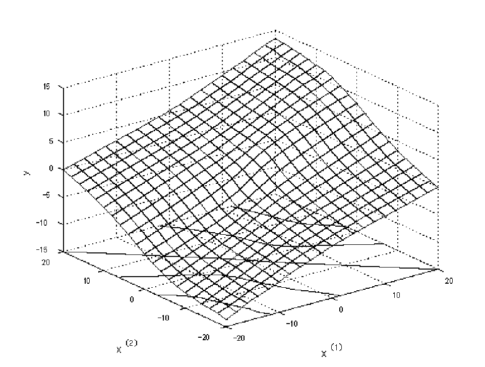
Next, we show an example of Bayesian prediction whose prior depends on the explanatory variables of future samples. We set x1=(3/2,1/2,0)⊤x_{1}=(\sqrt{3}/2,1/2,0)^{\top}, x2=(3/2,−1/2,0)⊤x_{2}=(\sqrt{3}/2,-1/2,0)^{\top}, x3=(0,0,1)⊤x_{3}=(0,0,1)^{\top}, y1=3/2+1/2y_{1}=\sqrt{3}/2+1/2, y2=3/2−1/2y_{2}=\sqrt{3}/2-1/2 and y3=0y_{3}=0. Figure 5 is a graph of EπS;A∗[y~|x~,y,x]E_{\pi_{S;A^{*}}}[\tilde{y}|\tilde{x},y,x] for each value of x~=(x~(1),x~(2),0)∈ℝ×ℝ×{0}\tilde{x}=(\tilde{x}^{(1)},\tilde{x}^{(2)},0)\in\mathbb{R}\times\mathbb{R}\times\{0\} with the rescaled Stein prior πΣ;A∗\pi_{\Sigma;A^{*}}. Here, the Bayesian estimation based on the uniform prior corresponds to the MLE β^=(1,1,0)\hat{\beta}=(1,1,0), i.e. y=x(1)+x(2)y=x^{(1)}+x^{(2)}.

Refer to caption
Figure 5: An example of Bayesian prediction whose prior depends on the explanatory variables of future samples.

We can see that the amount of shrinkage by the Bayesian prediction increases as the direction of x~\tilde{x} becomes closer to x(1)x^{(1)} than x(2)x^{(2)}, i.e. x~⊤​e1\tilde{x}^{\top}e_{1} becomes larger than x~⊤​e2\tilde{x}^{\top}e_{2}. This fact is intuitively explained as follows: when explanatory variables of training samples are closer to x(1)x^{(1)}, x~\tilde{x} whose direction is close to x(1)x^{(1)} has more information than ones whose direction is close to x(2)x^{(2)}. Thus x~\tilde{x} close to x(1)x^{(1)} need not be shrunk.

Figure 4 shows the risk functions of pIp_{I} and pΣp_{\Sigma} for d=3,5,7,9d=3,5,7,9 and ‖β‖∈[0,2]\|\beta\|\in[0,2]. The model has no intercept term. Here we assume that the columns of XX and X~\tilde{X} are independently sampled from N10​(0,I10)N_{10}(0,I_{10}).

Refer to caption
Figure 6: Comparison of the risk values by five predictive densities: the Bayesian predictive density based on pIp_{I} and pΣp_{\Sigma}, the ridge regression prior with regularization parameters λ=10\lambda=10 and λ=10=3.16\lambda=\sqrt{10}=3.16, and the plug-in density of the MLE. The model is five dimensional and has no intercept term. We generate 10410^{4} independent samples of XX and X~\tilde{X} from N10​(0,I10)N_{10}(0,I_{10}). Each line in the figure represents the sample mean of the risk RKL​(β,p^)R_{\rm KL}(\beta,\hat{p}) for the predictive density p^\hat{p}.

Figure 6 compares five predictive densities: the Bayesian predictive density based on pIp_{I} and pπΣp_{\pi_{\Sigma}}, the ridge regression prior with regularization parameters λ∈{10,10}\lambda\in\{\sqrt{10},10\}, and the plug-in density of MLE.

The ridge regression prior is

πR​R​(β,λ)=λd/2(2​π)d/2​exp⁡(−λ​‖β‖22)\pi_{RR}(\beta;\lambda)=\frac{\lambda^{d/2}}{(2\pi)^{d/2}}\exp\Big(-\lambda\frac{\|\beta\|^{2}}{2}\Big)

with a regularization parameter λ>0\lambda>0. We note that the posterior mean with the ridge regression prior is equivalent to the ridge regression estimator

β^R​R=(X​X⊤+λ​I)−1​X​y.\hat{\beta}_{RR}=(XX^{\top}+\lambda I)^{-1}Xy.

When ‖β‖\|\beta\| is close to 00, the center of shrinkage, the risk based on the ridge regression prior πR​R\pi_{RR} becomes smaller than that based on πΣ\pi_{\Sigma}. However, when ‖β‖\|\beta\| increases, the prediction with πR​R\pi_{RR} becomes worse than the one with πI\pi_{\rm I} and even worse than the plug-in distribution of the MLE.

6 Conclusions and discussions

In this paper, we considered the multivariate Normal model with an unknown mean and a known covariance. The covariance matrix can be changed after the first sampling. We assumed rotation invariant priors of the covariance matrix and the future covariance matrix. We showed that the shrinkage predictive density with the rescaled rotation invariant superharmonic priors is minimax under the Kullback-Leibler risk. Moreover, if the prior is not constant, Bayesian predicitive density based on the prior dominates the one with the uniform prior.

In this case, the rescaled priors are independent of the covariance matrix of future samples. Therefore, we can calculate the posterior distribution and the mean of the predictive distribution (i.e. the posterior mean and the Bayesian estimate for quadratic loss) based on some of the rescaled Stein priors without knowledge of future covariance. Since the predictive density with the uniform prior is minimax, the one with each rescaled Stein prior is also minimax.

Next we considered Bayesian predictions whose prior can depend on the future covariance. In this case, we proved that the Bayesian prediction based on a rescaled superharmonic prior dominates the one with the uniform prior without assuming the rotation invariance.

Applying these results to the prediction of response variables in the Normal regression model, we show that there exists the prior distribution such that the corresponding Bayesian predictive density dominates that based on the uniform prior. Since the prior distribution is independent of future explanatory variables, both the posterior distribution and the mean of the predictive distribution are independent of the future explanatory variables.

The robustness of some shrinkage methods as Stein estimators has been studied (see, for example, the bibliography in Robert 2001). The Stein effect has robustness in the sense that it depends on the loss function rather than the true distribution of the observations. Our result shows that the Stein effect has robustness with respect to the covariance of the true distribution of the future observations.

As the dimension of the model becomes large, the risk improvement by the shrinkage with the rescaled Stein prior πΣ\pi_{\Sigma} increases as in Figure 4. An important example of the high dimensional model is the kernel methods (see Hastie et al. 2001). As noted in Cristianini & Shawe-Taylor 2000, the feature space of kernel methods is a kernel reproducing Hilbert space whose dimension is as large as the sample size. Therefore Bayesian prediction based on shrinkage priors could be efficient for kernel methods. This is a future problem.

7 Acknowledgment

The authors appreciate Mr. Vu, Vincent Q. for precious comments on an earlier version of this paper.

Appendix A Finiteness of the marginal distribution

Here, we prove finiteness of the marginal distribution mπ​(μ,Σ)m_{\pi}(\mu,\Sigma).

Lemma A.1

If π\pi is a superharmonic prior density function, the marginal distribution mπ​(x,Σ)m_{\pi}(x,\Sigma) is finite for every vector x∈ℝdx\in\mathbb{R}^{d} and positive definite matrix Σ∈ℝd×d\Sigma\in\mathbb{R}^{d\times d}.

Proof. Fix a vector x∈ℝdx\in\mathbb{R}^{d} From the definition of superharmonic functions, π≢∞\pi\not\equiv\infty. Thus, ∃x0∈ℝd\exists x_{0}\in\mathbb{R}^{d} s.t. π⁡(x0)<∞\pi(x_{0})<\infty. If we set π~​(μ):=π⁡(μ+x0)\tilde{\pi}(\mu):=\pi(\mu+x_{0}), then π~\tilde{\pi} is superharmonic and π~​(0)<∞\tilde{\pi}(0)<\infty.

Let λmax\lambda_{\rm max} be the maximal eigenvalue of Σ\Sigma and r0:=‖x+x0‖r_{0}:=\|x+x_{0}\|, then

mπ​(x,Σ)\displaystyle m_{\pi}(x,\Sigma) ≤∫exp⁡(−‖x+x0−μ‖22​λmax)​π~​(μ)​𝑑μ\displaystyle\leq\int\exp\left(-\frac{\|x+x_{0}-\mu\|^{2}}{2\lambda_{\rm max}}\right)\tilde{\pi}(\mu)\mathrm{d}{\mu}
≤∫‖μ‖≤2​r0exp⁡(−‖x+x0−μ‖22​λmax)​π~​(μ)​𝑑μ+∫‖μ‖>2​r0exp⁡(−‖μ‖28​λmax)​π~​(μ)​𝑑μ\displaystyle\leq\int_{\|\mu\|\leq 2r_{0}}\exp\left(-\frac{\|x+x_{0}-\mu\|^{2}}{2\lambda_{\rm max}}\right)\tilde{\pi}(\mu)\mathrm{d}{\mu}+\int_{\|\mu\|>2r_{0}}\exp\left(-\frac{\|\mu\|^{2}}{8\lambda_{\rm max}}\right)\tilde{\pi}(\mu)\mathrm{d}{\mu} (26)

The first term of the right-hand side of (26) is finite because the integral of a superharmonic function over a compact subspace of ℝd\mathbb{R}^{d} is finite (see Theorem 4.10 of Helms 1969).

The second term is also finite because

∑n=2∞∫n​r0<‖μ‖≤(n+1)​r0exp⁡(−‖μ‖28​λmax)​π~​(μ)​𝑑μ≤C​∑n=2∞exp⁡(−(n​r0)28​λmax)​π~​(0)​{(n+1)​r0}d\sum_{n=2}^{\infty}\int_{nr_{0}<\|\mu\|\leq(n+1)r_{0}}\exp\left(-\frac{\|\mu\|^{2}}{8\lambda_{\rm max}}\right)\tilde{\pi}(\mu)\mathrm{d}\mu\leq C\sum_{n=2}^{\infty}\exp\left(-\frac{(nr_{0})^{2}}{8\lambda_{\rm max}}\right)\tilde{\pi}(0)\{(n+1)r_{0}\}^{d}

for a positive constant CC. Here we used a fact ∫‖μ‖<rπ~​(μ)​𝑑μ<C​π~​(0)​rd\int_{\|\mu\|<r}\tilde{\pi}(\mu)\mathrm{d}\mu<C\tilde{\pi}(0)r^{d} by Theorem 4.9 of Helms 1969. Therefore, mπ​(x,Σ)<∞m_{\pi}(x,\Sigma)<\infty. □\square

From this lemma, we see the assumption mπ​(z,v​Id)<∞m_{\pi}(z,vI_{d})<\infty in Theorem 2.4 (ii) is redundant.

References

  • Corcuera & Giummolé (2000) Corcuera, J. M. & Giummolé, F. (2000). First-order optimal prediction densities. In Applications of differential geometry to econometrics, P. Marriott & M. Salmon, eds. Cambridge: Cambridge University Press, pp. 214–229.
  • Cristianini & Shawe-Taylor (2000) Cristianini, N. & Shawe-Taylor, J. (2000). An Introduction to Support Vector Machines. Cambridge University Press.
  • George et al. (2006) George, E. I., Liang, F. & Xu, X. (2006). Improved minimax prediction under Kullback-Leibler loss. Annals of Statistics 34, 78–91.
  • Hastie et al. (2001) Hastie, T., Tibshirani, R. & Friedman, J. (2001). The elements of statistical learning – Data mining, inference, and prediction. springer series in statistics. New York: Springer.
  • Helms (1969) Helms, L. L. (1969). Introduction to Potential Theory. New York: Wiley-Interscience.
  • Komaki (1996) Komaki, F. (1996). On asymptotic properties of predictive distributions. Biometrika 83, 299–313.
  • Komaki (2001) Komaki, F. (2001). A shrinkage predictive distribution for multivariate Normal observables. Biometrika 88, 859–864.
  • Komaki (2006) Komaki, F. (2006). Shrinkage priors for bayesian prediction. Annals of Statistics 34, 808–819.
  • Lehmann & Casella (1998) Lehmann, E. L. & Casella, G. (1998). Theory of point estimation. New York: Springer, 2nd ed.
  • Liang & Barron (2004) Liang, F. & Barron, A. (2004). Exact minimax strategies for predictive density estimation, data compression, and model selection. Ieee Transactions on Information Theory 50, 2708–2726.
  • Murray (1977) Murray, G. D. (1977). A note on the estimation of probability density functions. Biometrika 64, 150–152.
  • Ng (1980) Ng, V. M. (1980). On the estimation of parametric density functions. Biometrika 67, 505–506.
  • Robert (2001) Robert, C. P. (2001). The Bayesian Choice. New York: Springer-Verlag, 2nd ed.